AutoDVS: An Automatic, General-Purpose, Dynamic Clock Scheduling System for Hand-Held Devices

(1)

AutoDVS: An Automatic, General-Purpose, Dynamic Clock

Scheduling System for Hand-Held Devices

Selim Gurun and Chandra Krintz

Computer Science Department

University of California Santa Barbara, CA

[email protected], [email protected]

ABSTRACT

We present AutoDVS, a dynamic voltage scaling (DVS) system for hand-held computers. Unlike extant DVS systems, AutoDVS dis-tinguishes common, course-grain, program behavior and couples forecasting techniques to make accurate predictions of future be-havior. AutoDVS uses these predictions in combination to guide dynamic voltage scaling. AutoDVS estimates periods of user inter-activity, user non-interactivity (think time), and computation per-program and system wide to ensure quality of service while reduc-ing energy consumption.

We describe our implementation of AutoDVS which consists of a set light-weight, Linux, kernel modules and user library routines for the iPAQ hand-held computer. We evaluate AutoDVS using real user workloads of iPAQ software that consist of interactive and soft-real time tasks executing alone and concurrently. Our re-sults indicate that AutoDVS decreases energy consumption signifi-cantly without negatively impacting user perception of system per-formance.

Categories and Subject Descriptors

D.4.8 [Operating Systems]: Performance—Modeling and

predic-tion, Measurements

General Terms

Measurement, Performance

Keywords

Voltage Scaling, Prediction, Power Consumption, Resource-constrained devices

1. INTRODUCTION

Recent advances in embedded device technology have led to the proliferation of battery-powered devices and, in particular, hand-held personal digital assistants (PDAs) and web-enabled cellular phones. Worldwide, approximately 30 million PDAs are in use, and predictions indicate that PDA sales in the US will increase from 6.9 million to 17.1 million by 2007 [16]. As a result of the popu-larity and improving capability of hand-held devices, users demand

Permission to make digital or hard copies of all or part of this work for personal or classroom use is granted without fee provided that copies are not made or distributed for profit or commercial advantage and that copies bear this notice and the full citation on the first page. To copy otherwise, to republish, to post on servers or to redistribute to lists, requires prior specific permission and/or a fee.

EMSOFT’05, September 19–22, 2005, Jersey City, New Jersey, USA.

increasingly complex software for these devices. Moreover, users expect lighter devices with long battery lives.

Dynamic voltage scaling (DVS) is a technique that can extend the battery life of hand-held devices without compromising system performance. DVS enables the CPU to be scaled dynamically ac-cording to varying workload demand. Using such functionality, a DVS system must determine the best clock speed for optimal per-formance and battery lifetime.

An important parameter in a DVS system is the frequency switch latency. While some CPUs, such as Transmeta Crusoe [22], are ca-pable of completing this operation with only millisecond delays, many lower-end systems, such as the ones we are targeting with this work, cannot. For example, for the popular, HP iPAQ H3800, we found that the frequency switch time is approximately 40 mil-liseconds. Unlike the previous DVS research [4, 3, 6, 7, 13, 21, 23], AutoDVS targets mobile systems where user interactive per-formance is crucial and a frequency switch is costly.

AutoDVS couples multiple behavior-detection policies into a sin-gle system to identify accurately periods of user interactivity as well as high and low CPU demand. The user interactivity policy maintains the expected load and length of user activity period for each active GUI application. To compute these parameters, Au-toDVS employs NWSLite [8], a time-series based prediction tool that we developed in prior work.

For non-interactive periods, AutoDVS employs two interval sched-uling techniques. AutoDVS implements variations of PAST work-load prediction [23] and Pering’s hysteresis [18] to capture CPU in-tensive periods in the workload and to scale the CPU appropriately. AutoDVS also monitors Linux idle process statistics to identify op-portunities to scale-down the CPU.

Our experimental results indicate that AutoDVS can reduce power consumption significantly without degrading system performance. We empirically evaluate AutoDVS for real iPAQ workloads that we collected from actual users. For repeatability, we play-back the workloads in real time on the iPAQ, and measure the impact of us-ing AutoDVS and comparative approaches. On average, AutoDVS reduces power consumption by 49% for interactive tasks and by 31% for concurrent workloads.

In the following section, we present some background on dy-namic voltage scaling and on existing approaches to DVS that we incorporate into AutoDVS. We then describe the design and imple-mentation of AutoDVS in Section 3. In Section 4, we present the empirical evaluation of our system and in Section 5, we conclude.

2. BACKGROUND

In modern, embedded-device, CPUs, most energy is dissipated in the form of dynamic power consumption [20, 15]. Dynamic power is a function of CPU voltage and frequency and is approximated

(2)

by:

P∝V2f (1)

When scaling the voltage, we must scale the frequency in the same proportion to meet signal propagation delay requirements [19]. By decreasing the voltage, we have the potential for quadratic power savings with a possible linear performance loss.

To minimize the effect of voltage scaling on system responsive-ness, DVS policies must estimate future workload and choose the most appropriate CPU level. Accurately predicting future workload is challenging yet vital for maintaining acceptable performance. Mis-prediction can result in setting the CPU level too high, curtail-ing power savcurtail-ings, or in settcurtail-ing the CPU level too low, produccurtail-ing an unresponsive system.

The goal of our work is to develop an effective DVS system for iPAQ hand-helds and their applications. The result is a system called AutoDVS that is an adaptive runtime technique that effec-tively reduces power consumption in a way that is transparent to the device user. AutoDVS is general-purpose (unlike other DVS-enabled operating systems such as GraceOS [26] for multimedia devices), and fully automatic, i.e., it requires no application sup-port or programmer effort (as is required in DVS systems such as Chameleon [11]). To implement AutoDVS, we have incorporated and extended existing DVS techniques for interval scheduling and interactive task scheduling.

Interval Scheduling

Interval schedulers [23, 7, 6, 21] divide the workload into fixed-length time intervals. These techniques use measurement history to estimate the workload in a future interval. For example, the PAST interval scheduler [23] assumes that the load in the next interval will be same as that in the last interval; theAV GNinterval

sched-uler [23, 7] assumes that the next interval is an exponential moving average (using a decay factor) of the N previous intervals. Other interval schedulers use observation heuristics [6] and more sophis-ticated statistical estimation methods [21] to estimate workload.

The efficacy of interval scheduling however, has proven to be limited in practice. Extant approaches use fixed-length, short inter-vals, i.e., 1-50ms, to accommodate for responsiveness requirements of interactive applications. However, for most applications the uti-lization pattern is visible only when deploying functions that span a larger period. For example, for an MPEG application, this pattern may not be visible even with a one second moving average [7].

Another limitation of prior approaches to interval scheduling is that they assume very short voltage switch latency (on the order of hundreds of microseconds) [7, 3]. Even though it is possible to achieve this rate on very specialized CPUs, e.g., the Transmeta Cru-soe, most handheld devices such as the HP iPAQ use much simpler hardware. Moreover the operating system must alert all synchro-nized peripheral devices that CPU speed is changing. These imple-mentations can significantly increase the time required to complete a switch between frequency levels.

Interactive Task Scheduling

Recent DVS studies have focused on classifying tasks into different groups, each with a customized policy. [4] suggests three groups: Interactive, periodic, and background tasks. For interactive tasks, the system computes the optimum performance factor (OPF). The OPF is the fraction of CPU speed required to complete a task no later than the user perception threshold. [4] defines this threshold as 50 milliseconds. The system in this prior work estimates the CPU load for a particular task in an interactive episode using an average of past CPU demand of the task, weighted by episode duration.

A periodic task consists of a producer-consumer pair. The sys-tem schedules a periodic task using an estimate of the time period between the completion of a producer and the start of a consumer. The system computes CPU speed such that producer ends immedi-ately prior to when the consumer starts; the system uses the same CPU speed for both the producer and consumer.

Vertigo [3] is a refined and simplified implementation of this ap-proach. Instead of categorizing tasks as producer and consumer, Vertigo maintains individual CPU utilization statistics for each task. Vertigo recomputes CPU utilization each time it attempts to resched-ule a task. To identify interactive tasks, Vertigo monitors GUI events. When an event arrives, Vertigo marks the window man-ager and the recipient of GUI event as interactive. If any task com-municates with an interactive task, Vertigo marks it also as inter-active. The interactive period continues until all marked tasks are pre-empted by other tasks. Marking can be quite complex to im-plement, as tasks can use a variety of methods to communicate. Unfortunately, the implementation details and source code of Ver-tigo are not publicly available.

Lorch et al. suggest an approach that specifically targets user in-teractivity [13]. The system labels a user event with the type of GUI event that initiates it, e.g., a key-press, mouse-click, or drag event. Each event type has a separate DVS policy. The authors of this approach compute the CPU schedule using PACE [12]. PACE is a heuristic that the authors have proven to be optimal for computing CPU speed when (a) CPU can change frequency on a continuous scale, (b) all task deadlines are known, and (c) the cumulative dis-tribution function (CDF) of task CPU demand is known.

All approaches that target user interactivity must overcome the challenge of determining when a task will complete without assis-tance from the application. The approach in [4] requires task com-pletion time to update task execution time; the approach in [13] uses task completion time to compute task CDF and deadline. The former solution is precise, but is inherently complex; it requires monitoring system calls and communication between threads. The latter solution suggests an event is complete if a new event is posted or the idle thread is running and no I/O is ongoing. Even though this second approach can occasionally mis-classify a task as com-plete, it is more attractive due to its simplicity. In the next section, we articulate how we couple and extend these prior techniques for interval and interactive task scheduling to overcome the challenges and limitations, and yet to achieve the benefits, of each.

3. AUTODVS

Our goal with AutoDVS is a light-weight, practical DVS system for low-end, mobile computers and their applications – without par-ticipation from the user, information from the source programs, or a priori knowledge of task length or behavior. AutoDVS transpar-ently changes the clock frequency according to the workload activ-ity that it senses dynamically. The key to the efficacy of AutoDVS is its categorization of application workload into two session types: interactive sessions and batch sessions. AutoDVS then intelligently applies different, independent, and multiple scheduling policies to each session type.

For interactive sessions, AutoDVS employs a user-space policy that considers GUI events for each application. The policy predicts the duration and CPU load of each interactive session. By consid-ering each application individually, our predictions have a better chance of capturing regular, repeating patterns within each.

For batch sessions, AutoDVS implements two different kernel-level, interval-based policies (as Linux kernel modules). The batch policies identify changes in CPU load and estimate when a CPU clock change is warranted. These CPU load predictors take a global

(3)

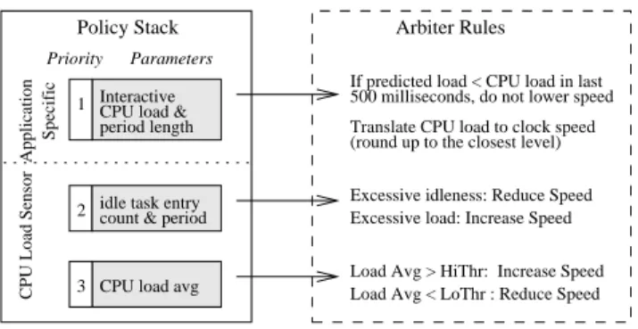
CPU load avg count & period idle task entry 2

3

Arbiter Rules Policy Stack

Excessive idleness: Reduce Speed

Load Avg > HiThr: Increase Speed period length

CPU load & Interactive 1

Application

Specific

Priority Parameters

CPU Load Sensor

Excessive load: Increase Speed

Load Avg < LoThr : Reduce Speed Translate CPU load to clock speed (round up to the closest level) 500 milliseconds, do not lower speed If predicted load < CPU load in last

Figure 1: AutoDVS policy stack and arbiter rules. AutoDVS responds to policy requests according to priority (1 is highest).

view of the system to identify additional DVS opportunities not made apparent by the fine-grain interactive scheduler.

All CPU performance change requests issued by any policy are handled by an arbiter using the pre-defined rules that we show in Figure 1. The policies either request a speed change or inform the arbiter about expected CPU load and load duration. The arbiter exe-cutes requests using a priority scheme; the requests from interactive applications have the highest priority, and the requests from poli-cies that monitor largest time-span have the lowest priory. In the case of concurrent requests, the arbiter always chooses the highest priority. However, there is one exception to this rule: If the pol-icy that monitors excessive load detects a sudden increase in CPU demand, this request is honored first.

This division of labor across the system is key to the efficacy of AutoDVS. Together the policies are able to consider a wide range of application behaviors without much implementation complex-ity. By processing the requests centrally, we are able to make accu-rate and effective, system-wide, CPU scaling decisions that reduce power consumption without negatively impacting performance.

Moreover, this design accounts for the actual CPU change la-tency of the underlying device. Extant approaches to DVS schedul-ing assume a very low latency and allow a large number of fre-quency changes. For real devices however, as we suggested previ-ously, this latency can be much larger due to the overhead of main-taining other devices in the system that are synchronized with the CPU clock. We measured the switch overhead for the HP IPAQ H3800 running Linux 2.4 to be 40 milliseconds on average.

Figure 2 shows the timeline of a clock speed change request on this platform. We measured this period using timestamp counters. Initially, the kernel maintains a dynamic list of device drivers that must be alerted when the clock speed changes. A frequency switch request requires three traversals of this list; first to inquire if new speed is in acceptable range, and then to let device drivers initial-ize their hardware appropriately before and after clock change, i.e. PRECLK and POSTCLK phases. During the PRECLK and POST-CLK phases, the device drivers impose initialization delays due to hardware requirements. Even though these delays do not block the CPU, they increase the latency between clock speed request and ac-tual change. The more devices that employ the CPU clock for tim-ings, the longer this latency. AutoDVS does not consider sessions shorter than 50 milliseconds to account for this latency. Moreover, we can change this threshold dynamically to adapt to changing pe-ripheral configurations. milliseconds 40 0 POSTCLK 35 PRECLK Phase Clock Scheduling Rqst

old speed new speed

time

Update Clock Speed

Figure 2: iPAQ H3800 clock scaling request timing. After re-ceiving the request, the kernel initializes data structures and waits for initialization of hardware devices (PRECLK and POSTCLK phases). The actual clock scheduling takes under a millisecond (heavily shaded area). The clock scheduling latency on iPAQ Linux Kernel v2.4 is approximately 40 milliseconds.

3.1 Interactive Tasks

AutoDVS monitors GUI events to identify interactive sessions in arbitrary programs. Our system employs no notion of tasks, but instead automatically infers task-like behavior, i.e., periods of time, in which the user is interacting with the device. We refer to non-interactive sessions as think times. In addition, we do not distin-guish event types (as is done in [13]) i.e, we consider only inter-active sessions regardless of which events occur within them. The goal of AutoDVS is to predict the length of user interactivity and and utilization level, which is crucial to prevent obtrusive effects of frequent clock scaling requests.

3.1.1 Monitoring GUI Events

For each application, AutoDVS monitors user input and display updates. The former events are the direct result of user input through the keypad and touch-screen. The latter events include GUI mes-sages such as window update and focus operations. Monitoring the display updates is important to correctly identify interactivity, e.g., when user waiting for an application to redraw the screen.

In our software platform, all GUI applications are linked against a shared GUI library. We extended theevent handlerfunction of this library to contain AutoDVS policies. Theevent handler is a null (unimplemented) wrapper that receives all GUI events be-fore any other function. Our modifiedevent filteridentifies interactive sessions and interfaces to the prediction library to fore-cast interactive session lengths and load (we detail this process in the next subsection). We implemented a Linux new system call to provide a communication path to AutoDVS policies in the kernel.

3.1.2 DVS for Interactive Sessions

An interactive session starts with the arrival of an event and ends if no event is received for a period oftp. Identifying the interactive

sessions correctly is important, since presumably, the user is most sensitive to any performance loss during these periods. The value oftpimpacts the system in two ways. Iftpis too small, the

algo-rithm might end an interactive session prematurely while the appli-cation is still processing a GUI event. Iftpis too large, AutoDVS

will maintain a high CPU speed and miss opportunities for reduc-ing energy consumption. We settpto be 1 second empirically: our

evaluation of more than110,000events on iPAQ workloads indi-cates that the inter-arrival time between two GUI events is less than 1 second more than 99.0% of time and that when inter-arrival time is larger than 1 second, the mean time to receive next event is 8 seconds.

When an interactive session starts, AutoDVS computes two pa-rameters: the length of the previous session and the interactive CPU load. The computation of length (tp) is straightforward. Ifeiis the

(4)

arrival time of an event such that the period betweeneiand

preced-ing event is larger thantp. Then the length of periodiis equal to

(ei+1−e_i). We set the CPU load to be the CPU time divided by

length of the period. To predict the new session length and CPU load, we employ NWSLite [8].

NWSLite is a time-series-based prediction utility for embedded devices that we developed in prior work. It is an extension of the Network Weather Service [24] for Computational Grid Comput-ing [5]. NWSLite performs non-parametric statistical forecastComput-ing using a mixtuof-experts approach for prediction rather than re-lying on a single model, i.e., it implements a set of time-series mod-els, each having its own parameterization. Internally, the predictor for each model generates a forecast. NWSLite ranks predictors by computing the cumulative prediction errors and chooses the predic-tor with the highest rank for the next prediction. The CPU require-ments of NWSLite is low – it uses 55 floating operations and 592 integer and miscellaneous operations per forecast. The memory de-mand of NWSLite is also minimal as its forecasters do not require prediction history.

3.2 CPU Load Sensor

AutoDVS must also account for periods of time during workload execution that are not interactive. Most programs, even those that are primarily interactive, execute think (non-interactive or compu-tationally intensive) periods. The CPU load sensor is responsible for these sessions. This sensor takes a global view of the system and workload, i.e., it does not consider task-level and application-specific details. CPU load sensor employs two interval-schedulers:

CPU Load Monitor and the Idle Process Monitor.

The CPU load monitor considers very large intervals (10 sec-onds) and averages the measured CPU load across intervals. By averaging, the monitor eliminates noise in the data and distributes

slack time more efficiently. Slack time consists of the idle cycles

during an interval when CPU utilization is less than 1. The monitor predicts that the CPU load for the next interval will be the same as it is for the current interval (this is the PAST policy used in [23, 7]). We do not use NWSLite for predicting future load since it requires floating point operations which cannot be handled in the Linux ker-nel. By coupling interactive task scheduling with the CPU load monitor, AutoDVS can handle both fine and coarse grain workload activities. However, we require one additional monitor to identify fine-grain behavior in non-interactive (e.g. batch and background) sessions, called the idle process monitor.

The idle process is a process that the OS scheduler executes whenever no other process in the system is runnable. The idle pro-cess monitor evaluates (then resets) idle propro-cess statistics every 500 milliseconds. The monitor considers the number of times the idle process was scheduled by the OS and its execution duration during the previous interval. We modified the Linux scheduler (sched.c) to collect and export this information as a kernel symbol. All of our modifications are light-weight, simple, and efficient and do not perceivably impact the behavior of the system.

Both monitors make CPU scaling requests to the arbitrator. The CPU load monitor uses an extension to Pering’s hysteresis pair [18] to decide when to request a speed change. These values, (50,70) in prior work, act as a boundary for average CPU load. A level less than 50% indicates CPU can be scaled down and a level higher than 70% indicates CPU can be scaled up. We found empirically that the pair (60,80) works best in our actual implementation for iPAQ software. The idle process monitor requests a step increase from the arbitrator when it detects a period (500 milliseconds) in which the idle process is never scheduled. If the monitor detects that the idle process executes for over half the interval time, it requests a

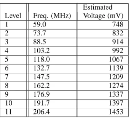
Estimated Level Freq. (MHz) Voltage (mV)

1 59.0 748 2 73.7 832 3 88.5 914 4 103.2 992 5 118.0 1067 6 132.7 1139 7 147.5 1209 8 162.2 1274 9 176.9 1337 10 191.7 1397 11 206.4 1453

Table 1: SA1100 Parameters. We estimate the voltage levels using equations 2 and 3, and assuming that the SA1100 has the same characteristics as the XScale processor.

step decrease.

Both monitors request only single step CPU clock changes.We investigated methods such as estimating CPU cycles based on work-load demand and directly switching to the most appropriate clock level (i.e. similar to [4]), however, these approaches resulted in instability, i.e. the system switched back and forth rapidly between neighboring frequency levels. The reason for this thrashing is a combination of measuring the CPU during periods of fluctuation (which impacts the measurement process) and hardware design [7].

4. EVALUATION

We have empirically evaluated the efficacy of our approach by running a large number of very different workloads on an iPAQ with AutoDVS and comparative techniques. In the subsections that follow, we describe our experimental setup and the benchmark workloads. We then define the metrics that we use in our empirical evaluation and present our results.

4.1 Experimental Platform

Our device infrastructure includes five Compaq H3800 hand-held computers running Familiar Linux version 0.7.2 [2]. The H3800 is a very typical hand-held computer, with a 206MHz StrongArm CPU, and 64 Mbytes of main memory. It is capable of dynamic frequency scaling, however, it does not yet support voltage scaling. To estimate power savings due to voltage scaling, we use a tech-nique defined in prior work [4] for a similar study. We assume that the StrongArm and XScale [10] processor exhibit similar power characteristics and use published data for the XScale XSA (the sys-tem most similar to the StrongArm in terms of maximum voltage and supported frequency range), in the estimation. We approximate the voltage levels of the XScale CPU using the available frequency levels and a second degree polynomial parameterized by the XSA data:

v=−4×10−7f2+ 0.0015f+ 0.5324 (2)

To compute the corresponding StrongArm voltage levels, we use Equation 3 as a mapping function. That is, we linearly scale the StrongArm frequency range to the XScale frequency range:

f0₌ 773−150.0

206.4−59.0

×(f−59.0) + 150.0 (3)

We present the estimated voltage levels in Table 1.

The StrongArm architecture requires that all of the primary pe-ripherals be synchronous to the CPU clock [9]. This implies that all

(5)

Event Count

Trace (ETime@206MHz) Description

DrawPad-1 23100 (915.4s) Drawing random pictures General use including calendar, General-1 3688 (448.1s) contacts and games

Solitaire-1 8700 (756.4s) Multiple Solitaire games Tetrix-1 6936 (583.8s) Tetrix

Tetrix-2 1342 (210.1s) Tetrix - very short and slow Checkers-1 1238 (205.1s) Checkers - medium difficulty Checkers-2 1214 (265.7s) Checkers - maximum difficulty Checkers-3 2490 (1076.4s) Checkers - maximum difficulty

Table 2: Event traces that we use in our results. We gather the traces using instrumented versions of the system while different users exercised the iPAQs. We name each trace to reflect the application that was dominant during the usage period.

CPU scaling will impact the performance of memory, the I/O con-troller, DMA, the LCD concon-troller, etc. The dependency between the CPU clock and external devices can cause significant differ-ences between theoretical expectations (and simulated results) and practical results. For example, Grunwald et al. found that the CPU utilization changes non-linearly with respect to clock frequency, possibly due to variations in memory access cycles [7]. Another obstacle was the LCD driver. In our evaluations, the display started vibrating making it unreadable for any speed lower than 103MHz. Thus we had to eliminate three lowest frequencies.

The window manager that we run on the devices is Opie [17] version 1.0.2. Opie is an open-source graphical user interface de-signed for Sharp Zaurus and Compaq hand-held computers. It is a full-fledged GUI comparable to commercial versions in both ap-pearance and features. The available Opie applications include Cal-endar, Contacts, Drawpad, a multimedia player, a wide range of games, etc.

4.2 Benchmarks and

Experimental Methodology

We evaluate AutoDVS below using two different scenarios. (1) Interactive: Running GUI applications; and (2) Concurrent: Inter-active and soft-real time applications running together.

To evaluate and compare the performance of interactive appli-cations, we collect a set of usage traces and extracted event and timestamp information. We then monitor the performance of Au-toDVS while replaying the events in real time. Thus, our results

also include the overhead of clock switching and all AutoDVS func-tionality.

To collect the usage traces, we have installed Opie on several Compaq H3800 hand-held computers and have distributed them to graduate students in our department. We alert the students that we are capturing all events and ask them to use the hand-helds as their own as normally as possible and to reboot them periodically (to end the session).

We modify the iPAQ software to enable trace collection in three ways: We (1) disable network connectivity; (2) modify random number generators to use a fixed seed; and (3) program each to clear all user state information after every reboot. These changes were necessary to eliminate as much non-determinism as possible so that we could re-generate the user events in the correct order during experimentation.

To capture the events, we instrument the Linux kernel at the I/O driver level. Our system captures all events generated by the touch-screen, the keypad, and the joy-pad using a microsecond times-tamp. We save the identification information for captured events in

RAM and copies them to permanent storage immediately prior to shut-down, to prevent any excessive overhead. The time and space overhead for event trace collection is small. Each event requires a total of 20 bytes: 8 bytes for the timestamp and 12 bytes for event type and attributes. Since we capture events at the I/O device driver, we can read the current time directly from Linux kernel data structures and no system calls are required.

To replay the captured events, we have developed a Linux kernel module. The module initiates events from a list in memory using a microsecond resolution timer.

The events describe user behavior from boot-up to shutdown. Some of the event traces that we captured are not useful; they are either too short, broken, i.e., dependent on user created files, or too similar. Overall, we employ the traces described in Table 2. The second column is the number of events in the trace and the total time (seconds) for the real time play-back at maximum per-formance (206MHz). We refer to each event trace using the name of the application that was active most often. The first four traces describe more general-use applications and include multiple pro-gram types. The last four traces are exclusively games.

To evaluate soft real-time applications we use Madplay, an open-source, high quality, MP3 decoder [14]. We interface Madplay to the GNOME Enlightened Sound Daemon (ESD), to enable on-line playback. The input file encoding rate is 56Kbits/sec.

4.3 Evaluation Metrics

We have evaluated the impact of AutoDVS using three different metrics: energy factor, stall rate, and stall magnitude. Energy fac-tor measures energy consumption with respect to execution at full CPU performance. The stall rate and magnitude metrics describe the degradation in interactive performance due to CPU scaling.

We compute energy consumption using theenergy factor

(EF) as defined in [4].EFis the ratio of energy used by the scaled workload to energy used when workload is processed at full speed. That is, EF= Pn i=1v 2 ifiti v2 M AXfM AXT (4) wherevi andfiare the voltage and frequency of each period of

time (ti) between two frequency scaling operations andT is the

execution time of benchmark at full CPU performance level. We use the frequency and voltage levels that are given in Table 1.EF

is unit-less and measures the energy consumption of the CPU only. To compute performance loss, we record the execution time of each interactive event. Specifically, we assume that execution of an event starts when it arrives at the window manager. We define event completion time using the approach described in [13]: The execution of an event ends when the idle task is entered and no I/O is ongoing. Even though this method can be imprecise (i.e. it might occasionally mis-classify events as completed), other (ex-tant) approaches (described in Section 2) are highly complex and can adversely affect the performance of monitored system. We dis-cuss the impact of using this method when we present our results.

We assume that an event misses its deadline if its execution time is larger than user perception threshold, i.e. 50 milliseconds [4]. Given thatdis the deadline, andmkis the execution time of an

event which missed its deadline, the stall rate (SR) is:

SR=

Pn

k=1(mk−d)

T (5)

SRis a unit-less metric that measures the user perceived perfor-mance loss during the execution of a benchmark. However this metric does not indicate how much the user must wait for a stalled

(6)

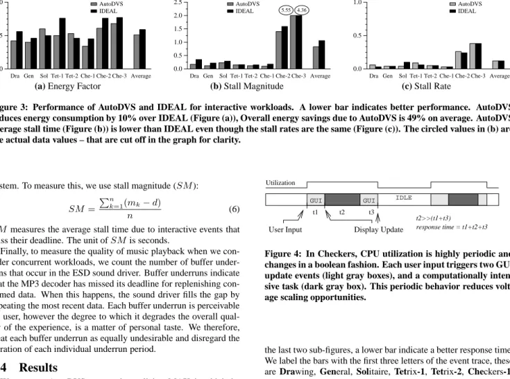
Dra Gen Sol Tet-1 Tet-2 Che-1 Che-2 Che-3 Average

0.0 0.5

1.0 AutoDVS IDEAL

0.0 0.5 1.0 1.5 2.0 2.5 AutoDVS IDEAL 5.55 4.36

0.0 0.5

1.0 AutoDVS IDEAL

(a) Energy Factor (b) Stall Magnitude (c) Stall Rate

Figure 3: Performance of AutoDVS and IDEAL for interactive workloads. A lower bar indicates better performance. AutoDVS reduces energy consumption by 10% over IDEAL (Figure (a)), Overall energy savings due to AutoDVS is 49% on average. AutoDVS average stall time (Figure (b)) is lower than IDEAL even though the stall rates are the same (Figure (c)). The circled values in (b) are the actual data values – that are cut off in the graph for clarity.

system. To measure this, we use stall magnitude (SM):

SM=

Pn

k=1(mk−d)

n (6)

SMmeasures the average stall time due to interactive events that miss their deadline. The unit ofSMis seconds.

Finally, to measure the quality of music playback when we con-sider concurrent workloads, we count the number of buffer under-runs that occur in the ESD sound driver. Buffer underunder-runs indicate that the MP3 decoder has missed its deadline for replenishing con-sumed data. When this happens, the sound driver fills the gap by repeating the most recent data. Each buffer underrun is perceivable by user, however the degree to which it degrades the overall qual-ity of the experience, is a matter of personal taste. We therefore, treat each buffer underrun as equally undesirable and disregard the duration of each individual underrun period.

4.4 Results

We compare AutoDVS to two other policies: MAX, in which the CPU is set to the highest level (for maximum performance), and IDEAL, in which we employ an ideal (oracle-based) CPU speed. IDEAL is not a realistic policy; it always chooses a clock speed such that its performance degradation is at the level of AutoDVS or less. To accomplish this, IDEAL uses future information: If IDEAL is worse than AUTODVS in terms of both performance metrics (i.e: SRand SM), or if the quality of sound playback is inadequate (i.e. more than 10 buffer underruns), then IDEAL switches to a higher clock frequency. We limited IDEAL choices to 132MHz, 176MHz and 206MHz to limit the search space.

We have experimented with two different scenarios. (1) Inter-active: Running GUI applications; and (2) Concurrent: Interactive and soft-real time applications running together. We describe the results from each of these scenarios in the following subsections.

4.4.1 Interactive Workloads

We first evaluate AutoDVS in terms of performance degradation during the execution of interactive applications. The IDEAL pol-icy has an advantage in this dataset; our empirical evaluations show that most interactive tasks require only a fraction of the maximum CPU power. A flat policy of 132MHz will provide adequate per-formance. The question we want to answer is this: Can AutoDVS achieve similar energy savings and still maintain a high level of responsiveness?

Figure 3 compares AutoDVS and IDEAL in terms of energy fac-tor, stall magnitude, and stall rate, from left to right. For all sub-figures, a lower bar indicates a better performance. For the first sub-figure, a lower bar indicates reduced energy consumption, for

IDLE GUI GUI Display Update Utilization User Input t3 t1 t2 response time = t1+t2+t3 t2>>(t1+t3)

Figure 4: In Checkers, CPU utilization is highly periodic and changes in a boolean fashion. Each user input triggers two GUI update events (light gray boxes), and a computationally inten-sive task (dark gray box). This periodic behavior reduces volt-age scaling opportunities.

the last two sub-figures, a lower bar indicate a better response time. We label the bars with the first three letters of the event trace, these are Drawing, General, Solitaire, Tetrix-1, Tetrix-2, Checkers-1, Checkers-2 and Checkers-3, from left to right. For example, for the Drawing benchmark, the AutoDVS policy saved almost 60% of energy with a 10% stall rate and approximately 240 milliseconds stall magnitude (i.e. mean stall time due to interactive events that miss their deadline).

We omit data from the MAX policy due to space constraints, however, we use MAX to explain some of the anomalies. In gen-eral, MAX policy always outperforms the other policies in terms of performance and always uses the most amount of energy.

AutoDVS enables significant performance benefits for the first six benchmarks. While keeping the stall rate under 10% of to-tal execution time, AutoDVS reduces energy consumption 30–66% (49% on average). In general, energy consumption is proportional to the performance requirements of benchmarks. For example, for Gen-1 and Che-1, which both include game sessions at novice levels, the savings are the greatest. For the first six benchmarks, IDEAL uses 176MHz for Tet-1 only and 132MHz for the rest. In general, IDEAL uses almost 10% more energy to maintain the stall rate of AutoDVS. However, AutoDVS is able to predict CPU demand accurately to reduce stall time. On average, AutoDVS achieves a 35% improvement over IDEAL.

Che-2 and Che-3 exhibit different behavior patterns than the other benchmarks. Both of these traces are game sessions at the highest difficulty level. As Figure 4 shows, their workload is very regular and highly computationally intensive. Each user input triggers a computationally intensive task which is followed by a long idle pe-riod (think time). The NWSLite is unable to predict this behavior accurately. It is possible to estimate such behavior using techniques such as spectral analysis [1], however, we avoid such algorithms in

(7)

0.0 0.5

1.0 AutoDVS

IDEAL

0.0 0.5 1.0 1.5 2.0 2.5 AutoDVS IDEAL 2.92 2.98

0.0 0.5

1.0 AutoDVS IDEAL

(a) Energy Factor (b) Stall Magnitude (c) Stall Rate

Figure 5: Performance of AutoDVS for interactive and soft-real time workloads running concurrently. A lower bar indicates better performance. The overall energy savings is 31% for AutoDVS and 20% for IDEAL (Figure (a)). Figures (b) and (c) report stall magnitude and rate, respectively. The circled values in (b) are the actual data values – that are cut off in the graph for clarity.

NWSLite due to their high computational (floating point) cost. De-spite some prediction error, AutoDVS enables energy consumption for Che-2 and Che-3 that is 36% lower than MAX and 15% lower than IDEAL.

4.4.2 Concurrent Workloads

We next investigate how AutoDVS performs when multiple ap-plications are running concurrently on an iPAQ. In particular, we replay the event trace while running the Madplay MP3 decoder (music player) in the background. For each event trace, we start collecting the measurement statistics when the two tasks begin ex-ecuting events concurrently; we continue measuring until Madplay terminates. There are three short-traces that end earlier than Mad-play, Tet-2, Che-1 and Che-2. For these traces, Madplay is the single task for 45%, 42% and 33% of total evaluation time, respec-tively. The Madplay playback length is 424 seconds.

The opportunities for CPU scaling are reduced when we exe-cute multiple programs concurrently. The question that we are in-terested in is whether it is possible to extract any energy savings without hurting performance.

Figure 5 compares the performance of AutoDVS to IDEAL using the same methodology as the previous subsection. AutoDVS is able to save 31% of the energy consumption over MAX on average. The energy savings of IDEAL is 20%. IDEAL chooses 176MHz for all but Che-2 and Che-3. For these two traces, IDEAL uses the maximum level (206MHz). The savings are small for traces with high computational requirements, e.g., Che-3 and Sol.

At the 132MHz (lowest) level, the buffer underruns for Mad-play are very high (122–2781) for all benchmarks. At 176MHz, there are fewer than 3 underruns. However, IDEAL must switch to 206MHz (the highest level) for Che-2 and Che-3 to achieve the same performance as AutoDVS. For example, Che-2 at 176MHz imposes a 8% larger stall rate and an average stall time that is 179 milliseconds worse than AutoDVS. The performance loss margin is greater for Che-3. The buffer underrun count is always less than 3 for AutoDVS. For MAX, buffer underruns are always 0.

In the concurrent workload results, the only anomalous case in which IDEAL outperforms AutoDVS in terms of energy consump-tion is for Solitaire. AutoDVS uses 13% more energy than its competitor to achieve approximately same performance level. Soli-taire is unique in that most of the GUI events are mouse drag/drop events; the other benchmarks use keypad, joypad, or touchscreen keyboard for most of the data input. Each drag and drop generates a sudden burst of GUI events (i.e. window update messages and mouse movements). Consequently, this sudden burst is accompa-nied with a jump in CPU demand. NWSLite immediately chooses the most aggressive forecaster, often over-estimating the CPU load for the next interactive session. Even though the CPU load sensor policies correct the over-estimation afterwards, some portion of

en-Parameter Value Description D 50 Msecs Task deadline

WC 6.192 Mcycles Worst-case execution cycles r 6 Number of transition points f (103.2 - 206.4) MHz StrongArm Clock frequency s [WC-1] / r Transition period -evenly spaced

0.05 Trim error parameter

Table 3: Simulation parameters that we used to investigate the efficacy of integrating PPACE into AutoDVS.

ergy is wasted during this period. Moreover, an increase in clock speed does not reduce the stall magnitude significantly since it is already very low.

We can address this problem in two ways:(1) by classifying drag and drop events separately from other GUI events and reducing the weight of events generated in bursts, or by (2) shutting down predictors that consistently over-estimate. We will evaluate these solutions in future work.

4.4.3 Integrating PACE

As a final experiment, we investigate the efficacy of extending AutoDVS to conserve additional energy on platforms that have very low voltage switch latency. To investigate this, we have incorpo-rated extant, efficient, implementation of the PACE algorithm [12, 13], called Practical Pace (PPACE) [25], into AutoDVS.

PACE is a technique that computes optimal energy savings when

continuous CPU scaling is possible. PACE computes CPU speed

as a function of completed work and gradually increases the CPU frequency as the task nears its deadline. PPACE extends PACE to handle discrete CPU scaling levels and uses a polynomial time approximation of PACE that is computationally efficient but does not always find the optimal solution.

We investigate the impact of integrating PPACE into AutoDVS. We employ simulation for these experiments (unlike in our previ-ous experiments) since an actual, online implementation of PPACE is currently not feasible due to three primary reasons. First, extent hand-held devices impose a very high switch latency. Second, the computational requirements of PPACE are high and consume sig-nificant resources in modern devices. Third, the computation of cumulative distribution function requires off-line information.

Despite these limitations, we are interested in understanding the potential of coupling PPACE and AutoDVS for interactive pro-grams. For these experiments, we consider the energy consumption

due to GUI events alone. Our results indicate the potential energy

savings during the execution of pre-deadline cycles. By definition, the PACE algorithms do not reschedule post-deadline cycles.

(8)

0.0 0.5 1.0

Figure 6: Simulated energy savings ratio with respect to Au-toDVS when we integrate PPACE. These results are different from all those prior in that we obtain them through simulation and consider only GUI events. Higher bars are better. On aver-age, incorporating PPACE results in a potential 41% decrease in energy consumption of GUI events when the event deadlines and WCETs are known a priori.

an additional API through which it consumes off-line information, task deadlines, and the worst-case execution times (WCETs) of tasks from the program. Table 3 shows the parameters we use to evaluate PPACE in AutoDVS. To determine the WCET in cycles, we use the CPU demand of 99 percentile of GUI tasks which is equal to 6.192 Mcycles. We limited the number of clock speed transitions to 6, placing them evenly in the range [1,WCET]. Even though we use a smaller number of transitions than were used in the previous PPACE, our implementation provides a higher resolu-tion than the original implementaresolu-tion since we use a much smaller

WCET. Xu et al. usesW C = 500Mcycles with100transition

points – this corresponds to a transition point approximately every 5Mcycles. In contrast, we place a transition point at approximately every1Mcycles.

Figure 6 shows the energy savings ratio for GUI events when we reschedule CPU speed using PPACE – relative to AutoDVS (not MAX as in prior graphs). Higher bars are better. The data indicates that using PPACE with AutoDVS can potentially enable signifi-cant energy savings. Our results indicate that for most of our event traces, the energy consumption of GUI events can be decreased by over 50%. Che-2 and Che-3 are exceptions to general trend. For these two cases, the savings are less than 10%. On average, PPACE reduces the energy consumption of GUI events by 41%. As part of future work, we plan to attempt to address the limitations (articu-lated above) of incorporating PPACE into the real, online, imple-mentation of AutoDVS, in an attempt to further reduce the energy consumption of iPAQ programs.

5. CONCLUSIONS AND FUTURE WORK

In an effort to produce an automatic DVS system for a popu-lar hand-held device, we developed a set of Linux extensions that couple and extend a number of extant approaches. Our system is called AutoDVS and is very flexible and extensible. Each of the DVS algorithms used for different workload behaviors can be re-placed with others. We intend for it to be used by researchers inter-ested in investigating, empirically evaluating, and comparing DVS algorithms on iPAQ hand-helds using popular and general-purpose hand-held software.

Our results indicate that AutoDVS can reduce power consump-tion significantly for a wide range of applicaconsump-tion types executed alone or concurrently. On average, AutoDVS reduces power con-sumption by 49% for interactive tasks, and by 31% for concurrent

workloads. AutoDVS enables these results automatically and trans-parently for a wide range of real applications. The key to enabling these power reductions is the use of interval schedulers that capture computationally intensive and idle periods in the workload and ac-curate time series prediction to estimate the duration of application-specific interactive sessions. The combination of these techniques enables AutoDVS to infer accurately task-level behavior from ap-plications, workloads, and concurrent workloads, and to adapt the clock speed appropriately.

As part of future work, we plan to study effective and practically efficient ways for implementing PPACE in AutoDVS by inferring and dynamically updating the CDF and by estimating worst-case execution times for tasks. We plan to employ NWSLite to perform such estimations. In addition, we plan to investigate techniques that reduce the learning time of AutoDVS for soft real-time tasks and that are more aggressive for interactive tasks – in an effort to extract additional savings. Finally, we intend to implement AutoDVS into Familiar Linux for an iPAQ with actual multi-level (>2 levels) voltage scaling when available, to verify that our estimated energy savings translate into actual savings.

Acknowledgments

We would like to thank the anonymous reviewers for providing use-ful comments on this paper. This work was funded in part by NSF grants No. EHS-0209195, No. CNF-0423336, and No. No. ST-HEC-0444412, and by an Intel/UCMicro external research grant.

6. REFERENCES

[1] P. J. Brockwell and R. A. Davis. Introduction to Time Series

and Forecasting. Springer-Verlag, 2002.

[2] Familiar Web Page –http://www.handhelds.org.

[3] K. Flautner and T. Mudge. Vertigo: Automatic

performance-setting for linux. In Symposium on Operating

System Design and Implementation (OSDI), December 2002.

[4] K. Flautner, S. Reinhardt, and T. Mudge. Automatic performance setting for dynamic voltage scaling. Wireless

Networks, 8(5):507–520, 2002.

[5] I. Foster and C. Kesselman. The Grid: Blueprint for a New

Computing Infrastructure. Morgan Kaufmann Publishers,

Inc., 1998.

[6] K. Govil, E. Chan, and H. Wasserman. Comparing algorithms for dynamic speed-setting of a low-power CPU. In ACM International conference on Mobile Computing and

Networking (MoBiCom), pages 13–25, 1995.

[7] D. Grunwald, P. Levis, C. Morrey, M. Neufeld, and K. Farkas. Policies for dynamic clock scheduling. In

Operating System Design and Implementation(OSDI), pages

73–86, October 2000.

[8] S. Gurun, C. Krintz, and R. Wolski. Nwslite: a light-weight prediction utility for mobile devices. In International

Conference on Mobile Systems, Applications, and Services,

pages 2–11. ACM Press, 2004.

[9] Intel. StrongARM SA-1110 Microprocessor Developer’s

Manual, October 2001. Order Number:278240-004.

[10] Intel Corporation. Xscale. www.intel.com/design/intelxscale/.

[11] X. Liu, P. Shenoy, and M. Corner. Chameloen: Application controlled power management with performance isolation. Technical Report 04-26, Department of Computer Science University of Massachusetts, 2004.

(9)

[12] J. Lorch and A. Smith. Improving dynamic voltage scaling algorithms with PACE. In ACM International Conference on

Measurement and Modeling of Computer Systems, pages

50–61. ACM Press, 2001.

[13] J. Lorch and A. Smith. Using user interface event information in dynamic voltage scaling algorithms. In

International Symposium on Modeling, Analysis and Simulation Computer and Telecommunications Systems,

pages 46–55, October 2003.

[14] Madplay – http://www.underbit.com/products/mad/. [15] S. Martin, K. Flautner, T. Mudge, and D. Blaauw. Combined

dynamic voltage scaling and adaptive body biasing for lower power microprocessors under dynamic workloads. In

International Conference on Computer-Aided Design, pages

721–725. ACM Press, 2002.

[16] B. Myers and M. Beigl. Handheld computing. IEEE

Computer, pages 27–29, September 2003.

[17] OpenZaurus Web Page –

http://www.openzaurus.org/web.

[18] T. Pering, T. Burd, and R. Brodersen. The simulation and evaluation of dynamic voltage scaling algorithms. In

International Symposium on Low Power Electronics and Design, pages 76–81, August 1998.

[19] J. Pouwelse, K. Langendoen, and H. Sips. Dynamic voltage scaling on a low-power microprocessor. In International

Conference on Mobile Computing and Networking, pages

251–259. ACM Press, 2001.

[20] L Shang, A. Kaviani, and K. Bathala. Dynamic power consumption in virtex-ii FPGA family. In International

Symposium on Field-Programmable Gate Arrays, pages

157–164. ACM Press, 2002.

[21] A. Sinha and A. P. Chandrakasan. Dynamic voltage scheduling using adaptive filtering of workload traces. In

International Conference on VLSI Design (VLSID ’01), page

221. IEEE Computer Society, 2001. [22] Transmeta Corporation. Crusoe.

http://www.transmeta.com/technology/index.html. [23] M. Weiser, B. Welch, A. J. Demers, and S. Shenker.

Scheduling for reduced CPU energy. In Operating Systems

Design and Implementation (OSDI), pages 13–23, 1994.

[24] R. Wolski, N. Spring, and J. Hayes. The Network Weather Service: A Distributed Resource Performance Forecasting Service for Metacomputing. Future Generation Computer

Systems, 1999.

[25] R. Xu, C. Xi, R. Melhem, and D. Moss. Practical pace for embedded systems. In ACM International Conference on

Embedded Software (EMSOFT), pages 54–63. ACM Press,

2004.

[26] W. Yuan and K. Nahrstedt. Energy-efficient soft real-time CPU scheduling for mobile multimedia systems. In ACM