New methods to handle nonresponse in surveys

(1)

New methods to handle nonresponse

in surveys

PhD Thesis submitted to the Faculty of Science Institute of Statistics

University of Neuchâtel For the degree of PhD in Science

by

Caren Hasler

Accepted by the dissertation committee:

Prof. Pascal Felber, jury president, Université de Neuchâtel

Prof. Yves Tillé, thesis director, Université de Neuchâtel

Prof. Anne Ruiz-Gazen, Université de Toulouse 1 Capitole

Prof. David Haziza, Université de Montréal

Prof. Isabel Molina, Universidad Carlos III de Madrid

(2)

(3)

Faculté des sciences Secrétariat-décanat de Faculté Rue Emile-Argand 11 2000 Neuchâtel - Suisse Tél: + 41 (0)32 718 2100 E-mail: secretariat.sciences@unine.ch

Imprimatur pour thèse de doctorat www.unine.ch/sciences

IMPRIMATUR POUR THESE DE DOCTORAT

La Faculté des sciences de l'Université de Neuchâtel

autorise l'impression de la présente thèse soutenue par

Madame Caren HASLER

Titre:

“New methods to handle

nonresponse in surveys”

sur le rapport des membres du jury composé comme suit:

- Prof. Yves Tillé, Université de Neuchâtel, directeur de thèse

- Prof. Pascal Felber, Université de Neuchâtel

- Prof. Anne Ruiz-Gazen, Université de Toulouse 1 Capitole, France

- Prof. David Haziza, Université de Montréal, Canada

- Prof. Isabel Molina, Universidad Carlos III de Madrid, Espagne

(4)

(5)

Acknowledgements

I would like to convey my gratitude to my thesis director, Prof. Yves Tillé, for the help and guidance he gave me throughout the realization of this thesis. He has always been available to answer my questions and has provided me with encouraging support. During these past few years, not only I have learned a lot from Pr. Yves Tillé, but also his creativity and intuition have motivated my work. Yves, I’m honored to have worked with you and I’m grateful for all what you have taught me.

The realization of this thesis would not have been possible without the scientific guidance and work of co-authors, Dr. Alina Matei and Prof. Radu V. Craiu, who I would like to thank warmly. Working with them has challenged my ideas and has significantly broadened my knowledge.

I’m thankful to Prof. Pascal Felber to have accepted to act as president of the jury committee, and to Prof. Anne Ruiz-Gazen, to Prof. David Haziza, and to Prof. Isabel Molina to have accepted to be members of the aforementioned committee. I also would like to acknowledge all of them for the time and energy they spent reviewing this work.

This thesis has been financially supported by the Swiss National Science Foun-dation (project number P1NEP2_151904) and by the Swiss Federal Statistical Office. I’m grateful for their contribution.

I also would like to thank the colleagues and former colleagues of the Institute of statistics for the supportive and warm work environment. Special thanks to my former office mate Alina and to Erika for their friendship, for their understanding, and for the philosophical discussions on statistics and on life in general.

I owe my gratitude to my friends who contributed to my emotional well-being throughout the accomplishment of this work. I feel lucky to have them in my life. I’m particularly thankful to Anaïs, Audrey, Cindy, Jessalynn, Leïla, and Morgane for maintaining close relationships despite the distance that separates us.

(6)

My parents and my brother have encouraged and supported me in all what I have undertaken since I was born, including this thesis. Maman, Papa, Pieric, I cannot thank you enough.

Last but not least, I would like to express my profound gratitude to my husband, Michael, whose love and understanding have helped me going through the ups and downs of the completion of this thesis. From the very beginning, he has encouraged me, comforted me, and advised me. Thank you Michael for your support and for being part of my life.

(7)

Abstract

This document focuses on nonresponse in sample surveys. Mainly, methods to handle nonresponse in complex surveys are proposed. The first chapter of this document introduces concepts and notation of survey sampling and nonresponse. The second chapter proposes an algorithm for stratified balanced sampling for populations with large numbers of strata. The third chapter of this document presents a hot-deck imputation method which combines balanced sampling and a nonparametric approach. This method uses the algorithm presented in the second chapter. The next chapter presents a nonparametric method of imputation for item nonresponse in surveys based on additive regres-sion models. Finally, the fifth chapter proposes three reweighting procedures for handling nonignorable nonresponse in surveys providing that the values of the variable of interest are obtained from a mixture distribution.

Keywords: survey sampling, missing data, imputation, reweighting, non-ignorable nonresponse, balanced sampling, stratified sampling.

Resumé

Ce document porte sur la nonréponse dans les enquêtes par échantillonnage. Principalement, des méthodes de traitement de la nonréponse dans des en-quêtes complexes sont proposées. Le premier chapitre de ce document introduit des concepts relatifs à l’échantillonnage et à la nonréponse. Le second chapitre propose un algorithme d’échantillonnage équilibré pour des populations haute-ment stratifiées. Le troisième chapitre de ce docuhaute-ment propose une méthode d’imputation par donneur dont la sélection se fait par échantillonnage équilibré combiné à une approche nonparamétrique. Cette méthode nécessite l’utilisation de l’algorithme faisant l’objet du second chapitre. Le chapitre qui suit présente une méthode d’imputation nonparamétrique basée sur les modèles de regres-sion additifs. Finalement, le cinquième chapitre propose trois procédures de repondération pour le traitement de la nonréponse non-ignorable applicable lorsque les valeurs prises par la variable d’intérêt proviennent d’une densité mélange.

Mots-clés: échantillonnage, donnés manquantes, imputation, repondération, nonréponse non-ignorable, échantillonnage équilibré, échantillonnage strati-fié.

(8)

(9)

List of Figures

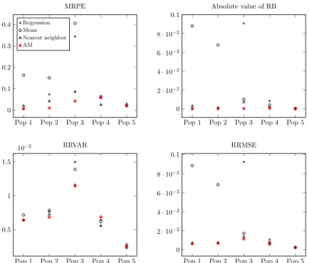
4.1 Comparison measures of four imputation methods in five popula-tions under SRSWOR. . . 82 4.2 Comparison measures of four imputation methods in five

popula-tions under stratified sampling. . . 83 5.1 Left panel: scatter plot of the auxiliary variable x against the

variable of interesty. Right panel: density estimate ofy. . . . 105 5.2 Density estimates of the income from the register (dashed curves)

and gaussian densities of three components (solid curves) for sampled units (top panel) and for respondents only (bottom panel).108

(14)

(15)

List of Tables

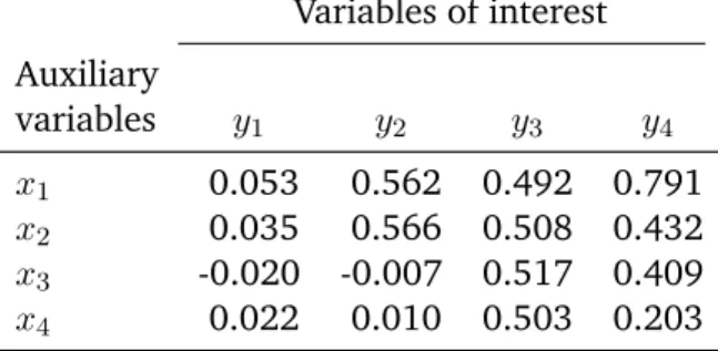
2.1 Correlations between the variables of interest and the balancing variables. . . 35 2.2 Ratio of the variance of the estimated total of the variables of

inter-est obtained using the new method (Algorithm 2.2) to the variance of the estimated total of the variables of interest obtained using Chauvet’s method with step 3 by landing phase by suppression of variables (Algorithm 2.1). . . 35 2.3 Mean time in seconds and failure rate of selection of a sample with

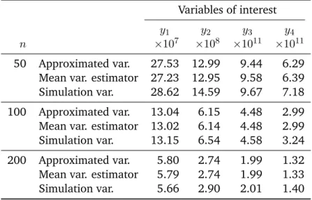
Chauvet’s method with step 3 by landing phase by suppression of variables (Algorithm 2.1) and with the new method (Algo-rithm 2.2) for 25, 50, 100, 250, 500, and 1,000 strata and 1 unit selected in each stratum with equal inclusion probabilities. . . 36 2.4 Approximated variance, mean of the variance estimator estimated

using 10,000 simulations, and variance obtained by 10,000 simu-lations in the case of the estimation of the total of 4 variables of in-terest using the new method (Algorithm 2.2). Three cases are con-sidered, namely the selection of samples of sizen= 50,100,200

respectively. . . 37 2.5 Relative root imputation variance (RRIV) of the imputed estimator

for a vector of domain means obtained through balanced random imputation using the new method (Algorithm 2.2). . . 38 3.1 Monte Carlo relative bias (RB), Monte Carlo relative root mean

square error (RRMSE), and Monte Carlo relative root imputa-tion variance (RRIV) for the total estimaimputa-tion, the 10-th percentile estimation, the 90-th percentile estimation, and the variance esti-mation of the variable of interestyin Case 1. . . 64 3.2 Monte Carlo relative bias (RB), Monte Carlo relative root mean

square error (RRMSE), and Monte Carlo relative root imputa-tion variance (RRIV) for the total estimaimputa-tion, the 10-th percentile estimation, the 90-th percentile estimation, and the variance esti-mation of the variable of interestyin Case 2. . . 65

(16)

3.3 Average over the simulations of the approximated conditional imputation variance of Expression (3.24), Monte Carlo imputation variance of the total and ratio of these two quantities in two

different cases. . . 66

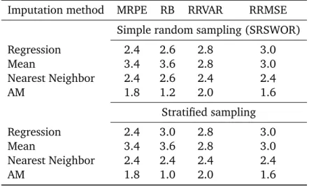
4.1 Average ranks over five populations of each imputation method for each measure of comparison (in absolute value). . . 84

4.2 Monte Carlo variance of the total, Monte carlo expectation of the bootstrap variance and coverage rate associated with AM imputation for two different sampling designs and five populations. 85 4.3 Comparison measures for four imputation methods for FES data. 85 4.4 Monte Carlo variance of the total, Monte carlo expectation of the bootstrap variance and coverage rate associated with AM imputation for FES data. . . 86

5.1 Comparison measures of estimators in Setting 1. . . 102

(17)

Introduction

Asurveyis a statistical method applied to study the characteristics of a popula-tion by examining only a part of this one called asample. In contrast with a survey, acensusis an exhaustive study of the characteristics of a population. Nonresponseoccurs when the desired information is only observed for a part of the sample and represents one of the sources of error the produced statistics are subject to. Nonresponse has two main consequences on the data. First, be-cause the number of observations is less than initially envisaged, nonresponse increases the variance of estimations. Second, nonresponse introduces a bias in the estimations if the recorded characteristics differ between respondents and nonrespondents.

Because official statistics are used within the decision-making process of au-thorities, they play an important role in the functioning of our society. The quality of the statistics produced by governmental agencies and other public agencies is therefore of fundamental importance. The control of the different sources of error in the survey contributes to this quality. As source of error, nonresponse is critical to this quest for quality and undeniably has to be given attention.

This document addresses the problem of nonresponse from a data processing and estimation point of view. Typically, we consider the perspective of a statistician who is given a sample survey data file containing missing values with the task of producing point and variance estimation. Imputation and reweighting procedures are proposed. This document does not cover any of the other aspects of nonresponse. For instance, we will not look at factors that influence nonresponse such as: the length or difficulty of items of the questionnaire, the method applied to collect the data, the period the data is collected, the nature of the subject of interest, or the characteristics of the interviewers. Neither will we focus on nonresponse follow-up procedures, which not only increase the response rate but also turn out to be useful when handling nonresponse by helping assess the similarities and dissimilarities between respondents and nonrespondents.

(18)

This document is organized as follows. Chapter1 proposes an overview of nonresponse in finite population sample surveys. It establishes the general framework of the research papers presented in this document. Chapters2to 5are self-contained papers submitted or published in peer-reviewed journals that have been developed in collaboration with different co-authors.

Chapter2is a reprint ofHasler and Tillé(2014) and presents an algorithm for stratified balanced sampling which is very fast, regardless of the number of strata. This algorithm turns out to be valuable for the purpose of the imputation method presented in Chapter3, as well as for many other applications, such as some large-scale surveys. In this chapter, we propose a variance estimator for the total and we illustrate one of the possible applications of the proposed algorithm.

Chapter3was co-written with Professor Yves Tillé and proposes a new random hot-deck imputation method. This method combines balanced sampling and a nonparametric approach. This results in an unbiased total estimator under very different models, providing protection against model misspecifiation. Moreover, the proposed method produces negligible imputation variance under specified hypotheses. In this chapter, we also suggest a formula to approximate the imputation variance of the total estimator, we describe the underlying models associated with the proposed method, and we study the asymptotic properties of the total estimator.

Chapter4was co-written with Professor Radu V. Craiu and presents a nonpara-metric method of imputation for item nonresponse in surveys. We consider smoothing splines models within an additive regression framework. This al-lows us to include a large number of auxiliary variables and to take advantage of some strong auxiliary information available. Because this method is non-parametric, it is very flexible and therefore provides protection against model misspecification in a wide range of problems. This chapter also suggests a bootstrap procedure to estimate the variance of the total.

Chapter5was developed in collaboration with Doctor Alina Matei and pro-poses three reweighting procedures for handling nonignorable nonresponse in surveys. We assume that the values of the variable of interest are sampled from a superpopulation which can be described as a mixture of some hid-den components or subpopulations. The response probabilities are modeled through logistic regression; the component structure of the variable of interest is considered in the model. The estimated response probabilities are used in a two-phase estimator of the population mean and an estimator of the variance of the mean is suggested.

(19)

This document closes with a general conclusion. Appendices contain technical elements relative to Chapter2and to Chapter3.

(20)

(21)

1

An introduction to finite

population sample

surveys and

nonresponse

Abstract

This chapter gives a brief overview of nonresponse in finite population sample surveys. It establishes the general framework of the research papers presented in Chapters3to 5. After general considerations pro-posed in Section1.1, Section1.2is devoted to estimation in the complete response case. Section1.3addresses nonresponse in the survey and is subdivided as follows. After having defined general concepts and notation of nonresponse, three types of nonresponse mechanisms are described in Section1.3.1. Then, Section1.3.2defines two levels of nonresponse and establishes two general handling approaches: reweighting procedures, further discussed in Section1.3.3, and imputation, further discussed in Section1.3.4.

Keywords: nonresponse mechanism, level of nonresponse, reweighting

procedure, imputation.

1.1 General considerations

Asample survey, often shortenedsurvey, is a statistical method applied to study the characteristics of a population by examining only a part of this one called a sample. By contrast, acensus survey, often shortenedcensus, is an exhaustive examination of the population. Because surveys require reduced cost and time of work compared to censuses, they represent an interesting option.

This document is concerned with finite population sampling, which studies the selection process of a sample in a population of finite size. In the finite population framework, all the units of the population are identifiable, which is not the case in the more classical infinite population framework. This particularity requires specific estimation tools, some of which being presented in this chapter.

A sampling process can be either probabilistic or non-probabilistic. It is re-ferred to as aprobabilistic samplingwhen the units are selected according to a random scheme and it is referred to as anon-probabilistic samplingotherwise. Probabilistic sampling is usually preferred by statisticians because, since units

(22)

are randomly selected, properties such as the estimated variability or bias are available. With non-probabilistic sampling, however, such properties are un-available. They are nevertheless circumstances in which probabilistic sampling is inapplicable, which explains the popularity of non-probabilistic sampling. This document focuses on probabilistic sampling and all the tools developed are limited to this context.

The central notion of this document isnonresponse, which means a failure to obtain responses from the sample; it corresponds to a missing data problem in the survey sampling framework. Despite all the actions taken to increase the response rate, nonresponse impairs most surveys. In contrast to the term nonresponse, the termcomplete nonresponse(orfull response) means a success to obtain all the responses from the sample.

Finally, a notion which plays a central role in the nonresponse framework and which will appear throughout this document is auxiliary information. This general notion includes any information not directly linked to the survey. Examples of auxiliary information are, but not limited to: the population total of a variable, the mean in a domain of a variable, or a variable with values known for all the population units or known for all the sampled units. Auxiliary information is used not only at the nonresponse treatment stage of the survey to reduce nonresponse error, but also at the design stage to improve the efficiency of sampling and at the estimation stage to construct accurate estimates. At the nonresponse treatment stage, strong auxiliary information explains the variability in the variable on interest, the variability in the nonresponse process, or, ideally, both simultaneously.

1.2 The complete response case

We consider a populationU ={1,2, . . . , i, . . . , N}of finite sizeN, where index

idenotes a generic unit of the population. Letybe a variable of interest and let

yi represent the value of the variable interest taken by uniti. The goal of the

survey is to estimate a parameter of interestθ, which is a function of the values

yi,i= 1, . . . , N of the variable of interest. Examples of parameters of interest

are, but not limited to: a population mean, a domain mean, a population quantile, a variance, or a regression coefficient. A common parameter of interest is the population total

Y =X

i∈U

yi.

A samplesis randomly selected without replacement from populationU using a probability distributionp(·)calledsampling design. A sampling design is a

(23)

probability distribution over all the possible samples in a population, i.e. a functionp(·)satisfying

• p(s)≥0for alls∈ S, • P

s∈Sp(s) = 1,

whereS is the set of all the possible samples in the population. The sample size, a random quantity, is the number of units contained in samples. It is denoted bynfor convenience but is understood asn(s) as it can differ from one sample to another. Thefirst order inclusion probabilityπi of unitiis the

probability that unitiappears in the selected sample, that is

πi = X

s∈S

s3i

p(s) = Pr (i∈s) = Pr (Ii= 1),

whereIi is the sample membership indicator

Ii = (

1 if unitiis selected in the sample,

0 otherwise.

It is supposed that a vectorx_i = (xi1, xi2, . . . , xiq)>ofq auxiliary variables is

known for each population unit or at least for each sampled unit. The values

yi of the variable of interest are recorded for each sampled unit. In the case of

complete response, the Horvitz-Thompson estimator (Horvitz and Thompson, 1952) b Y =X i∈s yi πi ,

is a design-unbiased estimator of the population totalY in the sense that, if

πi >0for all i∈U, it satisfiesEp(Yb) =Y, whereE_p is the expectation with

respect to the sampling design.

Before moving to nonresponse in the survey, let us briefly presenttwo-phase sampling, a notion which is, as we will mention below, closely related to non-response. Two-phase sampling consists of a double sampling and generalizes the simple one phase sampling described above. In a first phase, an initial samples1 is selected from populationU with a sampling designp1(·)and, in a

second phase, a subsamples2 is selected from the first phase samples1with a

sampling designp2(·|s1). A two-phase sampling design is useful when there is

unavailable or limited auxiliary information at the population level. In such circumstances, the first phase sampling is applied and auxiliary information is collected at the first phase sample level. The collected information then enhances the quality of estimates obtained from the second phase sampling. The values of the variable of interest are recorded for the units in the second phase samples2. Consider the first and second phase inclusion probabilities

(24)

π1i = Pr(i ∈ s1) and π2i = Pr(i ∈ s2|i ∈ s1;s1), respectively. Note that

the second phase inclusion probabilities are random variables since they de-pend on the observed values of the first phase sample. The double expansion estimator b YDE = X i∈s2 1 π1i 1 π2i yi (1.1)

generalizes the Horvitz-Thompson estimatorYb to two-phase sampling. This

estimator is design unbiased for the population totalY in the sense that, if

π1i, π2i>0for alli∈U,Ep(Yb_DE) = E₁E₂(Yb_DE|s₁) =Y, whereE₁andE₂are

the expectations with respect to the first and second phase sampling designs, respectively.

1.3 Nonresponse in the survey

Nonresponse is a failure to obtain responses from the sample, which partitions the sample into two subsets: the set of survey respondents and the set of survey nonrespondents. A sampled unitiis asurvey respondent(orrespondent) if its valueyiof the variable of interest is observed; it is asurvey nonrespondent(or nonrespondent) otherwise.

Nonresponse is a random process which represents a second phase of the survey: a sample of survey respondents is randomly selected from the initial sample. For a sampled uniti, the response indicator variableri, defined as

ri = (

1 if unitiis a survey respondent,

0 otherwise,

is a random quantity to be understood as the second phase sample membership indicator. Theresponse probabilityof a sampled unitiis the probabilitypi that

the unit is a survey respondent, that is

pi = P(ri = 1|i∈s;s).

Thenonresponse mechanismis the probability distributionq(·|s), whereq(sr|s)

is the probability of observing the setsr ={i∈s|ri = 1}of survey respondents.

The nonresponse mechanism describes the process that generates nonresponse. By analogy with two-phase sampling, the response probabilitiespirepresent the

inclusion probabilities of the second phase, the setsr of survey respondents is

the second phase sample, and the nonresponse mechanismq(·|s)corresponds to the second phase sampling design. The similarity between nonresponse and two-phase sampling is further discussed in Section1.3.3.

(25)

another. In this case, the nonresponse mechanism is described as follows: the response indicatorri is generated from a Bernoulli random variable with

parameterpi and the set of survey respondents is selected with a conditional

poisson sampling design, that is with the following probability distribution

q(sr|s) = Y

i∈s

pri

i (1−pi)1−ri.

1.3.1 Three types of nonresponse mechanisms

Three types of nonresponse mechanisms are distinguished: uniform, ignorable, and non-ignorable. Auniform nonresponse mechanismis a nonresponse mech-anism where each unit of the population has the same response probability

pi = p. It is in this case said that the data is missing completely at random

(MCAR).

A nonresponse mechanism is ignorable if the response probability pi does

not depend on the variable of interest once having taken into account any appropriate auxiliary information. The response indicator variable satisfies

Pr(ri = 1|x, y) = Pr(ri = 1|x). In the case of an ignorable nonresponse

mechanism, the data is said to be missing at random (MAR, seeRubin,1976). A uniform nonresponse mechanism is a particular case of ignorable nonresponse mechanism.

Finally, anon-ignorable nonresponse mechanismis a nonresponse mechanism which is not ignorable. There is a direct link between the response probability

pi and the variable of interest, and this link still holds once having taken into

account any appropriate auxiliary information. The data is in this case said to be not missing at random (NMAR).

Rubin (1976) set the foundation of the concept of ignorability. He defined conditions under which the process that causes the missing data can be ignored. Later,Little(1982) outlined models and provided a basis for the understanding of the effect of non-ignorable nonresponse on the survey estimates. The problems and estimation techniques associated with non-ignorable nonresponse mechanism have then become the subject of much research. Some of the the first research articles that tackled non-ignorable nonresponse mechanisms are Greenlees et al.(1982);Little(1983);Fay(1986).

1.3.2 Two levels of nonresponse and two handling approaches

There are two levels of nonresponse: unit (or total) nonresponse and item (or partial) nonresponse. Unit (or total) nonresponse is a complete lack of information on all the variables of interest for a given unit. Item(or partial) nonresponseis a lack of information on given variables of interest.

(26)

The main approaches to handle nonresponse are reweighting and imputation. Reweighting procedures consist, firstly, of eliminating the survey nonrespon-dents from the data file and, secondly, of increasing the initial weights of survey respondents in order to compensate for the eliminated units. SeeHaziza and Lesage(2015) for a discussion of reweighting procedures for unit nonresponse. Imputationprocedures consist of creating artificial values to fill in the gaps due to the missing values. SeeSande(1981a,b) for discussions of the problems associated with nonresponse and imputation.Single imputationmeans that a single artificial value is created for each missing value and, by contrast,multiple imputation(Rubin,1987) means that at least two artificial values are created for each missing value. In this document, we focus on single imputation. Generally, reweighting is applied to handle unit nonresponse and imputation is applied to handle item nonresponse. Reweighting is further discussed in Section1.3.3and single imputation is further discussed in Section1.3.4. 1.3.3 Reweighting for unit nonresponse

When reweighting for unit nonresponse, two types of approaches are mainly applied: response probabilities modeling or calibration. Withresponse probabil-ities modeling, nonresponse is viewed as a second phase of the survey. Let us suppose for the moment that the response probabilitiespi are known. By

anal-ogy with two-phase sampling, the double expansion estimator of Equation (1.1) suggests estimator e YP SA= X i∈sr 1 πi 1 pi yi.

SeeSärndal and Swensson(1987) for general results for two-phase sampling applied to the case of nonresponse. Similarly to the double expansion estimator, estimatorYe_{P SA}is unbiased for the population total under the assumptions that

πi >0 andpi > 0for alli∈ U, this latest being somewhat unrealistic since

some units are hardcore nonrespondents (Kott,1994). However, the response probabilities are unknown and a preliminary step consists of estimating them. A model for the response probabilities, called thenonresponse model, is supposed. From this model, we obtain estimated response probabilitiespbi. The estimated

response probabilities replace the true response probabilities in estimatorYe_{P SA}

and the propensity score adjusted estimator is obtained

b YP SA= X i∈sr 1 πi 1 b pi yi.

Three main estimation techniques applied to estimate the response probabilities are: parametric estimation, nonparametric estimation, and estimation with reweighting classes. With parametric estimation, a parametric nonresponse

(27)

model is assumed for the response probabilities

pi=f(xi,β),

where xi is a vector of auxiliary variables with values known for every

sam-pled unit and β is a vector of parameters. A method of estimation such as maximum likelihood is applied and an estimate βb of the vector of

parame-tersβ is obtained. The estimate βb is plugged in the nonresponse model to

obtain estimated response probabilitiespbi = f(xi,βb). Kim and Kim (2007)

showed that, with parametric estimation, the propensity score adjusted estima-torYb_{P SA}is generally more efficient than estimatorYe_{P SA}, which uses the true

response probabilities, provided that the parameters in the nonresponse model are estimated by maximum likelihood. With the second estimation technique, nonparametric estimation, we do not suppose a specific form for functionf in the nonresponse model. Rather, general characteristics such as smoothness are assumed. Because more flexible, nonparametric estimation is more robust to model misspecification than parametric estimation and is preferred when there is no prior idea of the form of functionf. Nonparametric estimation of the response probabilities for reweighting is considered inGiommi(1987); Niyon-senga(1994,1997); Da Silva and Opsomer(2006,2009). Finally, the third estimation technique, estimation with reweighting classes, consists of forming weighting classes based on auxiliary information. The response probabilities are then estimated by the response rate in each weighting class.Särndal and Swensson(1987) refer to these classes to as response homogeneity groups. SeeLittle(1986);Eltinge and Yansaneh(1997);Vartivarian and Little(2002) on the creation of weighting classes andKott(2012) on the use of the design weights. All three estimation techniques assume a nonresponse model. Mis-specification of this model implies a possibly severe bias of the propensity score adjusted estimatorYb_{P SA}.

With the second approach to reweighting,reweighting using calibration (see for instanceFolsom and Singh,2000;Särndal and Lundström,2005;Särndal, 2007;Kott,2006), we do not estimate the response probabilities. Rather, the design weights of respondents are adjusted to compensate for nonrespondents by means of calibration. With this approach, one distinguishes between two types of auxiliary variables: auxiliary variablesxU with valuesxU_i available for each respondent and with known population totalP

i∈UxUi , and auxiliary

variables xs with values xs_i available for each respondent and with known estimated total P

i∈sdixsi. Information coming from a register is a typical

example of the former type and paradata is a typical example of the latter type. The idea of reweighting using calibration is to find calibration weightswi as

close as possible (in an average sense for a given distance) to the initial design

(28)

weightsdi= 1/πi while respecting the calibration equation X i∈sr wixi=X, where xi = xU_i xs_i ! and X= P i∈UxUi P i∈sdixsi ! .

Note that this approach does not require the values of the auxiliary variables to be known for each population unit. Whereas calibrating at the sample level (variablesxsand lower part of the calibration equation) tends to correct the nonresponse error, calibrating at the population level (variablesxU and upper part of the calibration equation) tends to correct both the sampling error and the nonresponse error. The calibration weights are in the form

wi =diF(qix>i λ),

whereF is some function,λis some vector, andqiis a weight attached to unit

i. Several distance functions are proposed inDeville and Särndal(1992) as a means of measuring the distance between the initial design weightsdi = 1/πi

and the final weightswi, each of which providing a particular form for function

F (seeDeville and Särndal,1992, p. 378). An estimator of the total is then the calibrated estimator b YC = X i∈sr wiyi= X i∈sr 1 πi F(qix>i λ)yi.

Even though very different in spirit, there is a close parallel between the two aforementioned approaches to reweighting. The calibrated estimator Yb_C is

indeed a particular case of propensity score adjusted estimator Yb_{P SA} where b

pi = F(qixi>λ)−1. Hence, the calibrated estimator Yb_C can be thought as

a propensity score adjusted estimator where the response probabilities are estimated via calibration.

When reweighting using generalized calibration (Deville,2000,2002;Kott, 2006) or using generalized raking procedures (seeDeville et al.,1993) instead of calibration, one allows for the variables that appear in the final weights to differ from the variables that appear in the calibration equation. One finds calibration weights in the form

wG_i =diF(qiz>i λ),

(29)

for each survey respondent, while respecting the calibration equation

X

i∈sr

wG_i xi=X.

An estimator of the total is then thegeneralized calibration estimator

b YGC = X i∈sr w_iGyi= X i∈sr 1 πi F(qiz>i λ)yi.

Similarly to the calibrated estimator, the generalized calibration estimator can be thought as a propensity score adjusted estimator where the response probabilities are estimated nonparametrically via generalized calibration and

b

pi = F(qiz>i λ)−1. Traditionally, vectors xi and zi are assumed to have the

same dimension but a solution was proposed to handle the case of different dimensions (Chang and Kott,2008). Reweighting using generalized calibration is applied to handle non-ignorable nonresponse (Deville,2000;Kott and Chang, 2010). The variable of interest is included in the instrumental variables; the effect of the variable of interest on the response probabilities comes into the equation. Particular care should be taken when reweighting for unit nonresponse with generalized calibration: Lesage and Haziza(2015) highlight the risks of bias and variance amplification of the generalized calibration estimator.

1.3.4 Imputation for item nonresponse

Reweighting is usually avoided to handle item nonresponse because it requires many sets of weights for some large number of variables. Rather, imputation is preferred. Imputation is simple in the sense that it generates a complete data file which is available to estimate all parameters of interest. However, particular attention should be paid when handling a data file containing im-puted values. Such values are artificial and considering them as observed produces invalid variance estimators and invalid inference. There is an ex-tensive literature devoted to variance estimation and inference with imputed data, see for instance Rao (1990); Särndal (1990); Rao and Shao (1992); Lee et al.(1994);Rao and Sitter(1995);Fay(1996);Rao(1996);Shao and Sitter(1996); Kim(2001);Brick et al. (2004);Haziza and Rao(2006). An effective imputation method should impute consistent values; some procedures consist of imputing manually based on logical rules or automatically based on a systematic approach (Fellegi and Holt,1976).

Imputation methods are classified into two groups: deterministic imputation methods and random imputation methods. For fixed sample and fixed set of survey respondents, deterministic imputation methods produce the same imputed values if the imputation is repeated in the same sample and in the

(30)

same set of survey respondents. Examples of deterministic imputation are: ratio imputation (seeDavid and Sukhatme,1974;Rao and Sitter,1995;Shao,2000; Kim and Park, 2006), regression imputation, respondent mean imputation, nearest neighbor imputation (studied in Rancourt et al., 1994; Chen and Shao,1997,2000,2001;Shao and Wang,2008;Shao,2009), predictive mean matching (Little, 1988), and auxiliary value imputation (Beaumont et al., 2011). Random imputation methodshave, as indicated by their name, a random component. As a result, they produce, for fixed sample and fixed set of survey respondents, different imputed values if the imputation is repeated. Examples of random imputation methods are: random hot-deck imputation, imputation with added residuals (Chen et al.,2000;Chauvet et al.,2011b), and fractional hot-deck imputation (Kim and Fuller,2004). Unlike deterministic imputation methods, random imputation methods tend to preserve the distribution of the variable being imputed at the expense of an additional variance in estimations which is called theimputation variance. Many authors have been interested in minimizing the imputation variance, see for instanceKalton and Kish(1981, 1984); Chen et al. (2000); Kim and Fuller (2004); Fuller and Kim (2005); Chauvet et al.(2011b).

Alternatively, imputation methods can be classified as either donor or predicted value. Donor imputation methodsreplace the missing value of a survey non-respondent with an observed value. The unit providing the value is called a donorand the unit receiving the value is called arecipient. Examples of donor imputation methods are: random hot-deck imputation, nearest neighbor impu-tation, and previous value imputation. Predicted value imputation methodsuse functions of the observed values of survey respondents to predict the missing values of survey nonrespondents. Examples of predicted value imputation methods are: ratio imputation, regression imputation, and respondent mean imputation.

In Section 1.3.3, when reweighting using response probabilities modeling, we assumed a model for the response probabilities, the nonresponse model. When imputing, we rather assume a model for the variable of interest, the imputation model (Kalton and Kasprzyk, 1986; Särndal, 1992). From this model, an imputed valuey_i∗ is obtained for each survey nonrespondentiand theimputed estimator

b YI = X i∈s 1 πi [yiri+yi∗(1−ri)]

is considered. Every imputation method assumes an imputation model, either defined clearly or underlain. Misspecification of this model implies a possibly severe bias of estimatorYb_I.

(31)

Parametric and nonparametric imputation models are considered. In a para-metric framework, we consider a general imputation model

yi =f(xi,β) +εi,

wheref is a specified function,xi is a vector of auxiliary variables with values

known for every sampled unit, β is a vector of parameters, andεi are

zero-mean independent errors with varianceσ_i2. For deterministic imputation, an imputed valuey_i∗for a survey nonrespondentiis obtained as follows:

y_i∗=f(xi,βb_r),

whereβb_r is an estimate ofβbased on the observed valuesy_i andx_i of survey

respondents. For random imputation, a random residual ε∗_i is added, i.e.

y_i∗ =f(xi,βb_r) +ε∗_i. Some examples of imputation methods which assume a

parametric imputation model are: regression imputation, mean imputation, and ratio imputation. In a nonparametric framework, we do not specify the form of function f or the structure of the variance σ_i2. Some examples of imputation methods which assume a nonparametric imputation model are: nearest neighbor imputation and predictive mean matching.

(32)

(33)

2

Fast balanced sampling

for highly stratified

populations

Abstract

Balanced sampling is a very efficient sampling design when the variable of interest is correlated to the auxiliary variables on which the sample is balanced. A procedure to select balanced samples in a stratified pop-ulation has previously been proposed. Unfortunately, this procedure becomes very slow as the number of strata increases and it even fails to select samples for some large numbers of strata. A new algorithm to select balanced samples in a stratified population is proposed. This new procedure is much faster than the existing one when the number of strata is large. Furthermore, this new procedure makes it possible to select samples for some large numbers of strata, which was impossible with the existing method. Balanced sampling can then be applied on a highly stratified population when only a few units are selected in each stratum. Finally, this algorithm turns out to be valuable for many applications as, for instance, for the handling of nonresponse.1

Keywords: balanced sampling, stratified sampling, cube method,

un-equal probability sampling, auxiliary information.

2.1 Introduction

Auxiliary information is a central point in survey statistics. It is widely-used in a large set of sampling designs. For instance, auxiliary information can be used to select stratified samples; it can also be used to define sampling designs with unequal probabilities. Regardless of the way auxiliary information is used, the main goal is to improve the quality of the estimates.

A stratified sampling design consists of dividing the population into subgroups (thestrata) and of selecting samples in each stratum. Auxiliary information must be available to define the strata. The way the population has to be stratified is not always clear. A lot of research has been conducted on this topic. Neyman (1934) looked into optimum allocation. A method for the iterative improvement of the points of stratification was given and illustrated in Dalenius and Hodges(1959). Bülher and Deutler(1975) presented a method

1_{This article is a reprint of Hasler, C. and Tillé, Y. (2014).} _{Fast balanced sampling}

for highly stratified population. Computational Statistics & Data Analysis, 74:81–94.

http://dx.doi.org/10.1016/j.csda.2013.12.005

(34)

to determine a global optimal solution by linear programming whereasLavallée and Hidiroglou(1988) tackled the issue of stratification of a highly skewed population. Díaz-García and Garay-Tápia (2007) considered the allocation problem in stratified surveys as a problem of stochastic programming. Stratified sampling designs have the interesting property of reducing the variance of the Horvitz-Thompson estimator compared to unstratified sampling designs if the values of the variable of interest are somewhat homogenous inside the strata.

A balanced sampling design consists of selecting samples in such a way that the Horvitz-Thompson estimator for some auxiliary variables matches the population total. These auxiliary variables are called thebalancing variables. Deville et al.(1988) described a method to obtain balanced samples and, later, the cube method (Deville and Tillé,2004) was proposed for the same purpose. Some methods have been proposed for the computing of optimal inclusion probabilities for balanced sampling as for instance those given in Tillé and Favre (2005),Nedyalkova and Tillé(2008), and Chauvet et al.(2011a). A balanced sampling design is a very efficient sampling design when the variable of interest is correlated to the balancing variables.

In the presence of auxiliary variables correlated to the variable of interest and in the presence of strata, it is thus very useful to select samples applying a procedure which produces both stratified and balanced samples. Brewer (1999), indeed, showed that balanced sampling inside the strata can consider-ably improve the robustness and efficiency of some estimates. Chauvet(2009) proposed a stratified balanced sampling procedure: his algorithm selects sam-ples which are approximately balanced in each stratum, balanced across the entire population and such that the sample size is fixed in each stratum. Unfor-tunately, Chauvet’s procedure can be slow when the number of strata is large. In this paper, a new algorithm for stratified balanced sampling is proposed. This algorithm is much faster than Chauvet’s algorithm when the number of strata is large.

The proposed algorithm turns out to be valuable for many applications, namely the selection of balanced samples in highly stratified populations when only a few units are selected in each stratum. For example, the proposed algorithm could improve the quality of estimates produced by some large-scale surveys. Indeed, in some large-scale multistage surveys, only one or two primary sam-pling units or first-stage units are selected in each stratum and the number of strata can be very large. Besides, the proposed method can also be used to treat nonresponse. Stratified sampling has long been used for the purpose of imputation. For instance, Kalton and Kish(1984) had already proposed selecting stratified sample of respondents to act as donors in order to reduce imputation variance. This idea can be extended by using the proposed method

(35)

for stratified balanced sampling. Indeed,Chauvet et al.(2011b) proposed a class of imputation methods that they called balanced random imputation and which use balanced sampling. This class of method is constructed such that the imputation variance is eliminated. Furthermore, the imputed values can be obtained through stratified balanced sampling. In this framework, however, the considered number of strata may be very large, hence the proposed method for stratified balanced sampling turns out to be useful in this context.

The paper is organized as follows. In Section 2.2, notions and concepts of balanced sampling are reviewed. Then in Section 2.3, Chauvet’s method is described. The new method is presented in Section 2.4. A solution to apply the new method in cases where the sum of the inclusion probabilities is not an integer in each stratum is given in Section2.5. Section2.6focusses on estimation of the variance of the Horvitz-Thompson estimator whereas Section2.7presents a possible application of the new method to the handling of nonresponse. Brief simulation studies were conducted to test the performance of the new sampling algorithm, to test the accuracy of the proposed formulas for the variance, and to illustrate the application of the new sampling algorithm in the context of handling of nonresponse. The results of these studies are given in Section 2.8. Finally, Section 2.9 closes the paper with concluding remarks.

2.2 Balanced sampling

Consider a finite population U = {1, . . . , k, . . . , N} of size N in which the aim is to select a random sampleS, i.e. a subset of the population randomly selected. A sampling designp(·)assigns to each subsets⊂U a probabilityp(s)

of being selected with

X

s⊂U

p(s) = 1.

The inclusion probabilityπkis the probability of selecting a particular unitk.

The aim is to estimate a total

ty = X

k∈U

yk,

for some variable of interesty. Ifπk >0 for allk ∈U,then theHorvitz and

Thompson(1952) estimator given by

b ty = X k∈S yk πk , is unbiased forty.

Consider now that a column vectorxk∈Rq of auxiliary variables is available

(36)

for all the unitsk∈U. A sampling designp(·)with inclusion probabilitiesπkis said to be balanced onx_kif X k∈s x_k πk = X k∈U x_k, (2.1)

for every subset s ⊂ U such that p(s) > 0. In many cases, it is not possi-ble to find a subset s ⊂ U satisfying exactly equation (2.1). As a result, a sampling designp(·) can often not be exactly balanced. This problem is re-ferred to as arounding problem. Consider the sample membership indicators

s= (s1 . . . sk . . . sN)>where

sk= (

1 ifk∈S,

0 ifk6∈S.

When a rounding problem is encountered, it is not possible to find a vectorsof zeros and ones that exactly satisfies the equation

X k∈U x_k πk sk= X k∈U x_k.

Deville and Tillé (2004) proposed the cube method, which allows for the selection of balanced samples. The cube method is an algorithm composed of two phases: theflight phaseand the landing phase. In what follows, the results given by the two phases of the algorithm are presented. The aim is not to describe the cube method in detail but only the outputs of both phases.

• The flight phase provides a vector of random variables

φ= (φ1 . . . φk . . . φN)>, with0≤φk≤1, such that (i) E(φk) =πk for allk∈U,

(ii) X k∈U x_k πk φk= X k∈U x_k,

(iii) #{k|0< φk<1} ≤q,whereqis the dimension ofxk.

A unitkwithφk = 1is selected in the sample and a unitkwithφk = 0

is definitely rejected. Whether there is a rounding problem or not, the equation in(ii)is exactly satisfied. In the presence of a rounding problem and as explained at the end of the previous paragraph, it is, however, not possible to find a vectorφof zeros and ones which is a solution to the equation in(ii). In that case, someφk’s are not integers and some units

are not yet selected or rejected at the end of the flight phase. It is possible to show, as stated in(iii), that the number of non-integerφk’s is at mostq.

In other words, at mostqunits are not yet selected or rejected at the end of the flight phase.Chauvet and Tillé(2006) proposed a fast algorithm for the flight phase. In what follows, the flight phases are carried out by means of this algorithm.

(37)

• The landing phase is used to deal with the rounding problem. Its main idea is to relax the balancing constraint in order to address the problem of the units that have not yet been rejected or selected at the end of the flight phase. The landing phase provides a vectors= (s1 . . . sk . . . sN)>of

sample membership indicator such that (i) E(sk|φ) =φkfor allk∈U,

(ii) X k∈U x_k πk sk≈ X k∈U x_k.

A unitkwithsk= 1is selected in the sample and a unitkwithsk= 0is

rejected. At the end of the landing phase, every unit has been selected or rejected. Deville and Tillé(2004) have proposed two ways of running the landing phase: by linear programming or by suppression of variables. The landing phase by linear programming consists of solving a linear programming problem through the simplex algorithm. The list of all possible samples from a population of sizeq, whereqis the dimension of

x_k, must be generated and this can be impossible whenq exceeds a limit. Therefore, the landing phase by linear programming cannot be applied when the number of auxiliary variables q exceeds this limit, which is generally 20.

When one of the variables inx_kis equal or proportional toπk,the balancing

constraint (2.1) implies that

X k∈s πk πk = X k∈U πk⇔n(s) = X k∈U πk,

wheren(s)is the size of the subsets⊂U. This means that the sampling design has a fixed sample size. This equality can only be exactly satisfied if the sum of the inclusion probabilities is an integer. If the sum of the inclusion probabilities is not an integer, then the cube method usually selects a sample whose size is the smallest integer larger than this sum or the largest integer smaller than this sum.

2.3 Chauvet’s method for stratified balanced sampling

The population is presumed to be partitioned intoH nonoverlapping strata

U1, . . . , Uh, . . . , UH. Let1(k∈Uh)be the stratum membership indicator that

takes value 1 if unit k belongs to stratum h and 0 otherwise. A stratified balanced sampling designp(·)is a sampling design which is balanced onxkin

each stratum, i.e.

X k∈s∩Uh x_k πk = X k∈Uh x_k,

for eachs⊂U withp(s)>0and for eachh= 1, . . . , H.

Suppose that the goal is to balance onxk∈Rqsuch that none of the auxiliary

(38)

variables is proportional toπk. Chauvet’s method (Chauvet,2009) is presented

in Algorithm2.1. The main idea of this method is to first run flight phases independently inside the strata. This ensures that the samples are as balanced as possible within the strata. Next, in a second step, a general flight phase is run on all the units of the population that have not yet been selected or rejected at the end of the first step. It results in samples that are as balanced as possible across the entire population. Finally, a third step is carried out to handle the case of units that have not yet been rejected or selected at the end of the second step. Originally inChauvet(2009), the third step consisted of unequal probability sampling whereas the third step of the new procedure presented in Section2.4consists of a landing phase by suppression of variables. A landing phase by suppression of variables takes the balancing constraint into account and therefore provides more accurate estimates than unequal probability sampling. Henceforth, for a fair comparison between methods with respect to the accuracy of the estimates and as pointed out by one of the referees, the third step of Chauvet’s algorithm has here been modified onto a landing phase by suppression of variables.

Algorithm 2.1Chauvet stratified balanced sampling with step 3 by landing phase by suppression of variables

Step 1: Carry out a flight phase, with balancing variables (πk x>k)

> _and

inclusion probabilitiesπkindependently in each stratumUh.

Step 1 provides vectorφofφk’s.

Step 2: Carry out a flight phase, with balancing variables

φk1(k∈U1) . . . φk1(k∈Uh) . . . φk1(k∈UH)

φkx>k

πk !>

and inclusion probabilitiesφkon the set of units with non-integerφk,

i.e. on the units that are not yet selected or rejected at the end of step 1.

Step 2 provides vectorψ ofψk’s.

Step 3: Do a landing phase with inclusion probabilities ψk and balancing

variables

ψk1(k∈U1) . . . ψk1(k∈Uh) . . . ψk1(k∈UH)

ψkx>k

πk !>

on the set of units with non-integer ψk. Use the landing phase by

suppression of variables.

In step 1 of Algorithm2.1,q+ 1balancing variables are considered in each flight phase. Therefore at mostq+ 1units in each stratum are not yet selected or rejected at the end of step 1. As a result, step 2 concerns at most(q+ 1)H

(39)

It may be impossible to carry out the flight phase of step 2 if the considered design is highly stratified (i.e. ifHis very large). Indeed, the fast algorithm for the flight phase proposed by Chauvet and Tillé(2006) requires the use of a matrix that is equal in size to the number of balancing variables times the number of balancing variables plus one. However, this approach can only be used with matrices of a limited size. This limit depends on the computer. If a highly stratified design is considered, the flight phase of step 2 requires the use of a huge matrix and it may be impossible to carry it out. Henceforth, Algorithm2.1is likely to fail for highly stratified designs.

2.4 New procedure for highly stratified balanced sampling

In this section, it is supposed that the sum of the inclusion probabilities in each stratum

X

k∈Uh

πk=nh,

is an integer. This hypothesis will be relaxed in Section2.5but will considerably simplify the complexity of the proposed algorithm. The main idea of the proposed method described in Algorithm 2.2, is to first run a flight phase independently in each stratum. Then, in a second step,U1 andU2 are merged

and a flight phase is run. Next,U1andU2are merged withU3and a flight phase

is run again and so on. Finally, a landing phase by suppression of variables is carried out in a third step.

This alternative implementation might look like a simple variant but it actually offers major advantages. An important advantage is that it greatly reduces computation time when some large numbers of strata are considered. This reduction in computation time is explained in what follows. In step 2 of Algorithm2.2, the flight phases are carried out with the balancing variables

z(j)_k . Consider matrix Z(j) whose rows are thez(j)_k > restricted to the kwith non-integerφ(j_k−1), i.e. theksuch that0< φ(j_k−1)<1.

Property 2.1 With Algorithm2.2, forj= 2, . . . , H

(i) #    k∈ j [ i=1 Ui 0< φ (j) k <1    ≤2q+ 2,

(ii) the number of non-null columns of matrixZ(j)is less than or equal to2q+ 2, where a null column is a column that contains only zeros.

The proof is given in AppendixAand requires that the sum of the inclusion probabilities is an integer in each stratum. In light of Property2.1, it appears that the flight phase must never be applied on a matrix of balancing variables with more than2q+ 2columns with Algorithm2.2because the null columns can be removed. However the flight phase could be applied on a matrix of balancing variables with up toq+H columns with Algorithm2.1. This size

(40)

Algorithm 2.2New procedure for highly stratified balanced sampling

Step 1: Carry out a flight phase, with balancing variables (πk x>k)

> _and

inclusion probabilitiesπkindependently in each stratumUh.

Step 1 provides vectorφ(1)ofφ(1)_k ’s.

Step 2: Forj= 2toH:

• Carry out a flight phase on the union of strataU1, . . . , Uj, with

balancing variables z(j)_k = φ(j_k−1)1(k∈U1) . . . φ(j −1) k 1(k∈Uj) φ(j_k−1)x>_k πk !>

and inclusion probabilitiesφ(j_k−1) on the set of units with non-integerφ(j_k−1). The flight phase provides a vectorφ(j) of φ(j)_k ’s for units with non-integerφ(j_k−1).

• Setφ(j)_k =φ_k(j−1) for units with integerφ(j_k−1). Step 2 provides vectorφ(H)ofφ(H)_k ’s.

Step 3: Do a landing phase with inclusion probabilitiesφ(H)_k and balancing variables z(H+1)_k = φ(H_k )1(k∈U1) . . . φ (H) k 1(k∈UH) φ(H_k )x_k> πk !>

on the set of units with non-integerφ(H)_k . Use the landing phase by suppression of variables.

difference of the matrices considered in the flight phases affects the execution time of the algorithms. Indeed, even if Algorithm2.2requires us to run2H−1

flight phases against only H+ 1 for Algorithm 2.1, Algorithm2.2 becomes much faster than Algorithm 2.1 as H increases. Even more interesting is the fact that Algorithm 2.2 is much more resistent to numerical instability than Algorithm 2.1 thanks to the reduction in size stated above. Indeed, numerical instability increases when the dimension of the matrices to deal with increases. In step 2 of Algorithm2.1, flight phases operate with matrices of up to(q+H)×(q+H+ 1)in size whereas flight phases operate with matrices of up to(2q+ 2)×(2q+ 3)in size in step 2 of Algorithm2.2. As this dimension depends onHfor Algorithm2.1, numerical instability increases asH increases. This is not the case with Algorithm2.2.

Another advantage of the proposed method is that a landing phase can be applied in the last step even if the population is highly stratified. Indeed, at the last loop of step 2, we have

#nk∈U 0< φ (H) k <1 o ≤2q+ 2.

(41)

This implies that the last step concerns at most2q+ 2 units. This quantity is independent of the number of strata H. Consequently, a landing phase can be applied in step 3 regardless of the number of strata. Therefore, the balancing can be taken into consideration in step 3 of Algorithm2.2even if the population is highly stratified. As far as the last step of Algorithm2.1is concerned, a landing phase may not be applied for highly stratified populations as the number of units considered can reachq+H. The landing phase of step 3 of Algorithm2.2must be done by suppression of variables in order to ensure fixed size sampling inside the strata. Indeed, steps 1 and 2 of Algorithm2.2 consist of flight phases. The balancing equations of the carried out flight phases imply that

X

k∈Uh

φ(j)_k =nh,

for each j = 1, . . . , H and each h = 1, . . . , H. In particular, the following equation

X

k∈Uh

φ(H)_k =nh, (2.2)

is satisfied for eachh= 1, . . . , H. In step 3 of Algorithm2.2, a landing phase is carried out. The aim is to derive a samplesofsk’s. The balancing equations

linked to the firstHbalancing variablesφ(H_k )1(k∈Uh),h= 1, . . . , Hsimplify

to X k∈Uh sk = X k∈Uh φ(H)_k , (2.3)

forh= 1, . . . , H. Combining Equation (2.2) together with Equation (2.3) leads to

X

k∈Uh

sk =nh, (2.4)

for h = 1, . . . , H. As nh is in this section supposed to be an integer,

equa-tion (2.4) can always be satisfied; all that is required is to select nh units in

each stratum Uh. The landing phase by suppression of variables consists of

alternate dropping the last balancing variables and running a flight phase again until the remaining constraints are exactly satisfied. As explained above, the constraints linked to the first balancing variablesφ(H)_k 1(k∈Uh),h= 1, . . . , H,

can always be satisfied. As the landing phase is carried out by suppression of variables in step 3 of Algorithm2.2, only the lastq variables

φ(H)_k x>_k

πk

are suppressed and fixed size sampling inside the strata is ensured.

Furthermore, the selected samples= (s1 . . . sk . . . sN)>satisfiesE(sk) =πk.

To summarize, the sampling design associated with Algorithm2.2is balanced,

(42)

can be highly stratified and ensures fixed size sampling within the strata. Selection of samples with highly stratified designs becomes tractable with this new procedure.

Parallel computing can be used to slightly speed up both Algorithm2.1and Algorithm2.2. Firstly, it is conceivable to carry out the flight phases of steps 1 of both Algorithms in parallel. It is also possible to adapt step 2 of Algorithm2.2 to use parallel computing. Indeed, even though it is impossible to roughly apply parallel computing as iterative procedures are involved, step 2 can be adapted for it as follows. The procedure proposed in step 2 of Algorithm2.2 can be applied in parallel on non-overlapping groups of strata first. Then some of these groups can be gathered and the same procedure can be used, and so on.

Finally, Algorithm2.1and Algorithm2.2can both be applied if the number of ba