SAS 9.3 SQL Procedure

(1)

SAS

®

9.3 SQL Procedure

User’s Guide

(2)

SAS® 9.3 SQL Procedure User’s Guide

For a hardcopy book: No part of this publication may be reproduced, stored in a retrieval system, or transmitted, in any form or by any means,

electronic, mechanical, photocopying, or otherwise, without the prior written permission of the publisher, SAS Institute Inc.

For a Web download or e-book:Your use of this publication shall be governed by the terms established by the vendor at the time you acquire this

publication.

The scanning, uploading, and distribution of this book via the Internet or any other means without the permission of the publisher is illegal and punishable by law. Please purchase only authorized electronic editions and do not participate in or encourage electronic piracy of copyrighted materials. Your support of others' rights is appreciated.

U.S. Government Restricted Rights Notice: Use, duplication, or disclosure of this software and related documentation by the U.S. government is

subject to the Agreement with SAS Institute and the restrictions set forth in FAR 52.227–19 Commercial Computer Software-Restricted Rights (June 1987).

SAS Institute Inc., SAS Campus Drive, Cary, North Carolina 27513. 1st printing, July 2011

2nd printing, August 2012

SAS®_{Publishing provides a complete selection of books and electronic products to help customers use SAS software to its fullest potential. For} more information about our e-books, e-learning products, CDs, and hard-copy books, visit the SAS Publishing Web site at

support.sas.com/publishing or call 1-800-727-3228.

SAS®_{and all other SAS Institute Inc. product or service names are registered trademarks or trademarks of SAS Institute Inc. in the USA and other} countries. ® indicates USA registration.

(3)

SQL Procedure Reference

207 Chapter 7 • SQL Procedure . . . 209

Overview . . . 210

Syntax: SQL Procedure . . . 212

Examples: SQL Procedure . . . 245

Chapter 8 • SQL SELECT Statement Clauses . . . 291

Dictionary . . . 291

Chapter 9 • SQL Procedure Components . . . 305

Overview . . . 305

PART 3

Appendixes

359 Appendix 1 • SQL Macro Variables and System Options . . . 361

Appendix 2 • PROC SQL and the ANSI Standard . . . 373

Appendix 3 • Source for SQL Examples . . . 379

Overview . . . 379

EMPLOYEES . . . 379

HOUSES . . . 380

MATCH_11 . . . 380

(5)

PROCLIB.HOUSES . . . 382 PROCLIB.MARCH . . . 383 PROCLIB.PAYLIST2 . . . 384 PROCLIB.PAYROLL . . . 384 PROCLIB.PAYROLL2 . . . 387 PROCLIB.SCHEDULE2 . . . 388 PROCLIB.STAFF . . . 388 PROCLIB.STAFF2 . . . 391 PROCLIB.SUPERV2 . . . 391 STORES . . . 392 SURVEY . . . 392 Glossary . . . 393 Index . . . 397 Contents v

(6)

(7)

About This Book

Syntax Conventions for the SAS Language

Overview of Syntax Conventions for the SAS Language

SAS uses standard conventions in the documentation of syntax for SAS language elements. These conventions enable you to easily identify the components of SAS syntax. The conventions can be divided into these parts:

• syntax components • style conventions • special characters

• references to SAS libraries and external files

Syntax Components

The components of the syntax for most language elements include a keyword and arguments. For some language elements, only a keyword is necessary. For other language elements, the keyword is followed by an equal sign (=).

keyword

specifies the name of the SAS language element that you use when you write your program. Keyword is a literal that is usually the first word in the syntax. In a CALL routine, the first two words are keywords.

In the following examples of SAS syntax, the keywords are the first words in the syntax:

CHAR (string, position) CALL RANBIN (seed, n, p, x); ALTER (alter-password) BEST w.

REMOVE <data-set-name>

In the following example, the first two words of the CALL routine are the keywords: CALL RANBIN(seed, n, p, x)

The syntax of some SAS statements consists of a single keyword without arguments: DO;

... SAS code ...

(8)

END;

Some system options require that one of two keyword values be specified: DUPLEX | NODUPLEX

argument

specifies a numeric or character constant, variable, or expression. Arguments follow the keyword or an equal sign after the keyword. The arguments are used by SAS to process the language element. Arguments can be required or optional. In the syntax, optional arguments are enclosed between angle brackets.

In the following example, string and position follow the keyword CHAR. These arguments are required arguments for the CHAR function:

CHAR (string, position)

Each argument has a value. In the following example of SAS code, the argument string has a value of 'summer', and the argument position has a value of

4:x=char('summer', 4);

In the following example, string and substring are required arguments, while modifiers and startpos are optional.

FIND(string, substring <,modifiers> <,startpos>

Note: In most cases, example code in SAS documentation is written in lowercase with a monospace font. You can use uppercase, lowercase, or mixed case in the code that you write.

Style Conventions

The style conventions that are used in documenting SAS syntax include uppercase bold, uppercase, and italic:

UPPERCASE BOLD

identifies SAS keywords such as the names of functions or statements. In the following example, the keyword ERROR is written in uppercase bold: ERROR<message>;

UPPERCASE

identifies arguments that are literals.

In the following example of the CMPMODEL= system option, the literals include BOTH, CATALOG, and XML:

CMPMODEL = BOTH | CATALOG | XML

italics

identifies arguments or values that you supply. Items in italics represent user-supplied values that are either one of the following:

• nonliteral arguments In the following example of the LINK statement, the argument label is a user-supplied value and is therefore written in italics: LINK label;

• nonliteral values that are assigned to an argument

In the following example of the FORMAT statement, the argument DEFAULT is assigned the variable default-format:

(9)

Items in italics can also be the generic name for a list of arguments from which you can choose (for example, attribute-list). If more than one of an item in italics can be used, the items are expressed as item-1, ..., item-n.

Special Characters

The syntax of SAS language elements can contain the following special characters: =

an equal sign identifies a value for a literal in some language elements such as system options.

In the following example of the MAPS system option, the equal sign sets the value of MAPS:

MAPS = location-of-maps < >

angle brackets identify optional arguments. Any argument that is not enclosed in angle brackets is required.

In the following example of the CAT function, at least one item is required: CAT (item-1 <, ..., item-n>)

|

a vertical bar indicates that you can choose one value from a group of values. Values that are separated by the vertical bar are mutually exclusive.

In the following example of the CMPMODEL= system option, you can choose only one of the arguments:

CMPMODEL = BOTH | CATALOG | XML ...

an ellipsis indicates that the argument or group of arguments following the ellipsis can be repeated. If the ellipsis and the following argument are enclosed in angle brackets, then the argument is optional.

In the following example of the CAT function, the ellipsis indicates that you can have multiple optional items:

CAT (item-1 <, ..., item-n>) 'value' or “value”

indicates that an argument enclosed in single or double quotation marks must have a value that is also enclosed in single or double quotation marks.

In the following example of the FOOTNOTE statement, the argument text is enclosed in quotation marks:

FOOTNOTE <n> <ods-format-options 'text' | “text”>; ;

a semicolon indicates the end of a statement or CALL routine.

In the following example each statement ends with a semicolon: data namegame; length color name $8; color = 'black'; name = 'jack'; game = trim(color) || name; run;

(10)

References to SAS Libraries and External Files

Many SAS statements and other language elements refer to SAS libraries and external files. You can choose whether to make the reference through a logical name (a libref or fileref) or use the physical filename enclosed in quotation marks. If you use a logical name, you usually have a choice of using a SAS statement (LIBNAME or FILENAME) or the operating environment's control language to make the association. Several methods of referring to SAS libraries and external files are available, and some of these methods depend on your operating environment.

In the examples that use external files, SAS documentation uses the italicized phrase file-specification. In the examples that use SAS libraries, SAS documentation uses the italicized phrase SAS-library. Note that SAS-library is enclosed in quotation marks:

infile file-specification obs = 100; libname libref 'SAS-library';

(11)

What’s New in the SAS 9.3 SQL

Procedure

Overview

PROC SQL reference information from the Base SAS Procedures Guide and SAS SQL system options from the SAS Language Reference: Dictionary have been moved to this book, SAS SQL Procedure User’s Guide. This enables our customers to access PROC SQL information in one location. The following are new features and enhancements: • ability to optimize the PUT function

• ability to reuse the LIBNAME statement database connection • additional PROC SQL statement options

• additional macro variable specifications for the INTO clause • additional dictionary table

• additional system macro variable • updated output examples

In the second maintenance release for SAS 9.3, the following enhancements have been made:

• modified the default value for the SQLGENERATION= option • added security for password-protected SAS views

Ability to Optimize the PUT Function

The following reduce PUT options and system options have been modified to optimize the PUT function:

• REDUCEPUTOBS= • REDUCEPUTVALUES= • SQLREDUCEPUTOBS= • SQLREDUCEPUTVALUES=

(12)

Ability to Reuse the LIBNAME Statement

Database Connection

The database connection that is established with the LIBNAME statement can be reused in the CONNECT statement. The keyword USING has been added to implement this feature.

Additional PROC SQL Statement Options

The following PROC SQL statement options have been added to help control execution and output of results:

• STOPONTRUNC

• WARNRECURS | NOWARNRECURS

Additional Macro Variable Specifications for the

INTO Clause

The following macro variable specifications have been added to the syntax for the INTO clause of the SELECT statement:

• TRIMMED option

• unbounded macro-variable range

Additional Dictionary Table

The VIEW_SOURCES dictionary table view has been added.

Additional System Macro Variable

The SYS_SQLSETLIMIT macro variable has been added for use with PROC SQL to improve database processing.

(13)

Updated Output Examples

Where applicable, all of the LISTING output examples have been updated to show the new ODS HTML output. The new SAS 9.3 output defaults apply only to the SAS windowing environment under Microsoft Windows and UNIX. For more information, see Chapter 1, “New Output Defaults in SAS 9.3,” in SAS Output Delivery System: User's Guide.

Modified the Default Value for the

SQLGENERATION= Option

The default value for the SQLGENERATION= LIBNAME option and system option was modified to include Aster nCluster and Greenplum. For more information, see

“SQLGENERATION= System Option” on page 362.

Added Security for Password-Protected SAS

Views

In the second maintenance release for SAS 9.3, security has been enhanced for password-protected SAS views. Before the second maintenance release for SAS 9.3, Read- or Write-protected SAS views could be defined using the DESCRIBE VIEW statement without having to specify a password. Now, to define any password-protected SAS view, regardless of the level of protection, you must specify a password. If the SAS view was created with more than one password, you must specify its most restrictive password if you want to access a definition of the view. For more information, see

“DESCRIBE Statement” on page 237.

(14)

(15)

Using the SQL Procedure

Chapter 1

Introduction to the SQL Procedure . . . 3 Chapter 2

Retrieving Data from a Single Table . . . 19 Chapter 3

Retrieving Data from Multiple Tables . . . 73 Chapter 4

Creating and Updating Tables and Views . . . 109 Chapter 5

Programming with the SQL Procedure . . . 135 Chapter 6

Practical Problem-Solving with PROC SQL . . . 171

(18)

(19)

Chapter 1

Introduction to the SQL Procedure

What Is SQL? . . . 3

What Is the SQL Procedure? . . . 3

Terminology . . . 4

Tables . . . 4

Queries . . . 4

Views . . . 5

Null Values . . . 5

Comparing PROC SQL with the SAS DATA Step . . . 5

Notes about the Example Tables . . . 7

What Is SQL?

Structured Query Language (SQL) is a standardized, widely used language that retrieves and updates data in relational tables and databases.

A relation is a mathematical concept that is similar to the mathematical concept of a set. Relations are represented physically as two-dimensional tables that are arranged in rows and columns. Relational theory was developed by E. F. Codd, an IBM researcher, and first implemented at IBM in a prototype called System R. This prototype evolved into commercial IBM products based on SQL. The Structured Query Language is now in the public domain and is part of many vendors' products.

What Is the SQL Procedure?

The SQL procedure is the Base SAS implementation of Structured Query Language. PROC SQL is part of Base SAS software, and you can use it with any SAS data set (table). Often, PROC SQL can be an alternative to other SAS procedures or the DATA step. You can use SAS language elements such as global statements, data set options, functions, informats, and formats with PROC SQL just as you can with other SAS procedures. PROC SQL enables you to perform the following tasks:

• generate reports

• generate summary statistics • retrieve data from tables or views

(20)

• combine data from tables or views • create tables, views, and indexes

• update the data values in PROC SQL tables

• update and retrieve data from database management system (DBMS) tables • modify a PROC SQL table by adding, modifying, or dropping columns

PROC SQL can be used in an interactive SAS session or within batch programs, and it can include global statements, such as TITLE and OPTIONS.

Terminology

Tables

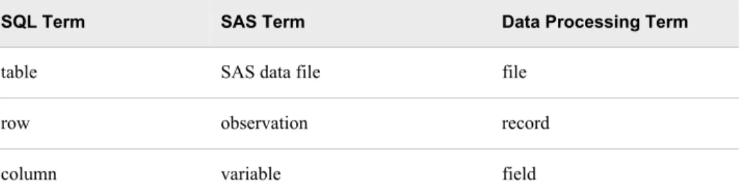
A PROC SQL table is the same as a SAS data file. It is a SAS file of type DATA. PROC SQL tables consist of rows and columns. The rows correspond to observations in SAS data files, and the columns correspond to variables. The following table lists equivalent terms that are used in SQL, SAS, and traditional data processing.

Table 1.1 Comparing Equivalent Terms

SQL Term SAS Term Data Processing Term

table SAS data file file

row observation record

column variable field

You can create and modify tables by using the SAS DATA step, or by using the PROC SQL statements that are described in Chapter 4, “Creating and Updating Tables and Views,” on page 109. Other SAS procedures and the DATA step can read and update tables that are created with PROC SQL.

SAS data files can have a one-level name or a two-level name. Typically, the names of temporary SAS data files have only one level, and the data files are stored in the WORK library. PROC SQL assumes that SAS data files that are specified with a one-level name are to be read from or written to the WORK library, unless you specify a USER library. You can assign a USER library with a LIBNAME statement or with the SAS system option USER=. For more information about how to work with SAS data files and libraries, see “Temporary and Permanent SAS Data Sets” in Chapter 2 of Base SAS Procedures Guide.

DBMS tables are tables that were created with other software vendors' database management systems. PROC SQL can connect to, update, and modify DBMS tables, with some restrictions. For more information, see “Accessing a DBMS with

SAS/ACCESS Software” on page 162.

Queries

Queries retrieve data from a table, view, or DBMS. A query returns a query result, which consists of rows and columns from a table. With PROC SQL, you use a SELECT

(21)

statement and its subordinate clauses to form a query. Chapter 2, “Retrieving Data from a Single Table,” on page 19 describes how to build a query.

Views

PROC SQL views do not actually contain data as tables do. Rather, a PROC SQL view contains a stored SELECT statement or query. The query executes when you use the view in a SAS procedure or DATA step. When a view executes, it displays data that is derived from existing tables, from other views, or from SAS/ACCESS views. Other SAS procedures and the DATA step can use a PROC SQL view as they would any SAS data file. For more information about views, see Chapter 4, “Creating and Updating Tables and Views,” on page 109.

Note: When you process PROC SQL views between a client and a server, getting the correct results depends on the compatibility between the client and server

architecture. For more information, see “Accessing a SAS View” in Chapter 17 of SAS/CONNECT User's Guide.

Null Values

According to the ANSI standard for SQL, a missing value is called a null value. It is not the same as a blank or zero value. However, to be compatible with the rest of SAS, PROC SQL treats missing values the same as blanks or zero values, and considers all three to be null values. This important concept comes up in several places in this document.

Comparing PROC SQL with the SAS DATA Step

PROC SQL can perform some of the operations that are provided by the DATA step and the PRINT, SORT, and SUMMARY procedures. The following query displays the total population of all the large countries (countries with population greater than 1 million) on each continent.

proc sql;

title 'Population of Large Countries Grouped by Continent'; select Continent, sum(Population) as TotPop format=comma15. from sql.countries

where Population gt 1000000 group by Continent

order by TotPop; quit;

(22)

Output 1.1 Sample SQL Output

Here is a SAS program that produces the same result.

title 'Large Countries Grouped by Continent'; proc summary data=sql.countries;

where Population > 1000000; class Continent;

var Population;

output out=sumPop sum=TotPop; run;

proc sort data=SumPop; by totPop;

run;

proc print data=SumPop noobs; var Continent TotPop; format TotPop comma15.; where _type_=1;

(23)

Output 1.2 Sample DATA Step Output

This example shows that PROC SQL can achieve the same results as Base SAS software but often with fewer and shorter statements. The SELECT statement that is shown in this example performs summation, grouping, sorting, and row selection. It also displays the query's results without the PRINT procedure.

PROC SQL executes without using the RUN statement. After you invoke PROC SQL you can submit additional SQL procedure statements without submitting the PROC statement again. Use the QUIT statement to terminate the procedure.

Notes about the Example Tables

For all examples, the following global statement is in effect:

libname sql 'SAS-data-library';

The tables that are used in this document contain geographic and demographic data. The data is intended to be used for the PROC SQL code examples only; it is not necessarily up-to-date or accurate.

Note: You can find instructions for downloading these data sets at http://

ftp.sas.com/samples/A56936. These data sets are valid for SAS 9 as well as previous versions of SAS.

(24)

The COUNTRIES table contains data that pertains to countries. The Area column contains a country's area in square miles. The UNDate column contains the year a country entered the United Nations, if applicable.

Output 1.3 COUNTRIES (Partial Output)

The WORLDCITYCOORDS table contains latitude and longitude data for world cities. Cities in the Western hemisphere have negative longitude coordinates. Cities in the

(25)

Southern hemisphere have negative latitude coordinates. Coordinates are rounded to the nearest degree.

Output 1.4 WORLDCITYCOORDS (Partial Output)

(26)

The USCITYCOORDS table contains the coordinates for cities in the United States. Because all cities in this table are in the Western hemisphere, all of the longitude coordinates are negative. Coordinates are rounded to the nearest degree.

(27)

The UNITEDSTATES table contains data that is associated with the states. The Statehood column contains the date when the state was admitted into the Union. Output 1.6 UNITEDSTATES (Partial Output)

(28)

The POSTALCODES table contains postal code abbreviations. Output 1.7 POSTALCODES (Partial Output)

(29)

The WORLDTEMPS table contains average high and low temperatures from various international cities.

Output 1.8 WORLDTEMPS (Partial Output)

(30)

The OILPROD table contains oil production statistics from oil-producing countries. Output 1.9 OILPROD (Partial Output)

(31)

The OILRSRVS table lists approximate oil reserves of oil-producing countries. Output 1.10 OILRSRVS (Partial Output)

(32)

The CONTINENTS table contains geographic data that relates to world continents. Output 1.11 CONTINENTS

(33)

The FEATURES table contains statistics that describe various types of geographical features, such as oceans, lakes, and mountains.

Output 1.12 FEATURES (Partial Output)

(34)

(35)

Chapter 2

Retrieving Data from a Single

Table

Overview of the SELECT Statement . . . 20

How to Use the SELECT Statement . . . 20

SELECT and FROM Clauses . . . 20

WHERE Clause . . . 21

ORDER BY Clause . . . 21

GROUP BY Clause . . . 21

HAVING Clause . . . 21

Ordering the SELECT Statement . . . 22

Selecting Columns in a Table . . . 22

Selecting All Columns in a Table . . . 22

Selecting Specific Columns in a Table . . . 23

Eliminating Duplicate Rows from the Query Results . . . 25

Determining the Structure of a Table . . . 27

Creating New Columns . . . 27

Adding Text to Output . . . 27

Calculating Values . . . 29

Assigning a Column Alias . . . 30

Referring to a Calculated Column by Alias . . . 31

Assigning Values Conditionally . . . 32

Replacing Missing Values . . . 35

Specifying Column Attributes . . . 36

Sorting Data . . . 37

Overview of Sorting Data . . . 37

Sorting by Column . . . 38

Sorting by Multiple Columns . . . 38

Specifying a Sort Order . . . 39

Sorting by Calculated Column . . . 40

Sorting by Column Position . . . 41

Sorting by Columns That Are Not Selected . . . 42

Specifying a Different Sorting Sequence . . . 43

Sorting Columns That Contain Missing Values . . . 43

Retrieving Rows That Satisfy a Condition . . . 44

Using a Simple WHERE Clause . . . 44

Retrieving Rows Based on a Comparison . . . 45

Retrieving Rows That Satisfy Multiple Conditions . . . 47

Using Other Conditional Operators . . . 49

Using Truncated String Comparison Operators . . . 53

Using a WHERE Clause with Missing Values . . . 54

Summarizing Data . . . 56

(36)

Overview of Summarizing Data . . . 56

Using Aggregate Functions . . . 56

Summarizing Data with a WHERE Clause . . . 57

Displaying Sums . . . 58

Combining Data from Multiple Rows into a Single Row . . . 59

Remerging Summary Statistics . . . 59

Using Aggregate Functions with Unique Values . . . 61

Summarizing Data with Missing Values . . . 62

Grouping Data . . . 64

Grouping by One Column . . . 64

Grouping without Summarizing . . . 64

Grouping by Multiple Columns . . . 65

Grouping and Sorting Data . . . 66

Grouping with Missing Values . . . 67

Filtering Grouped Data . . . 69

Overview of Filtering Grouped Data . . . 69

Using a Simple HAVING Clause . . . 69

Choosing between HAVING and WHERE . . . 70

Using HAVING with Aggregate Functions . . . 70

Validating a Query . . . 71

Overview of the SELECT Statement

How to Use the SELECT Statement

This chapter shows you how to perform the following tasks: • retrieve data from a single table by using the SELECT statement

• validate the correctness of a SELECT statement by using the VALIDATE statement With the SELECT statement, you can retrieve data from tables or data that is described by SAS data views.

Note: The examples in this chapter retrieve data from tables that are SAS data sets. However, you can use all of the operations that are described here with SAS data views.

The SELECT statement is the primary tool of PROC SQL. You use it to identify, retrieve, and manipulate columns of data from a table. You can also use several optional clauses within the SELECT statement to place restrictions on a query.

SELECT and FROM Clauses

The following simple SELECT statement is sufficient to produce a useful result:

select Name

from sql.countries;

The SELECT statement must contain a SELECT clause and a FROM clause, both of which are required in a PROC SQL query. This SELECT statement contains the following:

(37)

• a FROM clause that lists the table in which the Name column resides

WHERE Clause

The WHERE clause enables you to restrict the data that you retrieve by specifying a condition that each row of the table must satisfy. PROC SQL output includes only those rows that satisfy the condition. The following SELECT statement contains a WHERE clause that restricts the query output to only those countries that have a population that is greater than 5,000,000 people:

select Name

from sql.countries

where Population gt 5000000;

ORDER BY Clause

The ORDER BY clause enables you to sort the output from a table by one or more columns. That is, you can put character values in either ascending or descending alphabetical order, and you can put numerical values in either ascending or descending numerical order. The default order is ascending. For example, you can modify the previous example to list the data by descending population:

select Name

from sql.countries

where Population gt 5000000 order by Population desc;

GROUP BY Clause

The GROUP BY clause enables you to break query results into subsets of rows. When you use the GROUP BY clause, you use an aggregate function in the SELECT clause or a HAVING clause to instruct PROC SQL how to group the data. For details about aggregate functions, see “Summarizing Data” on page 56. PROC SQL calculates the aggregate function separately for each group. When you do not use an aggregate function, PROC SQL treats the GROUP BY clause as if it were an ORDER BY clause, and any aggregate functions are applied to the entire table.

The following query uses the SUM function to list the total population of each continent. The GROUP BY clause groups the countries by continent, and the ORDER BY clause puts the continents in alphabetical order:

select Continent, sum(Population) from sql.countries

group by Continent order by Continent;

HAVING Clause

The HAVING clause works with the GROUP BY clause to restrict the groups in a query's results based on a given condition. PROC SQL applies the HAVING condition after grouping the data and applying aggregate functions. For example, the following query restricts the groups to include only the continents of Asia and Europe:

(38)

select Continent, sum(Population) from sql.countries

group by Continent

having Continent in ('Asia', 'Europe') order by Continent;

Ordering the SELECT Statement

When you construct a SELECT statement, you must specify the clauses in the following order: 1. SELECT 2. FROM 3. WHERE 4. GROUP BY 5. HAVING 6. ORDER BY

Note: Only the SELECT and FROM clauses are required.

The PROC SQL SELECT statement and its clauses are discussed in further detail in the following sections.

Selecting Columns in a Table

When you retrieve data from a table, you can select one or more columns by using variations of the basic SELECT statement.

Selecting All Columns in a Table

Use an asterisk in the SELECT clause to select all columns in a table. The following example selects all columns in the SQL.USCITYCOORDS table, which contains latitude and longitude values for U.S. cities:

libname sql 'SAS-library'; proc sql outobs=12;

title 'U.S. Cities with Their States and Coordinates'; select *

from sql.uscitycoords;

Note: The OUTOBS= option limits the number of rows (observations) in the output. OUTOBS= is similar to the OBS= data set option. OUTOBS= is used throughout this document to limit the number of rows that are displayed in examples.

Note: In the tables used in these examples, latitude values that are south of the Equator are negative. Longitude values that are west of the Prime Meridian are also negative.

(39)

Output 2.1 Selecting All Columns in a Table

Note: When you select all columns, PROC SQL displays the columns in the order in which they are stored in the table.

Selecting Specific Columns in a Table

To select a specific column in a table, list the name of the column in the SELECT clause. The following example selects only the City column in the SQL.USCITYCOORDS table:

title 'Names of U.S. Cities'; select City

from sql.uscitycoords;

(40)

Output 2.2 Selecting One Column

If you want to select more than one column, then you must separate the names of the columns with commas, as in this example, which selects the City and State columns in the SQL.USCITYCOORDS table:

title 'U.S. Cities and Their States'; select City, State

(41)

Output 2.3 Selecting Multiple Columns

Note: When you select specific columns, PROC SQL displays the columns in the order in which you specify them in the SELECT clause.

Eliminating Duplicate Rows from the Query Results

In some cases, you might want to find only the unique values in a column. For example, if you want to find the unique continents in which U.S. states are located, then you might begin by constructing the following query:

title 'Continents of the United States'; select Continent

from sql.unitedstates;

(42)

Output 2.4 Selecting a Column with Duplicate Values

You can eliminate the duplicate rows from the results by using the DISTINCT keyword in the SELECT clause. Compare the previous example with the following query, which uses the DISTINCT keyword to produce a single row of output for each continent that is in the SQL.UNITEDSTATES table:

libname sql 'SAS-library'; proc sql;

title 'Continents of the United States'; select distinct Continent

from sql.unitedstates;

Output 2.5 Eliminating Duplicate Values

Note: When you specify all of a table's columns in a SELECT clause with the DISTINCT keyword, PROC SQL eliminates duplicate rows, or rows in which the values in all of the columns match, from the results.

(43)

Determining the Structure of a Table

To obtain a list of all of the columns in a table and their attributes, you can use the DESCRIBE TABLE statement. The following example generates a description of the SQL.UNITEDSTATES table. PROC SQL writes the description to the log.

describe table sql.unitedstates;

Log 2.1 Determining the Structure of a Table (Partial Log)

NOTE: SQL table SQL.UNITEDSTATES was created like: create table SQL.UNITEDSTATES( bufsize=12288 ) (

Name char(35) format=$35. informat=$35. label='Name', Capital char(35) format=$35. informat=$35. label='Capital', Population num format=BEST8. informat=BEST8. label='Population', Area num format=BEST8. informat=BEST8.,

Continent char(35) format=$35. informat=$35. label='Continent', Statehood num

);

Creating New Columns

In addition to selecting columns that are stored in a table, you can create new columns that exist for the duration of the query. These columns can contain text or calculations. PROC SQL writes the columns that you create as if they were columns from the table.

Adding Text to Output

You can add text to the output by including a string expression, or literal expression, in a query. The following query includes two strings as additional columns in the output:

title 'U.S. Postal Codes';

select 'Postal code for', Name, 'is', Code from sql.postalcodes;

(44)

Output 2.6 Adding Text to Output

To prevent the column headings Name and Code from printing, you can assign a label that starts with a special character to each of the columns. PROC SQL does not output the column name when a label is assigned, and it does not output labels that begin with special characters. For example, you could use the following query to suppress the column headings that PROC SQL displayed in the previous example:

title 'U.S. Postal Codes';

select 'Postal code for', Name label='#', 'is', Code label='#' from sql.postalcodes;

(45)

Output 2.7 Suppressing Column Headings in Output

Calculating Values

You can perform calculations with values that you retrieve from numeric columns. The following example converts temperatures in the SQL.WORLDTEMPS table from Fahrenheit to Celsius:

title 'Low Temperatures in Celsius'; select City, (AvgLow - 32) * 5/9 format=4.1 from sql.worldtemps;

Note: This example uses the FORMAT attribute to modify the format of the calculated output. For more information, see “Specifying Column Attributes” on page 36.

(46)

Output 2.8 Calculating Values

Assigning a Column Alias

By specifying a column alias, you can assign a new name to any column within a PROC SQL query. The new name must follow the rules for SAS names. The name persists only for that query.

When you use an alias to name a column, you can use the alias to reference the column later in the query. PROC SQL uses the alias as the column heading in output. The following example assigns an alias of LowCelsius to the calculated column from the previous example:

title 'Low Temperatures in Celsius';

select City, (AvgLow - 32) * 5/9 as LowCelsius format=4.1 from sql.worldtemps;

(47)

Output 2.9 Assigning a Column Alias to a Calculated Column

Referring to a Calculated Column by Alias

When you use a column alias to refer to a calculated value, you must use the CALCULATED keyword with the alias to inform PROC SQL that the value is calculated within the query. The following example uses two calculated values, LowC and HighC, to calculate a third value, Range:

title 'Range of High and Low Temperatures in Celsius'; select City, (AvgHigh - 32) * 5/9 as HighC format=5.1, (AvgLow - 32) * 5/9 as LowC format=5.1, (calculated HighC - calculated LowC) as Range format=4.1

from sql.worldtemps;

Note: You can use an alias to refer to a calculated column in a SELECT clause, a WHERE clause, or ORDER BY clause.

(48)

Output 2.10 Referring to a Calculated Column by Alias

Note: Because this query sets a numeric format of 4.1 on the HighC, LowC, and Range columns, the values in those columns are rounded to the nearest tenth. As a result of the rounding, some of the values in the HighC and LowC columns do not reflect the range value output for the Range column. When you round numeric data values, this type of error sometimes occurs. If you want to avoid this problem, then you can specify additional decimal places in the format.

Assigning Values Conditionally

Using a Simple CASE Expression

CASE expressions enable you to interpret and change some or all of the data values in a column to make the data more useful or meaningful.

You can use conditional logic within a query by using a CASE expression to

conditionally assign a value. You can use a CASE expression anywhere that you can use a column name.

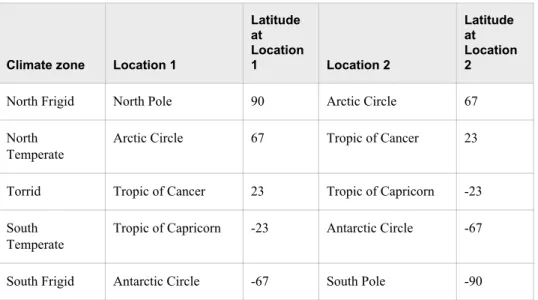
The following table, which is used in the next example, describes the world climate zones (rounded to the nearest degree) that exist between Location 1 and Location 2:

(49)

Table 2.1 World Climate Zones

Climate zone Location 1

Latitude at Location 1 Location 2 Latitude at Location 2

North Frigid North Pole 90 Arctic Circle 67

North Temperate

Arctic Circle 67 Tropic of Cancer 23

Torrid Tropic of Cancer 23 Tropic of Capricorn -23

South Temperate

Tropic of Capricorn -23 Antarctic Circle -67

South Frigid Antarctic Circle -67 South Pole -90

In this example, a CASE expression determines the climate zone for each city based on the value in the Latitude column in the SQL.WORLDCITYCOORDS table. The query also assigns an alias of ClimateZone to the value. You must close the CASE logic with the END keyword.

title 'Climate Zones of World Cities'; select City, Country, Latitude, case

when Latitude gt 67 then 'North Frigid'

when 67 ge Latitude ge 23 then 'North Temperate' when 23 gt Latitude gt -23 then 'Torrid'

when -23 ge Latitude ge -67 then 'South Temperate' else 'South Frigid'

end as ClimateZone from sql.worldcitycoords order by City;

(50)

Output 2.11 Using a Simple CASE Expression

Using the CASE-OPERAND Form

You can also construct a CASE expression by using the CASE-OPERAND form, as in the following example. This example selects states and assigns them to a region based on the value of the Continent column:

title 'Assigning Regions to Continents'; select Name, Continent,

case Continent

when 'North America' then 'Continental U.S.' when 'Oceania' then 'Pacific Islands' else 'None'

end as Region from sql.unitedstates;

Note: When you use the CASE-OPERAND form of the CASE expression, the conditions must all be equality tests. That is, they cannot use comparison operators or other types of operators, as are used in “Using a Simple CASE Expression” on page 32.

(51)

Output 2.12 Using a CASE Expression in the CASE-OPERAND Form

Replacing Missing Values

The COALESCE function enables you to replace missing values in a column with a new value that you specify. For every row that the query processes, the COALESCE function checks each of its arguments until it finds a nonmissing value, and then returns that value. If all of the arguments are missing values, then the COALESCE function returns a missing value. For example, the following query replaces missing values in the

LowPoint column in the SQL.CONTINENTS table with the words Not Available:

title 'Continental Low Points';

select Name, coalesce(LowPoint, 'Not Available') as LowPoint from sql.continents;

(52)

Output 2.13 Using the COALESCE Function to Replace Missing Values

The following CASE expression shows another way to perform the same replacement of missing values. However, the COALESCE function requires fewer lines of code to obtain the same results:

title 'Continental Low Points'; select Name, case

when LowPoint is missing then 'Not Available' else Lowpoint

end as LowPoint from sql.continents;

Specifying Column Attributes

You can specify the following column attributes, which determine how SAS data is displayed:

• FORMAT= • INFORMAT= • LABEL= • LENGTH=

If you do not specify these attributes, then PROC SQL uses attributes that are already saved in the table or, if no attributes are saved, then it uses the default attributes. The following example assigns a label of State to the Name column and a format of COMMA10. to the Area column:

(53)

title 'Areas of U.S. States in Square Miles'; select Name label='State', Area format=comma10. from sql.unitedstates;

Note: Using the LABEL= keyword is optional. For example, the following two select clauses are the same:

select Name label='State', Area format=comma10. select Name 'State', Area format=comma10.

Output 2.14 Specifying Column Attributes

Sorting Data

Overview of Sorting Data

You can sort query results with an ORDER BY clause by specifying any of the columns in the table, including columns that are not selected or columns that are calculated. Unless an ORDER BY clause is included in the SELECT statement, then a particular order to the output rows, such as the order in which the rows are encountered in the queried table, cannot be guaranteed, even if an index is present. Without an ORDER BY clause, the order of the output rows is determined by the internal processing of PROC SQL, the default collating sequence of SAS, and your operating environment. Therefore, if you want your result table to appear in a particular order, then use the ORDER BY clause.

(54)

For more information and examples, see the “ORDER BY Clause” on page 303.

Sorting by Column

The following example selects countries and their populations from the SQL.COUNTRIES table and orders the results by population:

title 'Country Populations';

select Name, Population format=comma10. from sql.countries

order by Population;

Note: When you use an ORDER BY clause, you change the order of the output but not the order of the rows that are stored in the table.

Note: The PROC SQL default sort order is ascending.

Output 2.15 Sorting by Column

Sorting by Multiple Columns

You can sort by more than one column by specifying the column names, separated by commas, in the ORDER BY clause. The following example sorts the SQL.COUNTRIES table by two columns, Continent and Name:

(55)

proc sql outobs=12;

title 'Countries, Sorted by Continent and Name'; select Name, Continent

from sql.countries order by Continent, Name;

Output 2.16 Sorting by Multiple Columns

Note: The results list countries without continents first because PROC SQL sorts missing values first in an ascending sort.

Specifying a Sort Order

To order the results, specify ASC for ascending or DESC for descending. You can specify a sort order for each column in the ORDER BY clause.

When you specify multiple columns in the ORDER BY clause, the first column

determines the primary row order of the results. Subsequent columns determine the order of rows that have the same value for the primary sort. The following example sorts the SQL.FEATURES table by feature type and name:

title 'World Topographical Features'; select Name, Type

from sql.features

order by Type desc, Name;

(56)

Note: The ASC keyword is optional because the PROC SQL default sort order is ascending.

Output 2.17 Specifying a Sort Order

Sorting by Calculated Column

You can sort by a calculated column by specifying its alias in the ORDER BY clause. The following example calculates population densities and then performs a sort on the calculated Density column:

title 'World Population Densities per Square Mile';

select Name, Population format=comma12., Area format=comma8., Population/Area as Density format=comma10.

from sql.countries order by Density desc;

(57)

Output 2.18 Sorting by Calculated Column

Sorting by Column Position

You can sort by any column within the SELECT clause by specifying its numerical position. By specifying a position instead of a name, you can sort by a calculated column that has no alias. The following example does not assign an alias to the calculated density column. Instead, the column position of 4 in the ORDER BY clause refers to the position of the calculated column in the SELECT clause:

title 'World Population Densities per Square Mile';

select Name, Population format=comma12., Area format=comma8., Population/Area format=comma10. label='Density' from sql.countries

order by 4 desc;

Note: PROC SQL uses a label, if one has been assigned, as a heading for a column that does not have an alias.

(58)

Output 2.19 Sorting by Column Position

Sorting by Columns That Are Not Selected

You can sort query results by columns that are not included in the query. For example, the following query returns all the rows in the SQL.COUNTRIES table and sorts them by population, even though the Population column is not included in the query:

title 'Countries, Sorted by Population'; select Name, Continent

from sql.countries order by Population;

(59)

Output 2.20 Sorting by Columns That Are Not Selected

Specifying a Different Sorting Sequence

SORTSEQ= is a PROC SQL statement option that specifies the sorting sequence for PROC SQL to use when a query contains an ORDER BY clause. Use this option only if you want to use a sorting sequence other than your operating environment's default sorting sequence. Possible values include ASCII, EBCDIC, and some languages other than English. For example, in an operating environment that supports the EBCDIC sorting sequence, you could use the following option in the PROC SQL statement to set the sorting sequence to EBCDIC:

proc sql sortseq=ebcdic;

Note: SORTSEQ= affects only the ORDER BY clause. It does not override your operating environment's default comparison operations for the WHERE clause. Operating Environment Information

See the SAS documentation for your operating environment for more information about the default and other sorting sequences for your operating environment.

Sorting Columns That Contain Missing Values

PROC SQL sorts nulls, or missing values, before character or numeric data. Therefore, when you specify ascending order, missing values appear first in the query results. The following example sorts the rows in the CONTINENTS table by the LowPoint column:

(60)

title 'Continents, Sorted by Low Point'; select Name, LowPoint

from sql.continents order by LowPoint;

Because three continents have a missing value in the LowPoint column, those continents appear first in the output. Note that because the query does not specify a secondary sort, rows that have the same value in the LowPoint column, such as the first three rows of output, are not displayed in any particular order. In general, if you do not explicitly specify a sort order, then PROC SQL output is not guaranteed to be in any particular order.

Output 2.21 Sorting Columns That Contain Missing Values

Retrieving Rows That Satisfy a Condition

The WHERE clause enables you to retrieve only rows from a table that satisfy a

condition. WHERE clauses can contain any of the columns in a table, including columns that are not selected.

Using a Simple WHERE Clause

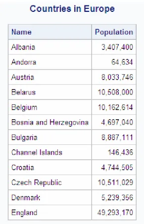
The following example uses a WHERE clause to find all countries that are in the continent of Europe and their populations:

title 'Countries in Europe';

(61)

from sql.countries

where Continent = 'Europe';

Output 2.22 Using a Simple WHERE Clause

Retrieving Rows Based on a Comparison

You can use comparison operators in a WHERE clause to select different subsets of data. The following table lists the comparison operators that you can use:

Table 2.2 Comparison Operators

Symbol

Mnemonic

Equivalent Definition Example

= EQ equal to where Name =

'Asia';

^= or ~= or ¬= or <> NE not equal to where Name ne 'Africa';

> GT greater than where Area >

10000;

< LT less than where Depth <

5000;

(62)

Symbol

Mnemonic

>= GE greater than or equal

to whereStatehood >= '01jan1860'd;

<= LE less than or equal to where

Population <= 5000000;

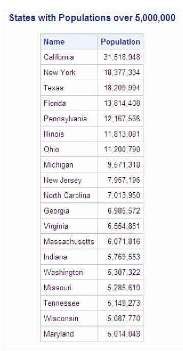
The following example subsets the SQL.UNITEDSTATES table by including only states with populations greater than 5,000,000 people:

title 'States with Populations over 5,000,000'; select Name, Population format=comma10.

from sql.unitedstates where Population gt 5000000 order by Population desc;

(63)

Output 2.23 Retrieving Rows Based on a Comparison

Retrieving Rows That Satisfy Multiple Conditions

You can use logical, or Boolean, operators to construct a WHERE clause that contains two or more expressions. The following table lists the logical operators that you can use: Table 2.3 Logical (Boolean) Operators

Symbol

Mnemonic

& AND specifies that both the

previous and following conditions must be true

Continent = 'Asia' and Population > 5000000

(64)

Symbol

Mnemonic

! or | or ¦ OR specifies that either the

previous or the following condition must be true Population < 1000000 or Population > 5000000

^ or ~ or ¬ NOT specifies that the

following condition must be false

Continent not 'Africa'

The following example uses two expressions to include only countries that are in Africa and that have a population greater than 20,000,000 people:

title 'Countries in Africa with Populations over 20,000,000'; select Name, Population format=comma10.

from sql.countries

where Continent = 'Africa' and Population gt 20000000 order by Population desc;

Output 2.24 Retrieving Rows That Satisfy Multiple Conditions

Note: You can use parentheses to improve the readability of WHERE clauses that contain multiple, or compound, expressions, such as the following:

where (Continent = 'Africa' and Population gt 2000000) or (Continent = 'Asia' and Population gt 1000000)

(65)

Using Other Conditional Operators

Overview of Using Other Conditional Operators

You can use many different conditional operators in a WHERE clause. The following table lists other operators that you can use:

Table 2.4 Conditional Operators

Operator Definition Example

ANY specifies that at least one

of a set of values obtained from a subquery must satisfy a given condition

where Population > any (select Population from sql.countries)

ALL specifies that all of the

values obtained from a subquery must satisfy a given condition

where Population > all (select Population from sql.countries)

BETWEEN-AND tests for values within an

inclusive range where Population between1000000 and 5000000 CONTAINS tests for values that

contain a specified string where Continent contains_'America'; EXISTS tests for the existence of

a set of values obtained from a subquery

where exists (select * from sql.oilprod);

IN tests for values that

match one of a list of values

where Name in ('Africa', 'Asia');

IS NULL or IS MISSING tests for missing values where Population is missing;

LIKE tests for values that

match a specified pattern1

where Continent like 'A %';

=* tests for values that

sound like a specified value

where Name =* 'Tiland';

Note: All of these operators can be prefixed with the NOT operator to form a negative condition.

1 You can use a percent symbol (%) to match any number of characters. You can use an underscore (_) to match one arbitrary character.

(66)

Using the IN Operator

The IN operator enables you to include values within a list that you supply. The following example uses the IN operator to include only the mountains and waterfalls in the SQL.FEATURES table:

title 'World Mountains and Waterfalls'; select Name, Type, Height format=comma10. from sql.features

where Type in ('Mountain', 'Waterfall') order by Height;

Output 2.25 Using the IN Operator

Using the IS MISSING Operator

The IS MISSING operator enables you to identify rows that contain columns with missing values. The following example selects countries that are not located on a continent. That is, these countries have a missing value in the Continent column:

proc sql;

title 'Countries with Missing Continents'; select Name, Continent

from sql.countries

where Continent is missing;

Note: The IS NULL operator is the same as, and interchangeable with, the IS MISSING operator.

(67)

Output 2.26 Using the IS MISSING Operator

Using the BETWEEN-AND Operators

To select rows based on a range of values, you can use the BETWEEN-AND operators. This example selects countries that have latitudes within five degrees of the Equator:

proc sql outobs=12;

title 'Equatorial Cities of the World'; select City, Country, Latitude

from sql.worldcitycoords

where Latitude between -5 and 5;

Note: In the tables used in these examples, latitude values that are south of the Equator are negative. Longitude values that are west of the Prime Meridian are also negative. Note: Because the BETWEEN-AND operators are inclusive, the values that you specify

in the BETWEEN-AND expression are included in the results.

(68)

Output 2.27 Using the BETWEEN-AND Operators

Using the LIKE Operator

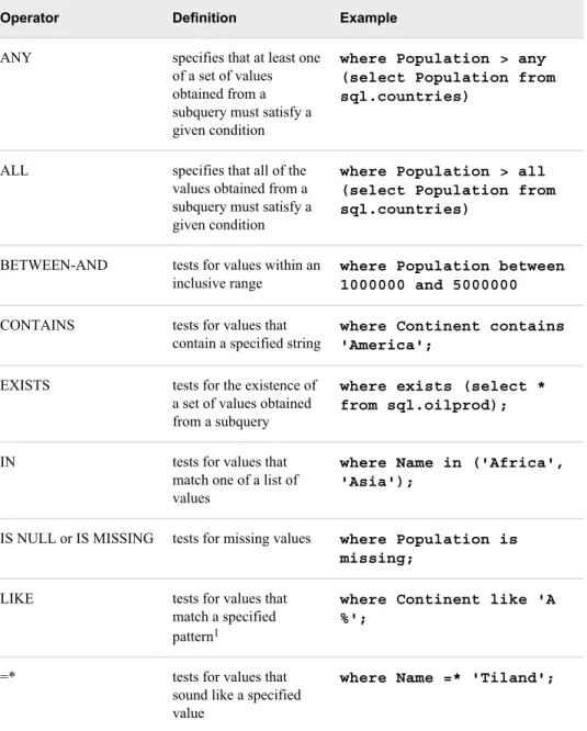
The LIKE operator enables you to select rows based on pattern matching. For example, the following query returns all countries in the SQL.COUNTRIES table that begin with the letter Z and are any number of characters long, or end with the letter a and are five characters long:

title1 'Country Names that Begin with the Letter "Z"';

title2 'or Are 5 Characters Long and End with the Letter "a"'; select Name

from sql.countries

(69)

Output 2.28 Using the LIKE Operator

The percent sign (%) and underscore (_) are wildcard characters. For more information about pattern matching with the LIKE comparison operator, see Chapter 7, “SQL Procedure,” on page 209.

Using Truncated String Comparison Operators

Truncated string comparison operators are used to compare two strings. They differ from conventional comparison operators in that, before executing the comparison, PROC SQL truncates the longer string to be the same length as the shorter string. The truncation is performed internally; neither operand is permanently changed. The following table lists the truncated comparison operators:

Table 2.5 Truncated String Comparison Operators

Symbol Definition Example

EQT equal to truncated strings where Name eqt 'Aust';

GTT greater than truncated strings where Name gtt 'Bah';

LTT less than truncated strings where Name ltt 'An';

GET greater than or equal to truncated strings where Country get 'United A';

LET less than or equal to truncated strings where Lastname let 'Smith';

(70)

Symbol Definition Example

NET not equal to truncated strings where Style net 'TWO';

The following example returns a list of U.S. states that have 'New ' at the beginning of their names:

proc sql;

title '"New" U.S. States'; select Name

from sql.unitedstates where Name eqt 'New ';

Output 2.29 Using a Truncated String Comparison Operator

Using a WHERE Clause with Missing Values

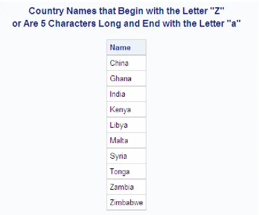
If a column that you specify in a WHERE clause contains missing values, then a query might provide unexpected results. For example, the following query returns all features from the SQL.FEATURES table that have a depth of less than 500 feet:

libname sql 'SAS-library'; /* incorrect output */ proc sql outobs=12;

title 'World Features with a Depth of Less than 500 Feet'; select Name, Depth

from sql.features where Depth lt 500 order by Depth;

(71)

Output 2.30 Using a WHERE Clause with Missing Values (Incorrect Output)

However, because PROC SQL treats missing values as smaller than nonmissing values, features that have no depth listed are also included in the results. To avoid this problem, you could adjust the WHERE expression to check for missing values and exclude them from the query results, as follows:

libname sql 'SAS-library'; /* corrected output */ proc sql outobs=12;

title 'World Features with a Depth of Less than 500 Feet'; select Name, Depth

from sql.features

where Depth lt 500 and Depth is not missing order by Depth;

(72)

Output 2.31 Using a WHERE Clause with Missing Values (Corrected Output)

Summarizing Data

Overview of Summarizing Data

You can use an aggregate function (or summary function) to produce a statistical summary of data in a table. The aggregate function instructs PROC SQL in how to combine data in one or more columns. If you specify one column as the argument to an aggregate function, then the values in that column are calculated. If you specify multiple arguments, then the arguments or columns that are listed are calculated.

Note: When more than one argument is used within an SQL aggregate function, the function is no longer considered to be an SQL aggregate or summary function. If there is a like-named Base SAS function, then PROC SQL executes the Base SAS function and the results that are returned are based on the values for the current row. If no like-named Base SAS function exists, then an error will occur. For example, if you use multiple arguments for the AVG function, an error will occur because there is no AVG function for Base SAS.

When you use an aggregate function, PROC SQL applies the function to the entire table, unless you use a GROUP BY clause. You can use aggregate functions in the SELECT or HAVING clauses.

Note: See “Grouping Data” on page 64 for information about producing summaries of individual groups of data within a table.

Using Aggregate Functions

The following table lists the aggregate functions that you can use: Table 2.6 Aggregate Functions

Function Definition

AVG, MEAN mean or average of values

(73)

Function Definition

CSS corrected sum of squares

CV coefficient of variation (percent)

MAX largest value

MIN smallest value

NMISS number of missing values

PRT probability of a greater absolute value of

Student's t

RANGE range of values

STD standard deviation

STDERR standard error of the mean

SUM sum of values

SUMWGT sum of the WEIGHT variable values1

T Student's t value for testing the hypothesis

that the population mean is zero

USS uncorrected sum of squares

VAR variance

Note: You can use most other SAS functions in PROC SQL, but they are not treated as aggregate functions.

Summarizing Data with a WHERE Clause

Overview of Summarizing Data with a WHERE Clause

You can use aggregate, or summary functions, by using a WHERE clause. For a complete list of the aggregate functions that you can use, see Table 2.6 on page 56.

Using the MEAN Function with a WHERE Clause

This example uses the MEAN function to find the annual mean temperature for each country in the SQL.WORLDTEMPS table. The WHERE clause returns countries with a mean temperature that is greater than 75 degrees.

title 'Mean Temperatures for World Cities';

1 In the SQL procedure, each row has a weight of 1.

(74)

select City, Country, mean(AvgHigh, AvgLow) as MeanTemp

from sql.worldtemps

where calculated MeanTemp gt 75 order by MeanTemp desc;

Note: You must use the CALCULATED keyword to reference the calculated column.

Output 2.32 Using the MEAN Function with a WHERE Clause

Displaying Sums

The following example uses the SUM function to return the total oil reserves for all countries in the SQL.OILRSRVS table:

title 'World Oil Reserves';

select sum(Barrels) format=comma18. as TotalBarrels from sql.oilrsrvs;

Note: The SUM function produces a single row of output for the requested sum because no nonaggregate value appears in the SELECT clause.

(75)

Output 2.33 Displaying Sums

Combining Data from Multiple Rows into a Single Row

In the previous example, PROC SQL combined information from multiple rows of data into a single row of output. Specifically, the world oil reserves for each country were combined to form a total for all countries. Combining, or rolling up, of rows occurs when the following conditions exist:

• The SELECT clause contains only columns that are specified within an aggregate function.

• The WHERE clause, if there is one, contains only columns that are specified in the SELECT clause.

Remerging Summary Statistics

The following example uses the MAX function to find the largest population in the SQL.COUNTRIES table and displays it in a column called MaxPopulation. Aggregate functions, such as the MAX function, can cause the same calculation to repeat for every row. This occurs whenever PROC SQL remerges data. Remerging occurs whenever any of the following conditions exist:

• The SELECT clause references a column that contains an aggregate function that is not listed in a GROUP BY clause.

• The SELECT clause references a column that contains an aggregate function and other c

SAS 9.3 SQL Procedure

9.3 SQL Procedure

SAS® 9.3 SQL Procedure User’s Guide

For a Web download or e-book:Your use of this publication shall be governed by the terms established by the vendor at the time you acquire this

Contents

Chapter 2 • Retrieving Data from a Single Table . . . 19

Chapter 4 • Creating and Updating Tables and Views . . . 109

Chapter 5 • Programming with the SQL Procedure . . . 135

Chapter 6 • Practical Problem-Solving with PROC SQL . . . 171

SQL Procedure Reference

Chapter 8 • SQL SELECT Statement Clauses . . . 291

Appendixes

Appendix 2 • PROC SQL and the ANSI Standard . . . 373

About This Book

Overview of Syntax Conventions for the SAS Language

CHAR (string, position) CALL RANBIN (seed, n, p, x); ALTER (alter-password) BEST w.

CHAR (string, position)

Style Conventions

CMPMODEL = BOTH | CATALOG | XML

Special Characters

CMPMODEL = BOTH | CATALOG | XML ...

References to SAS Libraries and External Files

What’s New in the SAS 9.3 SQL

Ability to Optimize the PUT Function

• REDUCEPUTOBS= • REDUCEPUTVALUES= • SQLREDUCEPUTOBS= • SQLREDUCEPUTVALUES=

Ability to Reuse the LIBNAME Statement

• STOPONTRUNC

Additional Macro Variable Specifications for the

Additional System Macro Variable

SQLGENERATION= Option

Recommended Reading

Using the SQL Procedure

Chapter 1

What Is SQL? . . . 3

What Is SQL?

Terminology

Tables

Queries

Null Values

Comparing PROC SQL with the SAS DATA Step

Output 1.1 Sample SQL Output

Output 1.2 Sample DATA Step Output

Notes about the Example Tables

Output 1.3 COUNTRIES (Partial Output)

Output 1.8 WORLDTEMPS (Partial Output)

Output 1.12 FEATURES (Partial Output)

Chapter 2

Overview of the SELECT Statement . . . 20

Creating New Columns . . . 27

Retrieving Rows That Satisfy a Condition . . . 44

Grouping Data . . . 64

Validating a Query . . . 71

Overview of the SELECT Statement

How to Use the SELECT Statement

SELECT and FROM Clauses

WHERE Clause

ORDER BY Clause

GROUP BY Clause

HAVING Clause

Ordering the SELECT Statement

Selecting Columns in a Table

Selecting All Columns in a Table

Output 2.1 Selecting All Columns in a Table

Output 2.2 Selecting One Column

Eliminating Duplicate Rows from the Query Results

Output 2.4 Selecting a Column with Duplicate Values

Output 2.5 Eliminating Duplicate Values

Log 2.1 Determining the Structure of a Table (Partial Log)

Creating New Columns

Adding Text to Output

Output 2.6 Adding Text to Output

Output 2.7 Suppressing Column Headings in Output

Output 2.8 Calculating Values

Output 2.9 Assigning a Column Alias to a Calculated Column

Output 2.10 Referring to a Calculated Column by Alias

Table 2.1 World Climate Zones

Output 2.11 Using a Simple CASE Expression

Output 2.12 Using a CASE Expression in the CASE-OPERAND Form

Output 2.13 Using the COALESCE Function to Replace Missing Values

Specifying Column Attributes