DigitalCommons@USU
DigitalCommons@USU
All Graduate Theses and Dissertations Graduate Studies
5-2017
Vision-Based Control of a Full-Size Car by Lane Detection
Vision-Based Control of a Full-Size Car by Lane Detection
N. Chase KunzUtah State University
Follow this and additional works at: https://digitalcommons.usu.edu/etd
Part of the Electrical and Computer Engineering Commons
Recommended Citation Recommended Citation
Kunz, N. Chase, "Vision-Based Control of a Full-Size Car by Lane Detection" (2017). All Graduate Theses and Dissertations. 6534.
https://digitalcommons.usu.edu/etd/6534
This Thesis is brought to you for free and open access by the Graduate Studies at DigitalCommons@USU. It has been accepted for inclusion in All Graduate Theses and Dissertations by an authorized administrator of DigitalCommons@USU. For more information, please contact [email protected].
by N. Chase Kunz
A thesis submitted in partial fulfillment of the requirements for the degree
of
MASTER OF SCIENCE in
Electrical Engineering
Approved:
Rajnikant Sharma, Ph.D. Donald Cripps, Ph.D. Major Professor Committee Member
Xiaojun Qi, Ph.D. Mark R. McLellan, Ph.D. Committee Member Vice President for Research and
Dean of the School of Graduate Studies
UTAH STATE UNIVERSITY Logan, Utah
Copyright © N. Chase Kunz 2017 All Rights Reserved
ABSTRACT
Vision-Based Control of a Full-Size Car by Lane Detection
by
N. Chase Kunz, Master of Science Utah State University, 2017
Major Professor: Rajnikant Sharma, Ph.D.
Department: Electrical and Computer Engineering
Autonomous driving is an area of increasing investment for researchers and auto man-ufacturers. Integration has already begun for self-driving cars in urban environments. An essential aspect of navigation in these areas is the ability to sense and follow lane markers. This thesis focuses on the development of a vision-based control platform using lane detec-tion to control a full-sized electric vehicle with only a monocular camera. An open-source, integrated solution is presented for automation of a stock vehicle. Aspects of reverse engi-neering, system identification, and low-level control of the vehicle are discussed. This work also details methods for lane detection and the design of a non-linear vision-based control strategy.
PUBLIC ABSTRACT
Vision-Based Control of a Full-Size Car by Lane Detection N. Chase Kunz
Self-driving cars are an area of increasing investment for researchers and auto manufac-turers. Integration has already begun for such vehicles in urban environments. An essential aspect of navigation in these areas is the ability to sense and follow lane markers. This thesis focuses on the development of a self-driving, full-size, electric car which uses only a camera and lane markers to stay on the road. A complete method for automation is shown for a stock vehicle. Discussion includes reverse engineering of the steering, braking, and acceleration signals, as well as methods for lane detection and full-vehicle control.
ACKNOWLEDGMENTS
First, I would like to thank my major professor, Dr. Rajnikant Sharma, for his constant guidance and kind encouragement in times of difficulty. I would also like to thank Dr. Ryan Gerdes for his meticulous attention to detail and willingness to troubleshoot at critical moments. Together, these professors have offered me a wealth of direction in matters relating to the project and invaluable mentorship beyond. I am also grateful for the help from members of my committee and ECE department faculty in automating a vehicle: Dr. Donald Cripps, Dr. Xiaojun Qi, and Dr. Jake Gunther.
Enough thanks cannot be given to my friend and primary research partner, Austin Costley. From beginning to end, he was always willing to dedicate time and energy where it was most needed for the research to progress. The final product would not have been possible without the reverse engineering work of the students and unsung heroes on the EV Automation team: Cameron Sego, Hunter Buxton, Aaron Kunz, Austin Goddard, Tyler Travis, Zach Garrard, Gregory Vernon, Daniel McGarry, David Petrizze, Ishmaal Erekson, and Jonathon Tousley.
For funding and use of the state-of-the-art facility I am grateful for the SELECT group. I would also like to thank the staff at the EVR, especially Ryan Bohm, Josh Rambo, and Paul Rau for providing us the tools and means by which to accomplish our goals.
I am grateful for my friends at the RISC Lab and Information Dynamics Lab: Anusna Chakraborty, Srijanee Biswas, Sohum Misra, Imran Sajjad, Soudeh Dadras, Abhishek Man-junath, Trevor Landeen, Sam Whiting, and Dana Sorensen. They offered wonderful support and comradery in research and coursework.
Finally, I would like to thank my family for a lifetime of encouragement. I am grateful for the sacrifices made by my parents, Nathan and Laura, to send me to school and for the support of my siblings: Christian, Halee, Levi, and Celeste.
CONTENTS
Page
ABSTRACT. . . iii
PUBLIC ABSTRACT. . . iv
ACKNOWLEDGMENTS . . . v
LIST OF TABLES. . . viii
LIST OF FIGURES . . . ix
ACRONYMS. . . xii
CHAPTER 1 INTRODUCTION. . . 1
1.1 Complete Integration of a Full-size Vision-based Autonomous Car . . . 2
1.2 Method of Acceleration Through CAN Message Injection . . . 4
1.3 Open-source and Low-cost Platform . . . 4
1.4 Outline . . . 4
2 REVERSE ENGINEER COMMUNICATIONS AND ENABLE REMOTE CON-TROL . . . 5
2.1 Reverse Engineer Communications and Enable Remote Control . . . 5
2.1.1 CAN Message Injection . . . 8
2.1.2 Sensor Emulation. . . 12
2.1.3 Safety and Security. . . 15
3 MODEL IDENTIFICATION AND LOW-LEVEL CONTROLLER DESIGN. . . 19
3.1 Model Identification and Low Level Controller Design . . . 19
3.1.1 Longitudinal Model . . . 20
3.1.2 Lateral Model. . . 24
3.1.3 PI Controller Design . . . 30
4 LANE DETECTION AND VISION-BASED CONTROL. . . 34
4.1 Lane Detection . . . 34
4.1.1 Inverse Perspective Mapping . . . 34
4.1.2 Filtering and Thresholding . . . 37
4.1.3 Line Fitting . . . 39
4.1.4 Spline Fitting . . . 39
4.1.5 Lane Selection . . . 45
4.2 Vision-Based Control. . . 50
4.2.1 Kinematic Model . . . 52
5 AUTOMATION PLATFORM OVERVIEW . . . 58 5.1 Platform Overview . . . 58 5.1.1 Interfacing Architecture . . . 59 5.1.2 Sensing Architecture . . . 63 5.1.3 Computational Architecture. . . 64 6 RESULTS. . . 68
6.1 Low Level Controller . . . 68
6.2 Lane Detection . . . 69
6.3 Vision-Based Controller . . . 69
7 CONCLUSION. . . 75
7.1 Limitations and Future Work . . . 75
LIST OF TABLES
Table Page
2.1 Sensor and Module Connections for Control Signals. . . 8
3.1 Table of Values for Input Loops . . . 33
LIST OF FIGURES
Figure Page
2.1 Vehicle CAN bus and sensor architecture . . . 7
2.2 CAN ramp injection from controller insertion point 1 and resulting vehicle speed . . . 11
2.3 CAN step injection from controller insertion point 1 and resulting vehicle speed 11 2.4 The physical sensors emulated for vehicle control . . . 13
2.5 Aerial view of the Electric Vehicle Roadway and Research Facility (EVR) at Utah State University . . . 13
2.6 Acceleration pedal position sensor output . . . 14
2.7 Brake pedal position sensor output signals . . . 14
2.8 Steering torque sensor output signals . . . 16
2.9 CAN ramp injection through OBD-II port with resulting vehicle speed . . . 17
3.1 High-level system block diagram . . . 21
3.2 APP step response for 5%, 10%, and 15% pedal presses . . . 21
3.3 Vehicle settling speeds for given APP step input percentages . . . 22
3.4 Time constants for given APP step input percentages . . . 22
3.5 Deceleration rate for BPP step input of 15%. . . 23
3.6 Vehicle deceleration for BPP percentages at a variety of speeds . . . 25
3.7 Average deceleration settling rates due to BPP step input percentages . . . 25
3.8 Steering torque step response for 58%, 60%, 62%, and 64% duty cycles at a vehicle speed of 25 mph . . . 27
3.9 Steering torque step inputs for 58%, 60%, 62%, and 64% duty cycles at a vehicle speed of 15 mph . . . 28
3.11 General control loop for a first order PI controller. . . 31
4.1 Original image taken on EVR test track . . . 35
4.2 Inverse Perspective Mapping (IPM) frames . . . 36
4.3 Image with Inverse Perspective Mapping (IPM) applied . . . 36
4.4 Image filtered using a second derivative Gaussian horizontal kernel . . . 38
4.5 Thresholded image retaining high intensity areas . . . 38
4.6 Local maxima of image columns . . . 40
4.7 Vertical lines indicating the subregions of interest in image. . . 40
4.8 Region showing line fit by RANSAC to potential lane data . . . 41
4.9 Lines fit to subregions of image . . . 41
4.10 RANSAC fitting of spline to subregion data . . . 42
4.11 Third degree Bezier Spline consisting of four control points . . . 42
4.12 Splines detected in the image . . . 46
4.13 Spline localization and extension in the IPM image . . . 46
4.14 Method for scoring pairs of lanes . . . 47
4.15 Pairs of splines are checked for uniform distance and shape . . . 49
4.16 Center lane calculation. . . 49
4.17 Original image showing lane detection . . . 50
4.18 Control parameters used as input to non-linear controller . . . 51
4.19 Block diagram of control structure . . . 51
4.20 Ackermann steering model . . . 53
5.1 Platform diagram including ROS system, hardware device interfaces, and vehicle interfaces . . . 60
5.2 Custom circuit board used to interface with the vehicle CAN bus and generate the signals required for the sensor emulation approach . . . 61
5.4 Serial Message Structure . . . 66
6.1 Steering angle step response without deadband compensation . . . 70
6.2 Steering angle step input with deadband compensation . . . 71
6.3 Lane detection frames showing both lanes correctly identified . . . 71
6.4 Lane detection frames showing correct detection of one lane and imperfect detection of the other . . . 71
6.5 Lane detection frames showing poor detection of lanes or false positives . . 72
6.6 Vision-based controller lateral error . . . 72
6.7 Vision-based controller orientation error . . . 73
6.8 Path error of the vision based controller . . . 73
ACRONYMS
APP accelerator pedal position ABS antilock braking system BPP brake pedal position CAN controller area network CMU Carnegie Mellon University CRC cyclic redundancy check DAC digital to analog converter
DARPA Defense Advanced Research Agency ECU electronic control unit
EPAS electric power assisted steering EVR electric vehicle roadway GPIO general purpose input/output GPS global positioning system IMU inertial measurement unit IPM inverse perspective mapping MPH miles per hour
OBD on-board diagnostics PCB printed circuit board PI proportional integral
PRBS pseudorandom binary signal PSCM power steering control module PWM pulse width modulation ROS Robot Operating System RTK real time kinematic
SELECT sustainable electrified transportation TCM transmission control module
USU Utah State University
INTRODUCTION
Control of autonomous vehicles is a topic of ever increasing relevance. Car producers are boosting investment in and research of autonomous capabilities at a rapid rate [1]. The race to bring self-driving cars to the market has begun, with major auto manufacturers promising to mass produce vehicles with full autonomy within the next five years [2]. These technologies give hope to a safer and more efficient transit system, increased mobility for the elderly and disabled, and a more productive commute.
Self-driving cars bring with them a varied set of challenges ranging from the social issues of public acceptance [3] to the technical capabilities of perception, planning, and control [4]. While some of the social aspects can only be address as autonomous vehicles gain traction in the public eye, commercial and academic research can help address barriers in cost and technological capabilities more immediately. For example, as self-driving cars enter public roadways, they must have the ability to interact with their environment. The capability of a vehicle to sense lane markings is a fundamental feature in autonomous driving. Lane detection using computer vision has gained increased attention since the mid 1980s [5] [6] [7]. This method is attractive as cameras are relatively cheap when compared to other sensors such as LIDAR [8]. There is also a demand for navigation in GPS denied environments [9]. Vision-based sensing can continue to operate without reliance on an external signal.
USU in partnership with SELECT [10] has developed a platform for the testing and prototyping of autonomous vehicles. In October 2015 the team received a stock 2013 Ford Focus Electric with the task of automating it with vision input. The project’s purpose was to have a vehicle that could navigate a test track without human intervention and to a high degree of accuracy using only a camera. This thesis outlines contributions made to the field of vehicle automation using this platform in the following sections.
1.1 Complete Integration of a Full-size Vision-based Autonomous Car
The modern vehicle is a complex machine and, as such, requires many stages of de-velopment for automation. The following sections discuss each stage to automate a regular drive-by-wire vehicle with vision from reverse engineering to vision-based control. While many researchers focus on development of a specific stage, few offer integrated discussions for all stages of vision-based autonomous control as outlined in Chapters2,3, and4of this thesis.
• Reverse Engineering and Low-level Control: The first step in vehicle automation is to gain control of low-level steering, breaking, and acceleration abilities. Many de-velopment platforms use external actuators on the steering wheel, brake pedal, and accelerator pedal for this purpose [11]. Another more comfortable option is to make use of a vehicle’s drive-by-wire capabilities to command internal actuators to this end [12]. In order to leverage these tools, control signals for each internal actuator must be reverse engineered. Chapter2 provides the methods to do so for a 2013 Ford Focus Electric.
• Low-level Controller Design and Model Identification: A split-controller, proposed by Rajamani [13], separates control capabilities onto different levels. In the case of a vehicle, a guidance controller sends a desired velocity and steering wheel angle to lower-level controls which take care of the commands themselves. These take the desired speed or angle and perform actuation on the vehicle’s hardware. This allows for easily swapping out guidance controllers without the need to re-design actuator controls for each new high-level controller. Chapter 3 discusses the necessary model identification and controller design for low-level controllers on a 2013 Ford Focus Electric.
• Lane Detection: A variety of methods have been researched and implemented concern-ing lane detection. Many approaches use edge information for lane markers [14] [15]. These usually involve filtering for lane size. Others users use particle filtering [16]
and pixel clustering [17] [18]. Various lane models have been used in vision based lane detection. Bertozzi et al. make use of polylines [19]. In [20], a hyperbola pair is calculated from lane boundaries using fuzzy logic and RANSAC. A B-Snake is used in [21]. This model is able to describe a wider range of lane structures since B-Splines can form any arbitrary shape by a set of control points. Similarly, a third-degree Bezier spline is used in [14].
A technique used by many is Inverse Perspective Mapping [14] [17] [19]. This approach allows one to remove the perspective effect when the acquisition parameters (camera position, orientation, optics, etc.) are completely known and when some knowledge about the road is given, such as a flat road hypothesis [15]. Lines which converge at the vanishing point (parallel lines on a road) are parallel on the image plane after the image transformation. Chapter 4shows a method for lane detection using IPM.
• Vision-based Control: Vision based vehicle control has been a subject of research for decades. During the 1990s, CMU implemented various lane detection and control systems using their Navlab experimental platform. In 1991 UNSCARF used pattern recognition techniques to navigate unstructured roads with no lane markings [22]. The SCARF system controlled the vehicle through difficult roads and added the ability to recognize intersections without prior knowledge in 1993 [23]. In 1995, the RALPH system used a calculation of road curvature in combination with the vehicle’s lateral offset in the lanes to send steering commands [17]. Controlling autonomous vehicles through neural networks has also been a topic of research since at least the same time period [18] [24]. Spurring research in the mid 2000s were challenges put on by the Defense Advanced Research Projects Agency. The DARPA Grand Challenge of 2005 confronted vehicles with off-road conditions [9] while the DARPA Urban Challenge presented contestants with the difficulties of urban environments such as lane markers, traffic signals, and other vehicles [25]. Chapter 4 shows the design of a vision-based controller.
1.2 Method of Acceleration Through CAN Message Injection
As vehicles rely more on digital input and communication for control, new attack surfaces arise through which an attacker may cause unintended vehicle responses. Building on the work of Checkoway et. al. [26] [27], Miller and Valasek depict attacks on a 2010 Ford Escape, 2010 Toyota Prius, and a 2014 Jeep Cherokee [28] [29]. The attacks vary in nature and function, making use of the vehicle’s native ECUs and reverse engineering the communication protocols on the CAN bus. While their scope is limited, for example controlling steering under 5 mph, these attacks show the ability to control a vehicle by the understanding and manipulation of its native control signals. This thesis uses similar methods to reverse engineer CAN message commands on the 2013 Ford Focus Electric and cause unintended acceleration. The approach is detailed in Chapter2.
1.3 Open-source and Low-cost Platform
The developed platform was designed to be cost-effective and open for collaboration and further research. It uses ROS and OpenCV open-source software and all other code is available online. Chapter 5presents this platform and provides links to its software.
1.4 Outline
This thesis will proceed in the following manner: Chapter 2 discusses and methods of reverse engineering through CAN message injection and sensor emulation. Methods of model identification and the design of low-level control are outlined in Chapter 3. In Chapter 4, a method for lane detection by monocular vision and an accompanying vision-based controller are presented. Chapter 5 highlights the platform for development of a vision-based, autonomous vehicle using open-source software. Results of vision and control algorithms are presented in Chapter 6. Finally, an overview of the thesis and concluding remarks are provided in Chapter 7.
CHAPTER 2
REVERSE ENGINEER COMMUNICATIONS AND ENABLE REMOTE CONTROL
This chapter discusses the methods explored in reverse engineering the low-level
com-munications of the vehicle. It examines data injection through the CAN bus as well as
sensor emulation for control of steering, braking, and acceleration.
A team of undergraduate students in the Electrical and Mechanical Engineering pro-grams at Utah State University (including the author of this work) was assembled to explore the 2013 Ford Focus Electric and reverse engineer the communication protocols. The work from this team is detailed in this chapter. The reverse engineering project lasted from November 2015 to May 2016. It is important to note the contributions of the EV Automa-tion team. This chapter was prepared for a coauthored journal submission with Austin Costley [30], the author’s research partner. It is included in this thesis for completeness.
2.1 Reverse Engineer Communications and Enable Remote Control
Modern vehicles use a Controller Area Network (CAN) bus system for module-to-module communication [31]. Electronic Control Units (ECU’s) are the CAN modules that connect to the bus that send and receive information. A CAN module receives data from sensors, processes the data, and generates the appropriate CAN message to be broadcast on the bus using an analog-to-digital operation.
The research team for the current work used the 2013 Ford Focus Electric Wiring Guide [32] and the Auto Repair Reference Center Research Database from EBSCOhost [33] to understand signal path and critical connections. The wiring guide provided diagrams for most of the wires in the vehicle and included diagrams and pin-outs for the wiring con-nections. The Auto Repair Reference Center was particularly useful for reverse engineering the CAN protocols. It contains the CAN messages generated and received by each module, diagrams of the four CAN buses in the vehicle, and the module layout on each bus. The
CAN message information was an incomplete list of general messages sent between CAN modules. For example, the list would indicate that a message about the acceleration pedal position is sent from one module to another, but it would not indicate the structure of the message, the arbitration ID, or a conversion to useful units.
Using these resources, the team identified sensors and modules that could be used for vehicle control. Table 2.1 summarizes these findings. In addition, the team took a hands-on approach to vehicle exploration and verified the location and connections of these components.
The examination of this architecture led to the identification of the two possible con-troller insertion strategies, as shown in Fig. 2.1. First, the CAN lines between the control module and the CAN bus could be cut, and a controller could be inserted to intercept and change messages being sent from the target control module. Second, the analog signal wires from the target sensor could be cut, and the controller could be inserted between the sensor and the control module. In either strategy, the controller would insert spurious data into the system to control the vehicle. The details and results of these two approaches are discussed in the following subsections.
In order to successfully implement the first controller insertion strategy and take ad-vantage of the information on the vehicle CAN bus, the Vector CANalyzer [34] system was used for the initial CAN message identification process. This system provides an excellent visual tool for watching CAN messages in real time. The tool displays a table of CAN messages with the rows organized by arbitration ID. The first column of the table indicates the time since the last message with a given arbitration ID was received. The second col-umn lists the arbitration ID, and the third colcol-umn shows the value for each byte of the CAN message. If a byte is changed when a new message is received, the byte is displayed in bold. Over time the byte fades to a light gray if that value stays the same. This was useful in identifying messages such as the accelerator pedal position, brake pedal position, steering wheel angle, and vehicle speed. The CANalyzer system is a great resource, but it is expensive and closed-source. Cheaper alternatives such as the Peak Systems PCAN [35]
ABS TCM
PCM
PSCM STS APP
BPP
Controller Insertion Type 1 - CAN Message Injection Controller Insertion Type 2 - Sensor Emulation ABS Automatic Braking System Module
TCM Transmission Control Module PCM Powertrain Control Module APP Accelerator Pedal Position Sensor
CAN Bus Wires Analog Signal Wire STS Steering Torque Sensor
CAN Bus Module Vehicle Sensors Bus Termination Bus Termination Actuates Braking Actuates Steering Actuates Acceleration Sends throttle message to TCM
Fig. 2.1: Vehicle CAN bus and sensor architecture. Controller insertion type 1 filters CAN messages and replaces data with the message to be injected, and is represented by a filled black square. Controller insertion type 2 emulates sensor output signals, and are represented by filled black circles. The TCM controls the main drive motor of the electric vehicle and therefore actuates acceleration. The PSCM actuates the power steering motor. The ABS module actuates the hydraulic braking system.
Table 2.1: Sensor and Module Connections for Control Signals
Sensor CAN Module CAN Message CAN Arbitration ID
Accelerator Pedal Position Sensor Powertrain Control Module (PCM) Accelerator Pedal Position 0x204 Brake Pedal Position Sensor Automatic Braking System (ABS) Brake Pedal Position 0x7D Steering Torque Sensor Power Steering Control Module (PSCM) Steering Torque Unknown Steering Wheel Angle Sensor Steering Angle Sensor Module (SASM) Steering Wheel Angle 0x10
device can be used that have an open platform for development. An open-source solution for monitoring CAN traffic with the PCAN device is provided with the open-source software accompanying this work. Further discussion on the use of the PCAN device can be found in Section 5.1.1. Another alternative is to use a microcontroller with a CAN bus interface module to monitor and report CAN traffic [36].
Using the resources in the previous paragraphs, it was determined that CAN messages have two main functions: status and control. A status message reports the status of a vehicle component or condition, but does not control that component or condition. For example, a module will receive input from the wheel speed sensors and send the information on the CAN bus. Changing the data in this message will not result in a change of vehicle speed. A control message, however, is sent by a module to control a component or condition of the vehicle. For example, the movement of the wing mirrors is controlled by a CAN signal, when this message is changed the mirrors will move in response.
2.1.1 CAN Message Injection
A platform for injecting CAN messages was developed using the TI TM4C129XL mi-crocontroller evaluation kit [36] and TI CAN transceivers [37]. The platform would connect to the CAN bus using the first controller insertion point, between the target module and the bus. The microcontroller was programmed to record and playback CAN traffic. More specifically, the microcontroller would receive the output from the control module and store it in memory. Upon user request, the output from the control module could be injected on the CAN bus. This platform was used to determine which messages, organized by arbitra-tion ID, were generated by the target control module. Using informaarbitra-tion from the Auto Repair Center Research Database, it was determined that the Powertrain Control Module (PCM) sent a CAN message to the Transmission Control Module (TCM) regarding the
accelerator pedal position. In addition, the PCM was the only control module that received the sensor signal from the accelerator pedal. For these reasons, the PCM was chosen as the target module for vehicle acceleration.
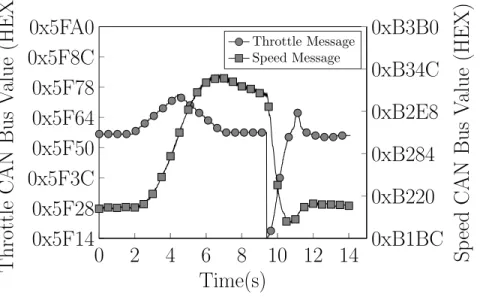
The connector diagrams in the Wiring Guide were used to determine the CAN bus connections to the PCM. These wires were cut and routed to the CAN injection platform. The CAN messages output from the PCM were recorded and passed through to the CAN bus for an accelerator pedal press. The recorded data was then played back on the bus and the vehicle accelerated as expected. Additional code was added to the playback function to selectively playback messages based on the message arbitration ID. This was used to search the recorded data set and isolate the acceleration control message. The messages were separated into two groups based on their arbitration ID, and each group was played back to the vehicle separately. The group that resulted in vehicle acceleration was separated again into two smaller groups and the process was repeated until one message arbitration ID was left. The acceleration control message was determined to be the message with arbitration ID 0x11A. Figs. 2.2and 2.3show successful CAN injections of the acceleration
control message, and the resulting speed for a ramp and step input, respectively. Due to the similarities between the acceleration control message, and a throttle signal in a gas powered car, this message is called the throttle message for the rest of this work.
Another approach to identify useful CAN messages for vehicle acceleration is by corre-lating the CAN messages with the vehicle speed. This approach was attempted by recording an accelerator pedal press and processing the data in Matlab. The CAN modules for the 2013 Ford Focus EV broadcast messages at prescribed frequencies as opposed to broad-casting in response to another signal. The speed message for the vehicle is broadcast at 100 Hz, which is the highest frequency messages are broadcast for this vehicle. Correlation was performed on messages of the same frequency, and the speed data was downsampled to perform correlation with messages at lower frequencies. The correlation returned a value between -1 and 1 for each byte of every message to indicate how closely correlated that byte was to the speed message. If the byte did not change during the recording, the correlation
returned NAN. On the EV-HS CAN bus there are 102 different messages and each message contains 8 bytes. The bytes were sorted based on the absolute value of the correlation value to identify the highest positively or negatively correlated bytes. The bytes that had aNAN
value were rejected and the final number of bytes being ranked was 341. The highest corre-lated byte of 0x11Awas byte 4, which had a correlation value of 0.2359 and was ranked 57
out of 341. The low correlation value and rank indicates that the throttle message would not have been identified using this strategy. In contrast, using the approach described in the previous paragraph, the throttle message was identified and was used to control vehicle acceleration.
The investigation of the braking system concluded that a CAN bus message about pedal position would not actuate the hydraulic braking system. The pedal signal is sent directly to the Automatic Braking System (ABS) CAN module, which is the only CAN module on the vehicle that is connected to the hydraulic brake lines. From this it was concluded that braking could not be fully controlled through the CAN bus.
The 2013 Ford Focus EV has an option to include park assist [38]. Though our specific vehicle did not include this option, it was determined that the Electric Power Assisted Steering (EPAS) system had the same part number and motor as the EPAS system in a vehicle with the park assist feature. This meant that the power steering motor would be powerful enough to turn the wheel at low speeds, and by extension, any speed. The Power Steering Control Module (PSCM) receives inputs from the CAN bus and the steering torque sensor located at the base of the steering column. The torque sensor uses a torsion bar to determine the amount of torque being applied by the driver, which is used by the PSCM to determine how much assist the power steering motor should provide. Simply, for a given torque input, less assistance would be provided by the EPAS system at higher speeds. Similar to the brake system, the input of interest is sent from a sensor to the module that performs the desired action. This led to the conclusion that the control of steering would have to be controlled through torque sensor input, and not through the CAN bus. In addition, the work by Miller and Valasek [29] [28] identifies the short comings of exploiting
0x5F14
0x5F28
0x5F3C
0x5F50
0x5F64
0x5F78
0x5F8C
0x5FA0
Throttle
CAN
Bus
V
alue
(HEX)
0
2
4
6
8 10 12 14
0xB1BC
0xB220
0xB284
0xB2E8
0xB34C
0xB3B0
Time(s)
Sp
eed
CAN
Bus
V
alue
(HEX)
Throttle Message Speed MessageFig. 2.2: CAN ramp injection from controller insertion point 1 and resulting vehicle speed. Data gathered from CAN bus and represented in hexadecimal format.
0x5EEC
0x5F14
0x5F3C
0x5F64
0x5F8C
0x5FB4
Throttle
CAN
Bus
V
alue
(HEX)
0
2
4
6
8 10 12 14
0xB1BC
0xB220
0xB284
0xB2E8
0xB34C
0xB3B0
0xB414
0xB478
Time(s)
Sp
eed
CAN
Bus
V
alue
(Hex)
Throttle Message Speed MessageFig. 2.3: CAN step injection from controller insertion point 1 and resulting vehicle speed. Data gathered from CAN bus and represented in hexadecimal format.
the park assist feature, namely, the park assist feature will cease to control the vehicle if the speed threshold is exceeded.
2.1.2 Sensor Emulation
The CAN bus injection method was unable to control braking and steering, so the sensor emulation method was explored. The accelerator pedal position sensor was analyzed to control vehicle acceleration, the brake pedal position sensor was analyzed to control the braking system, and the steering torque sensor was analyzed to control the vehicle steering. Fig. 2.4 shows these sensors and the following paragraphs discuss the analysis.
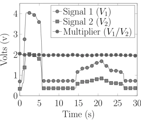
The accelerator pedal position (APP) sensor is located at the top of the accelerator pedal. There are six wires connected to the APP sensor, including two 5 V power wires with corresponding ground wires, and two signal wires. The sensor power pins were connected to a voltage source, and the signal wires were connected to an oscilloscope. It was determined that the sensor outputs two DC voltages similar to the output of potentiometers. Fig. 2.6
shows the voltage levels of the two output signals in response to a pedal press. The third signal on the graph is a multiplier that relates the two signals. It is seen that V1 ≈2V2.
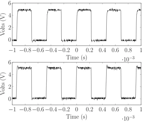
The brake pedal position (BPP) sensor is located at the top of the brake pedal. There are four wires connected to the BPP, including a 5 V power, ground, and two signal wires. The BPP was connected to the voltage source and oscilloscope in the same manner as the APP. However, the BPP outputs two PWM signals instead of DC voltage levels. When the brake pedal is not pressed the duty cycles of the signals settle at 89% for signal 1 and 11% for signal 2. During a braking event, the duty cycle for signal 1 decreases and the duty cycle for signal 2 increases at the same rate. Fig. 2.7 shows the two PWM signals for the BPP. The frequency of signal 1 is 533 Hz and the frequency of signal 2 is 482 Hz.
The steering torque sensor is located at the base of the steering column. The sensor connects to the Power Steering Control Module (PSCM) on the CAN bus, which determines the amount of power steering assist to provide. The assist is provided by an electric motor connected to the steering rack. In the sensor, a torsion bar is used to connect two parts of the steering shaft, where the rotational displacement can be measured to determine the
Fig. 2.4: The physical sensors emulated for vehicle control. Top: Steering rack for 2013 Ford Focus EV, the steering torque sensor is located at the base of the steering column and measures torque from driver. Bottom Left: The APP sensor located at the top of the accelerator pedal. Bottom Right: The BPP sensor that is usually mounted behind the brake pedal assembly and measures the brake pedal press.
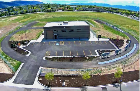
Fig. 2.5: Aerial view of the Electric Vehicle Roadway and Research Facility (EVR) at Utah State University.
0
5
10
15
20
25
30
0
1
2
3
4
Time (s)
V
olts
(v)
Signal 1 (V
1
)
Signal 2 (V
2
)
Multiplier (V
1
/V
2
)
Fig. 2.6: Acceleration pedal position sensor output. Two analog voltage signals related by
V1= 2V2.
−
5
−
4
−
3
−
2
−
1
0
1
2
3
4
5
·
10
−30
2
4
6
Time (s)
V
olts
(V)
−
5
−
4
−
3
−
2
−
1
0
1
2
3
4
5
·
10
−30
2
4
6
Time (s)
V
olts
(V)
Fig. 2.7: Brake pedal position sensor output signals. Signal 1: 89% resting duty cycle at 533 Hz. Signal 2: 11% resting duty cycle at 482 Hz.
torque input by the driver [39]. Similar to the BPP, there are 4 wires connected to the steering torque sensor, including 5 V power, ground, and two signal wires. The steering torque sensor was connected to the voltage source and oscilloscope, and it was determined that the sensor outputs two PWM signals on the signal wires, where both signals settle at 50% duty cycle when no torque is applied on the steering wheel. Both signals have a frequency of 2.15 kHz. Similar to the brake PWM signals, the duty cycles always add to 100%, and the direction that the steering wheel is being turned determines which signal’s duty cycle increases and which signal’s duty cycle decreases. Fig.2.8shows the two steering PWM signals.
2.1.3 Safety and Security
In 1996, the OBD-II (On-Board Diagnostics) specification was required to be imple-mented on any new vehicle sold in the United States [40]. This specification gives owners and technicians the ability to diagnose issues on the vehicle. The specification standardized connectors, message formats, and frequencies. The OBD-II port on the 2013 Ford Focus EV connects to the EV-HS CAN bus, which is the same bus that the throttle message is sent from the PCM to the TCM.
An attack platform was developed to inject arbitrary throttle messages through the diagnostics port. This attack method was important because, if successful, it would demon-strate that the acceleration of the vehicle could be controlled with limited intrusion. This differed from the approach in Section2.1.1, as it does not require access to the target mod-ule, or that the CAN wires be cut and re-routed. Instead, this platform could be plugged into the OBD-II port and monitor the bus for the target message arbitration ID. Also, it would show that if an attacker was able to inject messages from any module on the EV-HS CAN bus, then arbitrary vehicle acceleration could be caused. This would stand in contrast to the findings in [28], [29], [27], [26], where the acceleration of the vehicle could only be controlled under specific preconditions, and required intrusive access to the CAN bus.
The platform was connected to the CAN bus through the OBD-II port (other points on the bus could be used, as well) and monitored the traffic on the bus. The user determined a
−
1
−
0
.
8
−
0
.
6
−
0
.
4
−
0
.
2 0
0
.
2 0
.
4 0
.
6 0
.
8
1
·
10
−30
2
4
6
Time (s)
V
olts
(V)
−
1
−
0
.
8
−
0
.
6
−
0
.
4
−
0
.
2 0
0
.
2 0
.
4 0
.
6 0
.
8
1
·
10
−30
2
4
6
Time (s)
V
olts
(V)
Fig. 2.8: Steering torque sensor output signals. 50% resting duty cycles at 2.15 kHz.
target message, in this case, the throttle message, and provided that message arbitration ID to the system. In Section2.1.1, it was determined that the throttle message is included in the data frame associated with arbitration ID 0x11A, and is broadcast at 10 Hz. The platform waited until a message was received with the corresponding arbitration ID, and would replace throttle message data with an arbitrary throttle command value. The platform was designed to only alter the parts of the message that relate to the throttle control. The inserted message would be sent 250 µs after the actual message, leaving 9.75 ms for the inserted message to be received and processed by the TCM. This allowed the inserted message to dominate the period and cause the vehicle to accelerate. Fig. 2.9 shows the successful ramp injection through the OBD-II port and the resulting vehicle speed. Thus confirming the hypothesis that vehicle acceleration can be caused by injecting CAN messages through the OBD-II port, and therefore, could be caused at any other point on the bus.
These results demonstrate a CAN bus security concern. If an attacker were able to access the CAN bus, physically, or by compromising another ECU, they would be able
0
2
4
6
8 10 12 14
0x5F00
0x5F28
0x5F50
0x5F78
0x5FA0
Time (s)
Throttle
CAN
Bus
V
alue
(HEX)
0xB1BC
0xB220
0xB284
0xB2E8
0xB34C
0xB3B0
Sp
eed
CAN
Bus
V
alue
(Hex)
Car Throttle Message Injected Throttle Message Speed Message
Fig. 2.9: CAN ramp injection through OBD-II port with resulting vehicle speed. Injected throttle message was sent on bus immediately following car throttle message. Values read from CAN bus and displayed in hexadecimal format.
to effect the acceleration of the vehicle without causing any errors. Remote access to the vehicle, but not necessarily the requisite CAN bus, could be effected by compromising the Telematic Control Unit (TCU) or a wireless Tire Pressure Monitoring Sensor (TPMS). The TPMS sends a signal to the Body Control Module (BCM), which in turn transmits a message on the medium speed CAN bus (MS-CAN), while the TCU is connected to the I-CAN bus (it is unlikely, however, that compromising a sensor would allow for injection of arbitrary CAN messages onto the I-CAN or MS-CAN bus). These busses are connected to the EV-HS bus through a gateway module; transmitting a message from one bus to another, which would be required for either the TCU or TPMS to impersonate the PCM by passing APP messages, was not explored in this work. Regardless of the access approach, the driver is able to stop the unwanted acceleration by pressing the brake pedal. However, other works indicate that it is possible to make the vehicle ignore braking requests [29] [28] [26] [27]. This was not investigated as part of this work. Another security concern is that of a malicious technician. Since technicians will often access the OBD-II port when a vehicle is being serviced, it would be quite simple for them to leave an OBD-II injection platform connected to the OBD-II port. The acceleration control could be initiated remotely or by a timer,
causing the vehicle to accelerate at a dangerous time.
We present two remediation strategies that could be employed to help protect against this vulnerability. First, a simple change in the acceleration system architecture, such that the APP sensor connects directly to the TCM, which is the actuating module. This would remove the need of a throttle message to be sent from the PCM to the TCM and effectively remove the attack surface. The second approach is through device fingerprinting for both the digital and analog signals [41] [42]. This would allow the receiving module to authenticate the transmitting module, and prevent this type of attack.
CHAPTER 3
MODEL IDENTIFICATION AND LOW-LEVEL CONTROLLER DESIGN
This chapter provides an examination of the methods used for model identification of
the steering, braking, and acceleration systems in the 2013 Ford Focus Electric. Details are
given of the low-level controller design of desired velocity and steering wheel angle.
The efforts discussed in this chapter were led by the author of this work and his research partner, Austin Costley [30]. It is important to note the collaboration effort with Austin, and identify his contributions. In particular, Austin was instrumental in model identification and low-level controller design. This chapter was prepared for a coauthored journal submission with Austin. It is included in this thesis for completeness.
3.1 Model Identification and Low Level Controller Design
A simple overview of the control structure for the automated vehicle platform is shown in Fig.3.1. The high level controller plans the path and provides the desired vehicle speed,
vdesired, and desired steering wheel angle, θdesired. The low level controllers discussed in
this section are the inner loops that control vehicle speed and steering wheel angle. The vehicle commands are τcmd, AP Pcmd, andBP Pcmd, and represent, steering torque, APP,
and brake pedal position, respectively.
The first step in the development of the low level controllers was to determine a model of the system being controlled. A system model is expressed as a transfer function relating the input to the output of the system. Models were identified to relate the accelerator and brake pedal inputs to vehicle velocity, and steering wheel angle to vehicle heading. The following subsections review the model identification approach and low level controller design process for the Ford Focus.
3.1.1 Longitudinal Model
The longitudinal characteristics of the vehicle are affected by the APP sensor and the BPP sensor. These two systems were tested and identified separately, then implemented together as a complete longitudinal model.
In [43], Dias et al. perform longitudinal model identification and controller design for an autonomous vehicle. This approach was examined for the current work, however, a more straightforward classical controls technique using step responses was ultimately used. Once the acceleration and braking systems were identified, a control system was developed for each input device. The control loops for accelerator and braking were connected by switching logic to determine whether the accelerator or brakes should be used. A similar two loop control system with a switching logic component was used for the longitudinal controller in the current work. However, this work is an open-source project that uses the Robot Operating System (ROS) [44].
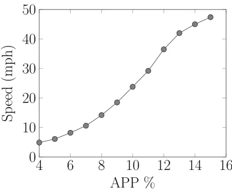
For the APP sensor system identification, the vehicle was placed on a dynamometer [45] and step inputs were initiated on the APP sensor from 4% to 15% at increments of 1%. Fig. 3.2 shows the step responses for some accelerator pedal inputs. It was observed that for a given APP percentage, the vehicle would eventually settle at a specific speed. The relationship between APP and speed can be described by a first order transfer function.
The general equation for a first order transfer function,G(s), can be represented by
G(s) = K
τ s+ 1, (3.1)
whereK is the constant or equation that relates APP to vehicle speed, andτ is the system time constant. The equation forK was derived from a linear fit of the a scatter plot of max speeds from the step input, as shown in Fig.3.3, and given by
f(x) = 3.65x−9.7, (3.2)
Differential Flatness Path Following
Algorithm
PID CompensationDeadband
Saturation Switching Logic PID Saturation Car τcmd + θd θer τ θm − vm − + vd ver +ver −ver AP Pcmd BP Pcmd Pose Longitudinal Controller Lateral Controller Path
Fig. 3.1: High-level system block diagram. Shows low-level control loop for lateral and longitudinal control and high-level differential flatness path following feedback loop.
0 20 40 60 80 100 120 140
0
10
20
30
40
50
Time (s)
Sp
eed
(mph)
5%
10%
15%
Fig. 3.2: APP step response for 5%, 10%, and 15% pedal presses. The graph shows a general first order speed response for a given pedal percentage.
4
6
8
10
12
14
16
0
10
20
30
40
50
APP %
Sp
eed
(mph)
Fig. 3.3: Vehicle settling speeds for given APP step input percentages.
4
6
8
10
12
14
16
0
5
10
15
APP %
Time
(s)
67
68
69
70
71
−
0.3
−
0.2
−
0.1
0
Time (s)
Deceleration
Rate
(m/s
2
)
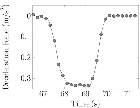
Fig. 3.5: Deceleration rate for BPP step input of 15%. The figure shows a first order relationship between BPP percentage and deceleration rate.
Fig.2.5) where the vehicle was operating is an oval track with sharp corners on the north and south side. The sharp corners and the short straightaways limit the vehicle operating speeds to between 15 and 25 mph for the initial automation. Theτ value that best represented the vehicle response between 15 and 25 mph was chosen as the time constant for accelerator pedal input in the longitudinal model. Fig. 3.4 shows the time constants for varying APP percentages. The time constant for the accelerator pedal input was chosen to be 7 seconds, as this best represented the system response for the nominal operating conditions. For BPP system identification, the vehicle was driven in a large, flat, asphalt area at speeds ranging from 5 to 25 mph at 5 mph increments. The vehicle was accelerated to the desired speed by a driver. Once the vehicle obtained the desired speed, an input to the braking system was initiated through the ROS setup discussed in Section5.1. Step inputs were initiated ranging from 5% to 50% of BPP percentage at increments of 5% for each speed value. The speed data seemed to show a consistent rate of change for a given BPP percentage. To confirm this, the speed data was smoothed using a 5 point moving average, and the derivative of the
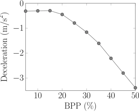
smoothed data was taken by calculating the difference between successive data points, and dividing by the elapsed time between data points. Fig. 3.5 shows the vehicle deceleration due to a braking event. It was observed that the settling value for the deceleration rate was consistent for a given BPP percentage and varying speeds, which concluded that the longitudinal model was independent of current vehicle speed. This speed independence can be seen in Fig.3.6where each line shows the deceleration rate for a given BPP percentage. At low BPP values, the lines converge, meaning that deceleration is unaffected by very small brake pedal percentages. However, at higher brake pedal percentages, the lines show distinct deceleration rates regardless of the vehicle speed. To show the relationship between BPP percentage and deceleration, an average was taken for each BPP value across each of the speeds. The result of this operation is shown in Fig. 3.7.
Similar to the APP model, the relationship between BPP and deceleration could be described by a first order transfer function. After analyzing the deceleration curves at dif-ferent BPP percentages and for difdif-ferent speeds, the system time constant,τ, was calculated to be 0.3 seconds. The equation that relates BPP to deceleration was determined by finding a curve fit algorithm for the curve in Fig.3.7. This would result in an equation that would provide a BPP percentage for a desired deceleration rate. The equation for K is given by
f(x) =−0.0018x2+ 0.029x−0.3768, (3.3)
where f(x) is the deceleration, and x is the BPP percentage. This equation is used to describeK from the general first order transfer function equation.
3.1.2 Lateral Model
The lateral model of the vehicle was determined by step response analysis. The model relates an input from the steering torque sensor to changes in the steering wheel angle. As discussed in Section2.1.2, the torque sensor measures the torque applied by the driver, and sends that information to the PSCM. The PSCM activates the power assist motor that connects to the steering rack, and moves the wheels. The steering wheel angle is measured
6 8 10 12 14 16 18 20 22 24
−
3
−
2
−
1
0
Speed (mph)
Deceleration
(m/s
2
)
15%
25%
30%
35%
40%
45%
50%
Fig. 3.6: Vehicle deceleration for BPP percentages at a variety of speeds. The values are the average of the deceleration rates settling point in response to a BPP step input. The lines for BPP percentages do not cross, and therefore, indicate speed independence for the brake model.
10
20
30
40
50
−
3
−
2
−
1
0
BPP (%)
Deceleration
(m/s
2
)
by a sensor in the steering wheel and output on the CAN bus at a high level of precision. Step inputs were initiated on the steering torque duty cycle signal ranging from 50% to 63% at 1% increments. Tests were performed at a large, flat, asphalt area with vehicle speeds ranging from 5 mph to 25 mph. Fig.3.8shows the results of the step input tests performed at 25 mph. It was observed that a general first order transfer function could be used to describe the relationship between steering torque duty cycle and steering wheel angle. However, at lower speeds and higher torque values, this observation is not valid. Fig. 3.9
shows the step response of the steering system at 15 mph. At the higher torque values, the steering wheel angles do not settle to a consistent steering wheel angle. It was also observed that the settling angles for a given steering torque duty cycle are not consistent for varying speeds. Therefore, the lateral model identification is speed dependent and would require a speed dependent limit on the steering torque duty cycle. Providing these characteristics, the system can still be modeled as first order transfer function for a given speed.
The steering data was analyzed in order to determine the gain equation, K, and the time constant,τ. Time constants were calculated for each step input response and for each speed. Fig. 3.10 Bottom shows the time constants for given steering torque duty cycles. Each of the lines indicates the speed at which the test was performed. It can be seen that at low speeds and low duty cycles the time constants are not consistent. But at higher speeds the inconsistencies lessen. A time constant, τ, of 0.2 seconds was chosen to optimize for typical vehicle operation.
Since the lateral system was found to be speed dependent, the gain equationK must also be speed dependent. The step input tests were performed at 5 mph increments so a gain equationK would be found for each speed value. These gain equations relate steering torque duty cycle to steering wheel angle. Fig. 3.10 shows the settling angles for varying steering torque duty cycles when the vehicle was traveling at 25 mph. A curve fit approximation was completed for this data set, and a solution was determined by solving the given equation. For this data set, the given equation for K is
0
0
.
5
1
1
.
5
2
2
.
5
3
0x1F4
0x3E8
0x5DC
0x7D0
0x9C4
0xBB8
0xDAC
Time (s)
Steering
Angle
from
CAN
Bus
(HEX)
58%
60%
62%
64%
Fig. 3.8: Steering torque step response for 58%, 60%, 62%, and 64% duty cycles at a vehicle speed of 25 mph. The plot indicates a first order relationship between torque duty cycle input and steering wheel angle.
0
0
.
5
1
1
.
5
2
2
.
5
3
0x7D0
0xFA0
0x1770
0x1F40
0x2710
0x2EE0
Time (s)
Steering
Angle
from
CAN
Bus
(HEX
)
58%
60%
62%
64%
Fig. 3.9: Steering torque step inputs for 58%, 60%, 62%, and 64% duty cycles at a vehicle speed of 15 mph. The plot indicates a first order relationship between torque duty cycle input and steering wheel angles, however, at high duty cycle percentages the first order relationship is not valid.
58
59
60
61
62
63
64
0x3E8
0x7D0
0xBB8
0xFA0
Duty Cycle (%)
Steering
Angle
(HEX)
58
60
62
64
66
68
70
0
1
2
3
Duty Cycle (%)
Time
(s)
5 mph
10 mph
15 mph
20 mph
25 mph
Fig. 3.10: Top: Steering angle settling values for given steering torque duty cycle step inputs. Values represented in hexadecimal format as received from CAN bus. Bottom:
Steering angle time constants for given steering torque duty cycle step inputs at varying speeds. The time constants converge at higher speeds.
wheref(x) is the steering wheel angle andx is the steering torque duty cycle.
Figs. 3.8 and 3.9 show the step response of the vehicle due to steering torque input signals. The graphs do not include step input values below 58% because the step responses at such values had little effect on the steering wheel angle. This exposed a deadband in the response from the steering torque sensor input to the steering wheel angle. A deadband compensation algorithm was implemented to mitigate the effects of this non-linearity. As shown in Fig.3.1, the deadband compensation code was executed just before the signal was sent to the vehicle. If the torque input value was greater than 50%, then
τcmd=Bmax+ τ−50
τmax−50
(τmax−Bmax) (3.5)
was used to compensate for the deadband. If the torque input value was less than 50%, then
τcmd =Bmin+
50−τ
50−τmin
(τmin−Bmin) (3.6)
was used to compensate for the deadband. Where τcmd is the torque command sent to
the vehicle, τ is the value received from the PI controller, Bmax is the upper limit of the
deadband,Bmin is the lower limit of the deadband,τmax is the maximum allowed value for
the steering torque signal, andτmin is the minimum allowed steering torque signal. For the
deadband on the 2013 Ford Focus EV, the upper and lower limits were 55% and 45%, and the maximum and minimum values for the torque signal were 64% and 37%, respectively.
3.1.3 PI Controller Design
Low-level control loops were designed to control vehicle speed and steering wheel angle. The desired speed and desired steering wheel angle would be input to the low-level control loops from a user or high-level controller. The low-level longitudinal controller interfaced with the accelerator and brake pedals to effect vehicle speed. A separate loop was designed for each vehicle input, and switching logic was used to choose whether the acceleration or brake loop would be used. The low-level lateral controller would receive the desired steering
wheel angle and determine the appropriate input to the steering torque sensor to achieve the desired angle.
A Proportional Integral (PI) Feedback Controller was implemented for longitudinal and lateral control. Fig.3.11shows a basic PI Feedback Controller for a first order system. The transfer function block represents the vehicle and contains the system model. The
1
K block effectively cancels out the gain equation K, and helps relate the speed error to a
vehicle input. For example, in the longitudinal controller, theK equation receives the APP as an input, and outputs speed. Therefore, the input to the transfer function block must be an APP value. However, the control loop is calculating a speed error, so the output of the PI block is a speed value. The K1 block translates the speed value into an appropriate APP value.
Since the K and K1 can be combined to equal 1, they can be ignored in the loop equation. The open loop transfer function of this system is then given by
GOL(s) =
1
(τ s+ 1). (3.7)
Closing the feedback loop and adding the PI controller gives
GCL(s) = kp τ s+ ki kp s2+1 τ + kp τ s+ki τ . (3.8)
PI
K1 τ sK+1in
out
−
Controller
Vehicle Model
The system is stable if the real part of the closed-loop poles are negative. Solving for the closed loop poles and zero yields
s= −(kp+ 1)± q kp+ 1 2 −4kiτ 2τ , (3.9) and s=−ki kp , (3.10)
respectively. From these equations it can be determined that if kp, and ki are positive the
system will be stable.
The second order transfer function obtained through closing the loop can be written, in a general form, as ω2 n s2+ 2ζω ns+ωn2 , (3.11)
whereζ is the damping coefficient andωnis the natural frequency. The damping coefficient
determines whether the system will be under-damped, over-damped, or critically damped and the natural frequency helps to determine the time constant for the system. The time constant,τ, is given by the equationτ = 1
ζωn. Values were chosen for the damping coefficient
and the time constant to define the system behavior. From these values one can determine the appropriatekp andki for the system. The equations for kp and ki are given by
kp =τ 2ζωn−1 τ , (3.12) and ki=τ ω2n, (3.13)
respectively. Table3.1shows the calculated values for each of the control inputs, where the
τcar column shows the time constants found during model identification and are internal
Table 3.1: Table of Values for Input Loops
Input τcar ζ τ ωn kp ki
Accelerator Pedal 7 1 0.5 2 27 28 Brake Pedal 0.3 1 0.5 2 0.2 1.2 Steering Torque 0.2 1 0.33 3 0.2 1.8
CHAPTER 4
LANE DETECTION AND VISION-BASED CONTROL
This chapter details the methods for lane detection and the design of an accompanying
vision-based controller which uses lane information to navigate within the roadway.
4.1 Lane Detection
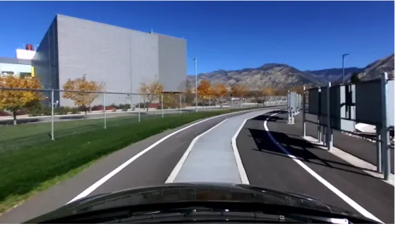
Lane detection is an essential part of navigating urban roadways. Although it is in-tuitive for humans to identify and follow lane markers, machines are plagued with many obstacles in the performing the task. Difficulties include varying road types and markers, changes in weather and lighting conditions, and other vehicles obscuring the view of the road. This work focuses on detecting the lanes on the closed circuit test track at Utah State University’s EVR [46]. While there are no other vehicles to obstruct the lane markers, the track presents challenges in lane detection as shown in Fig. 4.1. Charging gutters in the middle section of the road are surrounded by cement strips similar in width and color to lane markers. Curves on either end of the track are sharper than those found in highway driving and most standard roadways. Charging equipment near the side of the road casts shadows on the lane markers, making them more difficult to detect. Extensive work on detecting lane markers in urban roadways was performed by Aly [14]. A modified version of his algorithm is presented in this section.
4.1.1 Inverse Perspective Mapping
Images received by a camera suffer from what is known as the perspective effect. Lines which are parallel in the world frame do not run parallel in an image taken from a camera mounted on a vehicle. Instead, they converge at the horizon as can be seen in Fig. 4.1. Furthermore, without knowing an object’s size, there is not a measure of distance for a monocular image. Inverse Perspective Mapping is a technique which resolves the perspective
Fig. 4.1: Original image taken on EVR test track. Difficulties for lane detection are shown including shadows, a steep curvature, and shapes similar to lane markers in the center of the road
problem by creating a top-view perspective of a forward facing image. This bird’s-eye view has distinct advantages in lane detection. After an IPM transform, lanes which run parallel in the world frame are also represented as parallel in the image frame. IPM give a sense of depth and maps a pixel to meter distance for the image. It also focuses on a subregion of the original image, decreasing the computational processing needed.
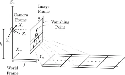
IPM is a geometric transformation which uses camera intrinsics and extrinsic to display a bird’s-eye view of the image. Intrinsic parameters include camera focal length and focal center. Camera height, pitch, and yaw are taken into account for extrinsic parameters. Fig.4.2shows IPM operates in three frames: a world frame{Fw}={Xw, Yw, Zw}centered
at the camera’s optical center, a camera frame {Fc} = {Xc, Yc, Zc}, and an image frame {Fi} = {u, v}. Pitch angle α and yaw angle β are allowed for, but no roll angle. It is assumed the camera’sXc axis stays in the world frame’sXwYw plane. The camera’s height
above the ground plane is defined as h. The road surface is assumed to be flat. From any point in the image planeiP ={u, v,1,1}, it’s projection on the road plane can be found by
Vanishing Point Zw Yw Xw f World Frame u v Image Frame h Zc Xc Yc Camera Frame
Fig. 4.2: Inverse Perspective Mapping (IPM) frames. IPM is a geometric transformation which maps a 2D image to a 3D world frame
applying the homogeneous transformation g iT =h −1 fuc2 1 fvs1s2 1 fucuc2− 1 fvcvs1s2−c1s2 0 1 fus2 1 fvs1c1 − 1 fucus2− 1 fvcvs1c2−c1s2 0 0 1 fvc1 1 fvcvc1+s1 0 0 −hf1 vc1 1 hfvcvc1− 1 hs1 0 (4.1)
where c1 = cosα, c2 = cosβ, s1 = sinα, and s2 = sinβ. The horizontal and vertical
focal lengths are {fu, fv} and the coordinates of the optical center are {cu, cv}. With this
transformation, gP = giTiP is the point on the ground plane corresponding to iP in the image plane. The same holds for the inverse of the transform
i gT = fuc2+cuc1s2 cuc1c2−s2fu −cus1 0 s2(cvc1+fvs1) c2(cvc1+fvs1) −fvc1−cvs1 0 c1s2 c1c2 −s1 0 c1s2 c1c2 −s1 0 (4.2)
where a point in the ground plane gP ={x
g, yg,−h,1} can be obtained in the image
frame by iP =i
gTgP, followed by a rescaling of the homogeneous part. Fig. 4.3 shows an
example of taking the IPM transform of Fig.4.1. The original image has a size of 1280x720 and the transformed image has a size of 360x240. As mentioned before, the lanes in Fig.4.3
now appear parallel and have a fixed width.
4.1.2 Filtering and Thresholding
After the IPM transform, the image is filtered horizontally using a second derivative Gaussian filter: fu(x) = σ12 xexp(− x2 2δ2 x)(1− x2 δ2
x). This is designed to accentuate bright areas
on a dark background, following our assumption of a lane marker’s appearance in the image. The filter is tuned to keep vertical lines of a lane maker’s width. The filter also keeps quasi-vertical lines. Fig. 4.4 shows the filter applied to Fig. 4.3. It can be seen that lane data is kept well along with other parts of the image with similar attributes. Although Aly [14]
Fig. 4.4: Image filtered using a second derivative Gaussian horizontal kernel
Fig. 4.5: Thresholded image retaining high intensity areas. The image is not binarized and keeps all intensity values above the threshold
suggests a vertical smoothing filter, one was not used in our implementation because it did not significantly increase the effectiveness of the filter.
Thresholding is performed on the filtered image, keeping only the highest values. The average pixel value is calculated for the filtered image, and values below it’s q% are set to zero. A Value ofq = 97.5 was used for the images in this chapter. It is important to note that the thresholded image is not binarized. Pixel values above the threshold are kept to preserve intensity data. Fig.4.5is the result of this thresholding method on Fig.4.4. Lane markers are easily seen in the image with the exception of shadow areas.
4.1.3 Line Fitting
For the thresholded image, pixels are summed vertically for each column. The result is smoothed by a Gaussian filter and the local maxima are detected as shown in Fig.4.6. The lines are grouped to account for multiple entries and the resulting lines (Fig. 4.7) are used as the basis for line and spline detection. A bounding box is taken around each of these lines and a line is fit using RANSAC for the data within the bounding box. Fig.4.8shows a line fit to a sub-image defined by a bounding box around one of the lines in Fig.4.7. The same process is run for each of the bounding regions and produce a line fit by RANSAC for each. Fig. 4.9shows the combination of all lines fit.
4.1.4 Spline Fitting
Algorithm 1 RANSAC Spline Fitting
1: fori=1 to numIterations do
2: points=getRandomSample() 3: spline=fitSpline(points)
4: score=computeSplineScore(spline) 5: if score > bestScorethen
6: bestSpline=spline
7: end if
8: end for
Fig. 4.6: Local maxima of image columns. Pixel values are summed vertically. Local maxima are indicated by the red lines
Fig. 4.7: Vertical lines indicating the subregions of interest in image. A bounding box is taken around each line and a curve is fit for all data within the bounding region
Fig. 4.8: Region showing line fit by RANSAC to potential lane data
Fig. 4.9: Lines fit to subregions of image. These lines are used as initial guesses for RANSAC spline fitting
Fig. 4.10: RANSAC fitting of spline to subregion data. The current iteration is shown in red while the best fit spline is shown in blue
P1 P2 P3 P4
l
θ1 θ2Fig. 4.11: Third degree Bezier Spline consisting of four control points. A measure of straightness is estimated through θ1 and θ2 and length is defined as l
is fit to that data, with the line used to determine a new bounding region. A RANSAC spline fitting method is used to robustly fit a spline. A third degree Bezier spline is used to fit this data and is defined by
Q(t) =T(t)M P (4.3) Q(t) = t3 t2 t 1 −1 3 −3 1 3 −6 3 0 −3 3 0 0 1 0 0 0 P0 P1 P2 P3 (4.4)
wheret∈[0,1],Q(0) =P0,Q(1) =P3, andP1andP2are control points that determine
the shape of the spline as can be seen in Fig. 4.11. The RANSAC method is outlined in Algorithm 1and makes use of the following functions:
1. getRandomSample(): This function randomly selects n points from the sub-image Points are weighted according to the filtered and thresholded value such that points with a higher weight have a greater likelihood of being selected by getRandsomSam-ple().
2. fitSpline(): Points supplied by the previous function are fit to a third degree Bezier spline using a least squares method. For each ofnpoints, a valueti∈[0,1] is assigned
to each point pi = (ui, vi) in the sample, where ti is proportional to the cumulative
sum of the euclidean distances from point