Evolutionary deep belief networks with bootstrap sampling
for imbalanced class datasets
A’inur A’fifah Amri a,1, Amelia Ritahani Ismail a,2,*, Omar Abdelaziz Mohammad a,3 a Department of Computer Science, Kulliyyah of Information & Communication Technology,
International Islamic University Malaysia, Kuala Lumpur, Malaysia
1[email protected]; 2 [email protected]; 3 [email protected]
* corresponding author
1.
Introduction
An imbalanced class can affect negatively in the decision-making process by providing poor results due to misclassification and fluctuating error rates [1]. Common methods used to overcome such problem are by data sampling or algorithm modeling [2]. The data sampling method is commonly used and is useful when it comes to handling the imbalanced class issue because it deals with the problem directly. The basic approach that is frequently used is undersampling or oversampling. However, the issue with undersampling is that it is possible to get rid of crucial data needed for prediction [3], while the issue with oversampling is that it causes overfitting in learning [4]. Nevertheless, implementing a data sampling method is still sought after since it can minimize the negative effects of imbalanced class problems because it deals with the data directly. Another plausible solution for an imbalanced class problem is by algorithm modeling. Deep learning has shown promising results in many domains, especially the ones that require high-level abstraction and has complex data features, such as image processing, emotion detection and handwriting recognition [5]–[7]. An example of deep learning algorithms is a deep belief network (DBN). DBN can learn from complex feature input such as emotion recognition [7] and acoustic modeling [8]. Therefore, it can learn the features from an imbalanced class dataset and classify it correctly. Despite the promising performance of DBN in various fields, the algorithm is generally computationally expensive and unable to achieve a competent result when learning from an inadequate amount of data [7], [8].
Imbalanced class ordeal in a dataset is a common classification task problem. According to references
[4] and [9]–[12], imbalanced class refers to the “disparity of data dispensation between the classes”. The class that has more training values is called the majority class and the class that has the least or most missing data values are called the minority class [13]. Minority data class is a realistic problem that the A R T I C L E I N F O A B S T R A C T
Article history Received July 23, 2018 Revised December 3, 2018 Accepted December 20, 2018 Available online July 26, 2019
Imbalanced class data is a common issue faced in classification tasks. Deep Belief Networks (DBN) is a promising deep learning algorithm when learning from complex feature input. However, when handling imbalanced class data, DBN encounters low performance as other machine learning algorithms. In this paper, the genetic algorithm (GA) and bootstrap sampling are incorporated into DBN to lessen the drawbacks occurs when imbalanced class datasets are used. The performance of the proposed algorithm is compared with DBN and is evaluated using performance metrics. The results showed that there is an improvement in performance when Evolutionary DBN with bootstrap sampling is used to handle imbalanced class datasets.
This is an open access article under the CC–BY-SA license.
Keywords Imbalanced class Deep belief networks Genetic algorithm Bootstrapping sampling Complex feature input
real-world situation faced because most of the time even for an important dataset such as cancer detection
[14] and bank fraud [15], the data instances are scarce. It can be expensive if the new data needs labeling
[16]. Unfortunately, most of the algorithms that showed stable and promising performance when using balanced data in classification tasks displayed conflicting outcome when the imbalanced class dataset is used [17]. Prediction of minority class is presumed to have a higher error rate compared to the majority class and its test examples are often wrongly classified as well [1]. Imbalanced data distribution among the classes causes deficient classification models [11]. The algorithm that performs on a balanced dataset will not perform as good when using an imbalanced dataset [9], regardless of how good the model is. In a study done by Yan et al. [10], an imbalanced class dataset in multimedia format is implemented as the input for CNN. The dataset is a TRECVID dataset, which means it is in the form of video. The outcome shows that the error rate fluctuate unlike when using a balanced dataset, the error rate of the algorithm decrease steadily. There are a few commonly used methods utilized to tackle the challenges of the imbalanced class dataset. The first method is using machine learning algorithm and model hybrids according to the input types [2], [12]. Another method is by data preprocessing of the imbalanced dataset itself [2].
Bootstrap sampling is when a small sample is derived from its original sample iteratively [10], [18]. This method basically reuses its training samples and this is a suitable technique to avoid data redundancy as well as data disposal. Megumi et al. [19] conducted a neuroscience experiment involving fMRI neurofeedback. Bootstrap sampling was utilized as a method to assess the experiment’s difference in correlation between the neurofeedback and other networks. Bootstrapping sampling is a frequently adopted technique implemented to improve the performance of deep learning algorithms with imbalanced class data [4], [16]. Yan et al. [10] implemented the convolutional neural network (CNN) to classify an imbalanced multimedia dataset. The bootstrap sampling method is integrated with the algorithm to minimize its fluctuating error rate. The experiment yielded high F1-score as compared to another framework proposed by Tokyo Institute of Technology (TiTech). In another literature, Berry et al. [16] implemented bootstrap sampling as a method to improve both computational time and accuracy rate after training the imbalanced and unlabeled data using deep belief network (DBN). The result is recorded to have a 41% decrease in an error rate that needs human intervention as compared to no bootstrapping implementation. Sun et al. [20] predict wind speed and wind power using deep belief network and optimized random forest. The experiment has an inconsistent amount of data because some data are simply unavailable. Therefore, the experiment employed bootstrap sampling as an approach to resampling the training data to improve the performance of their model.
A deep belief network (DBN) is made up of a stack Restricted Boltzmann Machine (RBM) for network pre-training and implement a backpropagation neural network (BPNN) as a fine-tuning step. The RBM architecture connects the hidden layers and visible layers bidirectionally. This two-way connection between the layers results in deeper extraction between the neurons as the weights are connected exclusively. RBM is probabilistic [21], which means that RBM units are assigned statistically random with values 0 or 1. Its two-layer, bipartite, undirected graphical model has a set of binary hidden random variables h of dimension K, a set of binary or real-valued visible random variables v of dimension D. The symmetric connections of the two layers are represented by a weight matrix [22]. According to Zheng et al. [23], the output layer of the lower-level layer in the RBM will be the input layer to its higher-level layer in a bottom-up manner to allow the pre-training of weight occurs within the DBN. This feature contributes to an increase in accuracy level. There are two common types of RBM [7], which are Bernoulli RBM and Gaussian RBM. Bernoulli RBM has binary values for its hidden and visible layers, whereas Gaussian RBM has real number values for its hidden and visible layers.
DBN is a composition of simple learning modules, RBM, in a bottom-up way. The RBMs in DBN is trained per layer in a greedy manner [24]. DBN’s generative pre-training adds a higher level of feature abstraction of the input in the network. Neural network layers are exponentially dense [8], but the deepness of DBN allows low-level feature abstraction handled by the lower layers and the high level or nonlinear feature abstraction handled by the higher layers of the network. However, this made DBN computationally expensive and time-consuming due to its number of layers. According to an experiment done by Le and Provost [7], training a DBN is expensive in terms of computation because pre-training
took 11 minutes per epoch, and fine-tuning takes up 10 minutes per epoch. Time is taken to feature extract using DBN for speech emotion recognition cost 136 hours. Plus, it is longer when compared to other methods for the dataset [25]. Generative pre-training of weights in DBN is essential to augment the possibilities of the input through layers from below [8]to make it more accurate, but this results in an expensive computation of the network. According to Hinton [26], this setback can be minimized by applying “contrastive divergence” on every layer. Another common problem with DBN is the parameter setting [27]. There is much effort to combine the settings of DBN, finally, to get the best performance. Although DBN shows it can learn from imbalanced class dataset better than CNN, the time taken for training is long [28]. A financial distress prediction using real-life dataset implements a DBN hybrid to perform the prediction [29]. The dataset is classified into two categories, distressed and non-distressed for “Micro-business” and “Small and Medium Business” (SMB), and the ratio is stated to be imbalanced. RBM feature on a DBN is used in a pre-training data, and SVM is employed for classification phase. The result is 76.8% accurate as compared to 62.1% by ANN. Berry et al. [16] utilized DBN to cater to imbalanced unlabeled data. The dataset consists of ultrasound images of tongue when a subject is performing human speech. Imbalanced in speech data is simply unavoidable because some images will look similar than the rest as stated in Zipf’s Law. Bootstrapping is incorporated into DBN to reduce computation time. The method proves to improve the accuracy and reduced time taken for labeling the data. Kuang and He [30] attempted to classify fMRI datasets using DBN to predict whether a patient has ADHD or not. The ADHD dataset is imbalanced, and its effect on DBN is low accuracy rate. Therefore, the dataset went through preprocessing methods and this approach saw an increase of accuracy rate using DBN.
Genetic algorithm (GA) is a heuristic search algorithm that models from the biological evolution
[31], [32] introduced by John Holland in the 1970s. GA mimics the human genetic mutation and selection process [33]. GA is made up of the chromosome. A chromosome contains multiple genes, and a collection of chromosomes is called a population [31]–[34]. The objective of GA is to ensure that the next iteration has better chromosomes that its previous ones. Therefore, a selection of fitness functions is used as a yardstick to verify that the process is successful. It has various mapping techniques and fitness measurements [35]. The crossover and mutation features of GA creates randomness in the population allows the heuristics to avoid local optima solutions [36]. Liu et al. [34] state that it is an ideal algorithm to be used in fields such as optimization and forecast.
In the latest researches, GA is commonly used to improve or a part of a hybrid algorithm when it comes to prediction and classification. GA has been used as a hybrid with a Particle Swarm Optimization (PSO) to improve a feature selection process of the Indian Pines hyperspectral data set [33]. Jamshidi et al. [35] have used GA as a part of optimization in removing an element in the chemistry domain. GA is also used to optimize SVM in an application using a wavelet transform to forecast short-term wind speed
[34]. Other than that, GA is utilized as an optimization for CMP [32]. Elhoseny et al. [37] have employed GA to balance the energy consumption in WSN domain. The data used is heterogeneous. GA is applied in as a feature selection for a credit risk assessment based on a bank in Croatia [38]. Neath et al. [39]
applied GA to obtain the ideal level of performance for the proportional-integral-derivative (PID) controller by tuning its parameter. Assodiky et al. [40] used GA as a feature selection as a part of an H20 Deep Learning in order to classify ECG data to detect Arrhythmia. Inanlo and Zadeh [41] applied classification on social networks using GA-based DBN. The network has converged properly and is stable to classify social networks dataset. For the imbalanced data classification task, GA is used efficiently to overcome the common problems through its selective feature. Deshmukh and Akarte [42] has used GA as an approach to improve SVM for its imbalanced medical data task. Haque et al. [36] took an approach to use a heterogeneous Ensemble of Classifiers (EoC) in order to overcome the imbalanced data problem through generalization. The authors proposed a GA-based technique to appoint the best classifiers that will build a good heterogenous EoC and acquired better result than base classifier and other ensembles. Another method to deal with the imbalanced dataset is by using the cost matrix method. Perry et al.
[43] integrated GA to produce cost matrices that will allow the algorithm to deal with different use-cases of imbalanced data efficiently. GA is known to be robust and a good optimization algorithm [34]. Haque et al. [36] stated that GA is suitable for tasks that are massive and elaborate because it is less likely
to get stuck in local optima, unlike other heuristics. However, Asadi et al. [44] claim that GA is computationally expensive when an evaluation function needs to be executed many times. Therefore, the overall context of the datasets needs to be taken into account if the algorithm aims to be cost-sensitive.
In this paper, an optimized DBN is proposed to control the negative outcomes caused by imbalanced class data towards the performance of the algorithm using an evolutionary algorithm. An evolutionary algorithm (EA) is incorporated to provide the optimum dropout number, learning rate, batch size, and iteration number of BPNN for fine-tuning in DBN. Bootstrap sampling is also incorporated in the algorithm structure to minimize the bias of data training samples. These modifications improved the ability to predict more accurate outcomes for the imbalance dataset.
2.
Method
2.1.The Proposed Method
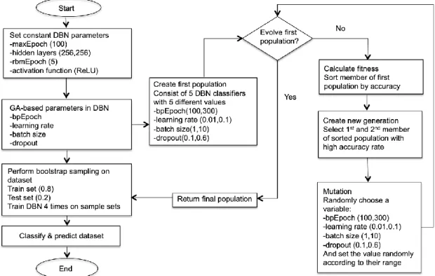
DBN shows the good result when dealing with inputs of the complex feature. However, the result of DBN in predicting imbalanced class datasets is unstable. This paper proposes GA and bootstrap sampling as a part of DBN to minimize the shortcomings. Fig. 1 explains the modification performed on DBN.
Fig. 1. Flowchart of Evolutionary DBN with bootstrap sampling
In Evolutionary DBN with bootstrap sampling, the algorithm receives an imbalanced class dataset as input. The instances of the data are taken and split up into training and testing set using cross-validation. The testing set of the dataset is assigned to 0.2, which means 80% of the dataset is used for training, and 20% is left out and is used for testing. The maximum epoch is set to 100. One epoch will take the inputs as neurons and calculate the weights and biases into the connected hidden layers. One node of a neuron consists of initialized weights and calculated with activation function, rectifier linear unit (ReLU). The output of one neuron is an input for another neuron, which allows the network to learn. The input will go through a network of connected RBM for the pre-training phase and backpropagation neural network (BPNN) for fine-tuning phase. Then, the weights will be adjusted for the next epoch as per trained by the previous epoch. After the calculated weights are adjusted, the network will iterate the same process of calculation and keep adjusting the weights until the maximum epoch is reached. The
weights are responsible for the network to make a decision and predict the output as trained using the training data. In the algorithm, pre-training using RBM is set to 5. The DBN classifier is assigned with 2 hidden layers that consist of 256 neurons per hidden layer. Genetic algorithm (GA) is employed as the evolutionary part of Evolutionary DBN with bootstrap sampling. The main steps of GA are initializing population, calculate the fitness of the individuals in the current population, creating a new population and the fitness of its individuals are calculated and compared with the previous population. Next, the individuals with the best fitness value will be mutated and evolved for the next generation. The procedure is repeated until termination. In this algorithm, GA initializes the population of 5 DBN classifiers with randomized parameters. The parameters improved using GA approach are the BPNN iteration number, the learning rate of the network, batch size, and dropout number. The population underwent an evolutionary process where the fitness calculation is performed. The classifier with the best and second-best fitness value is selected as a new generation. Then, this new generation went through a mutation process where GA chose a parameter of the best classifier randomly and assigned the value randomly according to its value range. In this case, the BPNN iteration number is set between 100 to 300, the learning rate is between 0.01 and 0.1, the batch size is set between 1 to 10 and dropout size is between 0.1 and 0.6. After this evolution process, the algorithm returns a GA optimized DBN and performed bootstrap sampling. Bootstrap sampling is implemented after an evolutionary DBN classifier has optimized its parameter setting. The classifier will train itself using the initial training data split. Then, the dataset gets reshuffled using the same ratio utilized for the initial training data. The classifier will retrain itself again. This process repeats until the fourth time. This is the optimal sampling number for Evolutionary DBN. As the maximum epoch reached, the testing set is used to test the algorithm performance. The algorithm predicts and classifies the output according to its learning performance.
Performance metrics such as accuracy rate, weighted mean precision, weighted mean recall, and F1-score is computed and taken as a measure to evaluate the overall implementation of Evolutionary DBN with bootstrap sampling. The accuracy rate is the total number of correctly classified over the total number of samples. The formula for the accuracy rate is shown in (1).
𝐴𝑐𝑐𝑢𝑟𝑎𝑐𝑦 = 𝑇𝑃
𝑇𝑃+𝑇𝑁+𝐹𝑃+𝐹𝑁
Where TP is true positives, TN is true negatives, FP is false positives, and FN is false negatives. However, the accuracy rate alone is not enough to review the performance when handling imbalanced class datasets. Therefore, weighted mean recall of the algorithm is taken into account to ensure there is no bias when it comes to recalling samples from minority class [45]. The formula for the weighted mean recall is as shown in (2).
𝑅𝑒𝑐𝑎𝑙𝑙 = 𝑇𝑃
𝑇𝑃+𝑇𝑁
Weighted mean precision indicates the preciseness of the algorithm for each imbalanced class datasets. The formula is shown in (3).
𝑃𝑟𝑒𝑐𝑖𝑠𝑖𝑜𝑛 = 𝑇𝑃
𝑇𝑃+𝐹𝑃
F1-score evaluate the harmonic value between recall and precision. This metric is useful to find the balance between the biased of an algorithm with its preciseness when classifying instances in the correct category. The formula of F1-score is shown in (4).
𝐹1 − 𝑠𝑐𝑜𝑟𝑒 = 2 ×𝑃𝑟𝑒𝑐𝑖𝑠𝑖𝑜𝑛 × 𝑅𝑒𝑐𝑎𝑙𝑙
𝑃𝑟𝑒𝑐𝑖𝑠𝑖𝑜𝑛+𝑅𝑒𝑐𝑎𝑙𝑙
2.2.Datasets
This section presents the imbalanced class datasets used for the experiment. The datasets are chosen based on the data disparity of the instances between their classes. The datasets are also chosen based on
similar studies using the same datasets conducted by Weiss and Provost [1], Zhang et al. [46], Boughorbel et al. [47], and Lopez et al. [48].
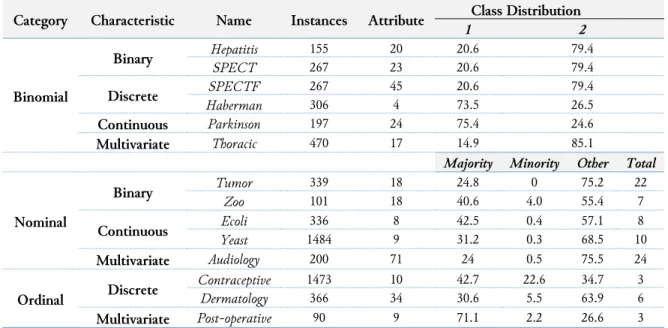
Table 1 shows the distribution of the imbalanced class datasets. The instances are the number of items in the dataset. The number of the attribute includes the class. Missing values are disposed from the datasets. The imbalance pairings for the datasets range between 15-85, 20-80 and 75-25 for binomial category datasets. The distribution ratios are not balanced either by 50-50 or 40-60 pairing. The datasets with a huge gap of the ratio are more exposed to encounter biased prediction as compared to a dataset with a smaller ratio gap. For multiclass datasets, the data are divided into nominal and ordinal categories. Nominal is when a dataset label has more than two classes. Ordinal data is also when the instances can be classified into more than two classes but in an ordered form. The instances are sorted into each class according to the attributes it satisfies. It presents the distribution of the majority class, minority class and other classes in the dataset. This is because all the imbalanced class datasets in the multiclass category have a varied number of classes. Therefore, it might not clear to see the difference between the majority and minority classes if the data distribution is presented according to each class
Table 1. Details and distribution of Imbalanced Class Datasets
Category Characteristic Name Instances Attribute Class Distribution
1 2 Binomial Binary Hepatitis 155 20 20.6 79.4 SPECT 267 23 20.6 79.4 Discrete SPECTF 267 45 20.6 79.4 Haberman 306 4 73.5 26.5 Continuous Parkinson 197 24 75.4 24.6 Multivariate Thoracic 470 17 14.9 85.1
Majority Minority Other Total
Nominal Binary Tumor 339 18 24.8 0 75.2 22 Zoo 101 18 40.6 4.0 55.4 7 Continuous Ecoli 336 8 42.5 0.4 57.1 8 Yeast 1484 9 31.2 0.3 68.5 10 Multivariate Audiology 200 71 24 0.5 75.5 24 Ordinal Discrete Contraceptive 1473 10 42.7 22.6 34.7 3 Dermatology 366 34 30.6 5.5 63.9 6 Multivariate Post-operative 90 9 71.1 2.2 26.6 3
3.
Results and Discussion
This section presents the results of Evolutionary DBN with bootstrap sampling to classify imbalanced class datasets and its comparison to other algorithms such as DBN and DNN. Performance metrics used to evaluate the performance of Evolutionary DBN with bootstrap sampling are accuracy rate, weighted mean recall, weighted mean precision, and F1-score. The results are recorded in the respective tables and are analyzed.
3.1.Accuracy Rate
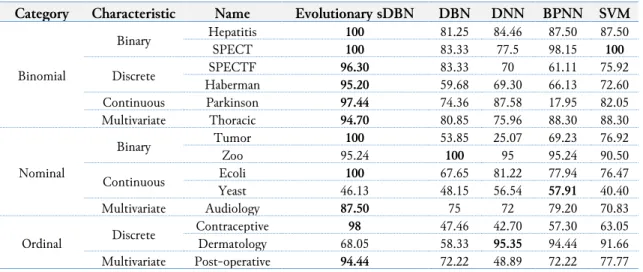
Table 2 depicts the accuracy rate achieved for each algorithm for each imbalanced class dataset used in this experiment. The result is discussed according to the category of the imbalanced class datasets. For binomial category, the proposed Evolutionary DBN with bootstrap sampling achieved the highest accuracy rate contrast to other algorithms used for comparison, with an exception for SPECT dataset where SVM also achieved a high accuracy score. SVM manage to score a high accuracy rate for the dataset mentioned because the attributes of the dataset are in binary form, which is suitable for SVM hyperplane approach. If we compare DBN result to other algorithms such as DNN, BPNN, and SVM, the algorithm only score the highest when dataset SPECTF is used in the experiment. Therefore, Evolutionary DBN with bootstrap sampling managed to improve the performance of DBN when predicting the output of imbalanced binomial dataset. DBN manage to achieve the highest accuracy
using SPECTF data because it has the most attributes. Therefore, it is only ideal for DBN to perform when the algorithm has many features to learn. Evolutionary DBN with bootstrap sampling overcome this specific requirement for DBN to perform and achieve the highest accuracy rate in all imbalanced class dataset in a binomial category.
Table 2. Accuracy Rate of Algorithms
Category Characteristic Name Evolutionary sDBN DBN DNN BPNN SVM
Binomial Binary Hepatitis 100 81.25 84.46 87.50 87.50 SPECT 100 83.33 77.5 98.15 100 Discrete SPECTF 96.30 83.33 70 61.11 75.92 Haberman 95.20 59.68 69.30 66.13 72.60 Continuous Parkinson 97.44 74.36 87.58 17.95 82.05 Multivariate Thoracic 94.70 80.85 75.96 88.30 88.30 Nominal Binary Tumor 100 53.85 25.07 69.23 76.92 Zoo 95.24 100 95 95.24 90.50 Continuous Ecoli 100 67.65 81.22 77.94 76.47 Yeast 46.13 48.15 56.54 57.91 40.40 Multivariate Audiology 87.50 75 72 79.20 70.83 Ordinal Discrete Contraceptive 98 47.46 42.70 57.30 63.05 Dermatology 68.05 58.33 95.35 94.44 91.66 Multivariate Post-operative 94.44 72.22 48.89 72.22 77.77
In the nominal category, Evolutionary DBN with bootstrap sampling attained the highest accuracy rate for imbalanced datasets, Tumor, Ecoli and Audiology, which accounts for 3 out of 5 nominal datasets. For binary attributes in the nominal category, Evolutionary DBN with bootstrap sampling accomplished high accuracy rate for Tumor dataset, but second-highest for Zoo dataset alongside with BPNN. DBN scored the highest accuracy rate for Zoo dataset. For continuous numerical attributes in the nominal category, Evolutionary DBN with bootstrap sampling accomplished high accuracy rate for Ecoli dataset, but second lowest for Yeast dataset. Ecoli has 8 attributes in contrast to Yeast with 9 attributes. The instances are 336 and 1484, respectively. Ecoli dataset has 8 classes as compared to 9 classes of Yeast dataset. The parallel comparison between the binary and continuous numerical attributes shows that the number of instances, attributes, and a total class of the imbalanced datasets are not the factors influencing the performance achieved by Evolutionary DBN with bootstrap sampling. However, for the classes in Zoo dataset, although there are 7 classes, each of the class comprised of different animals that share a similar attribute but not necessarily from the same species. For example, Class 2 consists of 20 bird-like species such as “chicken”, “penguin”, and “vulture” among others. The shared attributes for these animals might be “2 legs” and “eggs”, but a “penguin” is labeled “aquatic” as opposed to a “vulture” is labeled “airborne”, while “chicken” is not labeled with such attributes. They are all considered in Class 2. This sort of structure in the dataset might cause Evolutionary DBN with bootstrap sampling unable to achieve 100% accuracy rate as compared to DBN. For continuous numerical attribute, it is important to note that for Yeast dataset, where Evolutionary DBN with bootstrap sampling achieved second-lowest accuracy result yields very low accuracy rate from other algorithms as well with BPNN scored the highest at 57.91%.
In ordinal category, Evolutionary DBN with bootstrap sampling obtained the highest accuracy rate for 2 out of 3 imbalanced class datasets, which are Contraceptive and Post-operative datasets. For Dermatology dataset, the algorithm achieved the second-lowest accuracy result, and DBN is the lowest accurate as compared to DNN, BPNN, and SVM, which has between 91% and 95% accuracy range. Even though there is an increment of about 10% in accuracy, but it can be concluded that DBN structure unable to learn from the dataset attributes. As for Contraceptive dataset, Evolutionary DBN with bootstrap sampling achieved 98% accuracy as compared to DBN at 47.46% and other algorithms ranges between 42% and 63%, this shows a huge improvement rate. Such result is also shown in Post-operative dataset where Evolutionary DBN achieved 94.44% accuracy while other algorithms except DNN, achieved an accuracy rate between 72% and 77%. Both Contraceptive and Post-operative has 3 classes,
10 and 9 attributes respectively with the different number of instances. Nevertheless, Evolutionary DBN with bootstrap sampling manages to extract the features for the classes and learn from the imbalanced class dataset well and show improvement as compared to DBN in all cases.
3.2.Weighted Mean Recall
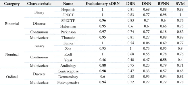
Table 3 presents the weighted mean recall of the algorithms. A recall rate is useful in determining the algorithm is not biased in recalling only the majority class of an imbalanced class dataset, rather also train and test instances from the minority class. An algorithm might have a high accuracy rate, but not a good recall rate. This can mean the algorithm only train and test instances from the majority class. For binomial datasets, Evolutionary DBN with bootstrap sampling possesses the highest recall rate when compared to other deep learning and machine learning algorithms. In this category, the recall rate for Evolutionary DBN with bootstrap sampling ranges from 0.95 to 1.0, which is very good as opposed to the recall rate from DBN that ranges from 0.6 to 0.83. For other algorithms, the lowest recall rate in a binomial category is BPNN for Parkinson dataset at 0.18, and the highest recall rate is SVM for SPECT dataset at 1.0. This shows that Evolutionary DBN with bootstrap sampling manages to learn and recall instances for prediction from both datasets despite its differences in attribute characteristic types and number of attributes, as shown in Table 1.
Table 3. Weighted Mean Recall of Algorithms
Category Characteristic Name Evolutionary sDBN DBN DNN BPNN SVM
Binomial Binary Hepatitis 1 0.81 0.68 0.88 0.88 SPECT 1 0.83 0.77 0.98 1 Discrete SPECTF 0.96 0.83 0.7 0.6 0.76 Haberman 0.95 0.6 0.6 0.66 0.73 Continuous Parkinson 0.97 0.74 0.77 0.18 0.82 Multivariate Thoracic 0.95 0.81 0.27 0.88 0.88 Nominal Binary Tumor 1 0.54 0.06 0.69 0.77 Zoo 0.95 1 0.73 0.95 0.9 Continuous Ecoli 1 0.68 0.55 0.78 0.76 Yeast 0.46 0.48 0.47 0.58 0.4 Multivariate Audiology 0.88 0.75 0.23 0.79 0.71 Ordinal Discrete Contraceptive 0.98 0.47 0.33 0.57 0.63 Dermatology 0.6 0.58 0.93 0.94 0.92 Multivariate Post-operative 0.94 0.72 0.27 0.72 0.78
For nominal datasets, Evolutionary DBN with bootstrap sampling achieved perfect recall rate of 1.0 for imbalanced class datasets, Tumor and Ecoli. Both imbalanced class datasets have binary and continuous numerical characteristics for their attributes respectively. When we compare the recall rate in each attribute category, Evolutionary DBN with bootstrap sampling has a high recall rate for binary attributes, which scored 1.0 and 0.95 for respective datasets. However, for continuous numerical attribute category, Evolutionary DBN with bootstrap sampling has a recall rate of 1.0 for Ecoli dataset, but only 0.46 for Yeast dataset. As mentioned previously in accuracy rate analysis and according to Table 1, both of the mentioned imbalanced class datasets are similar in attribute characteristics, data distribution, and the number of classes. Although the difference of the number of instances is staggering between the two imbalanced class datasets, it is unlikely that is the main factor for the underperformance of Evolutionary DBN with bootstrap sampling, considering the number of instances for Yeast dataset is similar to the number of instances for Contraceptive dataset. When compared the performance with other deep learning and machine learning algorithms, the highest recall rate is achieved by BPNN at 0.58, while the rest has a recall rate from 0.4 to 0.48. It is fair to conclude that the algorithms have difficulties in learning from this particular imbalanced class dataset.
As a conclusion for a nominal category, with exception to Yeast dataset, Evolutionary DBN with bootstrap sampling scored a high recall rate from 0.88 to 1.0 for the rest of imbalanced class datasets.
Although DBN manages to achieve a recall rate of 1.0 for Zoo dataset, its recall rate in other datasets is fairly low when compared to Evolutionary DBN with bootstrap sampling. Evolutionary DBN with bootstrap sampling manages to show an improvement of recall rate when compared to DBN, which means the algorithm is less biased when using the instances from both majority and minority classes in nominal type imbalanced class datasets.
For ordinal datasets, Evolutionary DBN with bootstrap sampling presents the highest recall rate for two imbalanced class datasets. As clarified previously in the accuracy rate analysis section, Evolutionary DBN with bootstrap sampling exhibits low recall rate for Dermatology dataset, despite there is an increment from DBN. This shows that the evolutionary and bootstrap sampling feature of the algorithm manages to improve the recall rate of DBN. However, the performance is relatively low when compared to other deep learning and machine learning algorithms. However, the inverse is shown for the other two imbalanced class datasets. For example, for Contraceptive datasets, Evolutionary DBN with bootstrap sampling exhibits not only the highest recall rate at 0.98, but the difference with the lowest recall rate of DNN at 0.33, is much more as contrast to the comparison between the highest recall rate for Dermatology dataset at 0.93 by DNN to 0.6 by Evolutionary DBN with bootstrap sampling. Based on the recall rate for an ordinal category, it can be concluded that Evolutionary DBN with bootstrap sampling manages to recall the instances for prediction and also minimize the partiality towards minority classes in the datasets.
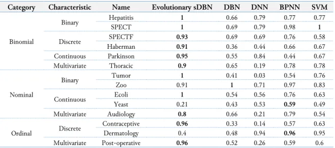
3.3.Weighted Mean Precision
Table 4 presents the weighted mean precision of the algorithms. Precision is a commonly used performance metric to determine the preciseness of an algorithm. A precision takes account the correctly classified from the actual classification. This measures the sensitivity of an algorithm. The closer its value to 1, the more precise it is. Consistent with accuracy rate and recall rate from Table 2 and Table 3, Evolutionary DBN with bootstrap sampling has the highest precision rate for imbalanced class datasets in a binomial category. However, the precision rate is smaller as compared to the recall rate from Table 2. This observation can conclude that the algorithm has more false positive (FP) compared to false negative (FN). For example, in Haberman dataset, “0” is labeled when the patient survived 5 years or longer after an operation for breast cancer and “1” is labeled if the patient died within 5 years. Since the FP is higher, it means the number of Types I Error is higher. The number of patients predicted to survive for 5 years or longer are wrongly classified, when they are actually dead within 5 years are higher, when compared to a smaller number of Type II Error where the number of patients predicted to be dead within 5 years are actually survived for 5 years or longer.
Table 4. Weighted Mean Precision of Algorithms
Category Characteristic Name Evolutionary sDBN DBN DNN BPNN SVM
Binomial Binary Hepatitis 1 0.66 0.79 0.77 0.77 SPECT 1 0.69 0.79 0.98 1 Discrete SPECTF 0.93 0.69 0.69 0.76 0.58 Haberman 0.91 0.36 0.44 0.66 0.67 Continuous Parkinson 0.95 0.55 0.84 0.44 0.67 Multivariate Thoracic 0.9 0.65 0.19 0.78 0.78 Nominal Binary Tumor 1 0.41 0.03 0.54 0.76 Zoo 0.91 1 0.71 0.97 0.83 Continuous Ecoli 1 0.54 0.56 0.76 0.63 Yeast 0.21 0.43 0.53 0.59 0.49 Multivariate Audiology 0.8 0.66 0.21 0.79 0.54 Ordinal Discrete Contraceptive 0.96 0.33 0.14 0.57 0.63 Dermatology 0.4 0.48 0.94 0.96 0.95 Multivariate Post-operative 0.96 0.52 0.26 0.59 0.6
In the nominal category, the precision result for all the algorithms is also consistent with the accuracy rate and recall rate. Similar to the performance of precision rate in a binomial category, the precision rate in the nominal category is a bit lower as compared to its recall rate. The precision rate for Evolutionary DBN with bootstrap sampling is high for all the imbalanced class datasets except for Yeast dataset. The range of precision rate for this category is from 0.03 to 1.0. Evolutionary DBN with bootstrap sampling manages to achieve precision rate from 0.8 to 1.0 for 4 out of 5 imbalanced class datasets.
In ordinal category, Evolutionary DBN with bootstrap sampling achieved the highest precision rate for 2 out of 3 imbalanced class datasets. However, for Post-operative dataset, the precision rate is higher than its recall rate. To conclude, the precision rate for Evolutionary DBN with bootstrap sampling is high as it scores from 0.8 to 1.0 except for 2 imbalanced class datasets in both nominal and ordinal categories, which rates at 0.21 and 0.4 respectively. This shows that Evolutionary DBN with bootstrap sampling algorithm is precise for binomial imbalanced class datasets, but for the multiclass category, the algorithm performs well but except for two imbalanced class datasets as shown in Table 4.
3.4.F1-score
F1-score is a good measure to decide how synchronized is our recall and precision values. An algorithm can have a good recall rate, but have low precision rate or vice versa. Therefore, it raises the question of whether the algorithm has a good performance. This is where F1-score is useful, as it takes into consideration both recall and precision rates and finds its harmonic value. Similar to recall and precision, as the F1-score is closer to value 1; the algorithm has an agreeable recall and precision rates. In binomial category, the F1-score achieved by Evolutionary DBN with bootstrap sampling is from 0.92 to 1.0. These score presents an improvement as compared to F1-score achieved by DBN, which is from0.45 to 0.76. From Table 5, SVM has a score between 0.64 to 1.0, which is quite stable as compared to DNN and BPNN. As mentioned previously in accuracy rate, the SVM structure makes it easy to learn and predict from imbalanced class datasets in the binomial category. Considering the structure of Evolutionary DBN with bootstrap sampling has similar node structure as DBN, DNN, and BPNN, this shows a huge increment of performance in this category. The F1-score observation deduces that Evolutionary DBN with bootstrap sampling has high accuracy as well as high recall and precision.
Table 5. F1-score of Algorithms
Category Characteristic Name Evolutionary sDBN DBN DNN BPNN SVM
Binomial Binary Hepatitis 1 0.73 0.46 0.82 0.82 SPECT 1 0.76 0.74 0.98 1 Discrete SPECTF 0.94 0.76 0.69 0.64 0.66 Haberman 0.93 0.45 0.49 0.66 0.64 Continuous Parkinson 0.96 0.63 0.8 0.1 0.74 Multivariate Thoracic 0.92 0.72 0.25 0.83 0.83 Nominal Binary Tumor 1 0.46 0.03 0.59 0.74 Zoo 0.93 1 0.72 0.95 0.86 Continuous Ecoli 1 0.6 0.56 0.75 0.69 Yeast 0.29 0.44 0.49 0.56 0.33 Multivariate Audiology 0.84 0.7 0.22 0.73 0.61 Ordinal Discrete Contraceptive 0.97 0.37 0.93 0.57 0.63 Dermatology 0.47 0.51 0.1 0.95 0.91 Multivariate Post-operative 0.95 0.61 0.26 0.65 0.68
As for nominal category, except Yeast dataset, the F1-score achieved by Evolutionary DBN with bootstrap sampling is from 0.84 to 1.0. As we can see from Table 2 and Table 3, although the decrement of accuracy and recall rate between Evolutionary DBN with bootstrap sampling and DBN seems small, due to the low precision value of Evolutionary DBN with bootstrap sampling for the mentioned
imbalanced class dataset, the F1-score difference between the algorithm and DBN is large, which is 0.29 and 0.44 respectively. It can be assumed that Evolutionary DBN with bootstrap sampling cannot learn from the dataset. However, when compared to other deep learning and machine learning algorithms, Yeast dataset only managed to receive the highest F1-score performance at 0.56 by BPNN. This is very low especially when we contrast to other imbalanced class datasets in the nominal category, the highest F1-score can be achieved from 0.84 to 1.0. Evolutionary DBN with bootstrap sampling achieves all these high F1-scores. Therefore, despite the previous assumption, it can also be concluded that Yeast dataset has a complex feature that is difficult for other deep learning and machine learning algorithms to learn from as well.
Nevertheless, for the rest of imbalanced class datasets in the nominal category, it can be inferred that Evolutionary DBN with bootstrap sampling’s performance for accuracy, recall and precision is established based on its high performance of F1-score. In ordinal category, Evolutionary DBN with bootstrap sampling has the highest F1-score for 2 out of 3 imbalanced class datasets. It is consistent with its performance for accuracy, recall and precision rates in Table 2, Table 3, and Table 4. In both datasets, Evolutionary DBN with bootstrap sampling shows an improvement when compared to DBN. As for Dermatology dataset, the F1-score is affected by the low precision value in Table 4. Despite the improved accuracy and recall rates of Evolutionary DBN with bootstrap sampling when compared to DBN, the result shows that the algorithm is not as precise as reflected in other metrics.
4.
Conclusion
Based on the result analyses derived from the performance metrics, Evolutionary DBN with bootstrap sampling outperforms DBN and other deep learning and machine learning algorithms for imbalanced class datasets in a binomial category. However, for multiclass categories, nominal and ordinal, the result is mixed. For example, in a nominal category, Evolutionary DBN with bootstrap sampling outperforms DBN and other deep learning and machine learning algorithms for 3 out of 5 imbalanced class datasets. In Zoo dataset, the result for Evolutionary DBN with bootstrap sampling dropped as compared to when DBN is used. Although Evolutionary DBN with bootstrap sampling has fairly high performance, it is likely that the addendum structure of Evolutionary algorithm and bootstrap sampling to the DBN component made the learning from the specific dataset made the weight calculations in the algorithm too complicated when such dataset is used. In ordinal category, Evolutionary DBN with bootstrap sampling performs well for 2 out of 3 imbalanced class datasets. In Dermatology dataset, Evolutionary DBN with bootstrap sampling showed an increment of accuracy and recall performance when compared with DBN, in contrast to its performance for Zoo dataset in a nominal category. Despite the increased performance in both of the metrics, both Evolutionary DBN with bootstrap sampling and DBN still have the lowest performance in this dataset as compared to other deep learning and machine learning algorithms. It is likely that the structure of both algorithms are not suitable for this type of dataset considering DNN and BPNN, which has similar algorithm structure and calculation manage to achieve the two highest performance for this particular dataset. It can be concluded that for multiclass imbalanced class datasets, Evolutionary DBN with bootstrap sampling performs fairly well even if the result is not as solid as when binomial imbalanced class datasets are used. Another observation that can be made is that Evolutionary DBN with bootstrap sampling performs well on imbalanced class datasets that posses multivariate attributes type in all the categories.
Acknowledgment
This study is financially supported by a grant from the Ministry of Higher Education Malaysia: Fundamental Research Grant Scheme (FRGS-19-074-0682).
References
[1] G. M. Weiss and F. Provost, “The effect of class distribution on classifier learning: an empirical study,” Technical Report ML-TR-44, 2001, available at: https://rucore.libraries.rutgers.edu/rutgers-lib/59563/ PDF/1/play/.
[2] J. Zhai, S. Zhang, and C. Wang, “The classification of imbalanced large data sets based on MapReduce and ensemble of ELM classifiers,” Int. J. Mach. Learn. Cybern., vol. 8, no. 3, pp. 1009–1017, Jun. 2017, doi:
10.1007/s13042-015-0478-7.
[3] H. Han, W.-Y. Wang, and B.-H. Mao, “Borderline-SMOTE: A New Over-Sampling Method in Imbalanced Data Sets Learning,” 2005, pp. 878–887, doi: 10.1007/11538059_91.
[4] Y. Liu, X. Yu, J. X. Huang, and A. An, “Combining integrated sampling with SVM ensembles for learning from imbalanced datasets,” Inf. Process. Manag., vol. 47, no. 4, pp. 617–631, Jul. 2011, doi:
10.1016/j.ipm.2010.11.007.
[5] T. Wang, D. J. Wu, A. Coates, and A. Y. Ng, “End-to-end text recognition with convolutional neural networks,” in Proceedings of the 21st International Conference on Pattern Recognition (ICPR2012), 2012, pp. 3304–3308, available at: https://ieeexplore.ieee.org/abstract/document/6460871.
[6] A. Mohamed, G. E. Dahl, and G. Hinton, “Acoustic Modeling Using Deep Belief Networks,” IEEE Trans.
Audio. Speech. Lang. Processing, vol. 20, no. 1, pp. 14–22, Jan. 2012, doi: 10.1109/TASL.2011.2109382. [7] D. Le and E. M. Provost, “Emotion recognition from spontaneous speech using Hidden Markov models
with deep belief networks,” in 2013 IEEE Workshop on Automatic Speech Recognition and Understanding, 2013, pp. 216–221, doi: 10.1109/ASRU.2013.6707732.
[8] A. Mohamed, G. Hinton, and G. Penn, “Understanding how Deep Belief Networks perform acoustic modelling,” in 2012 IEEE International Conference on Acoustics, Speech and Signal Processing (ICASSP), 2012, pp. 4273–4276, doi: 10.1109/ICASSP.2012.6288863.
[9] P. Hensman and D. Masko, “The impact of imbalanced training data for convolutional neural networks,”
Degree Proj. Comput. Sci. KTH R. Inst. Technol., 2015, available at: https://www.kth.se/social/files/588617
ebf2765401cfcc478c/PHensmanDMasko_dkand15.pdf.
[10] Y. Yan, M. Chen, M.-L. Shyu, and S.-C. Chen, “Deep Learning for Imbalanced Multimedia Data Classification,” in 2015 IEEE International Symposium on Multimedia (ISM), 2015, pp. 483–488, doi:
10.1109/ISM.2015.126.
[11] A. Fernández, S. García, and F. Herrera, “Addressing the Classification with Imbalanced Data: Open Problems and New Challenges on Class Distribution,” 2011, pp. 1–10, doi: 10.1007/978-3-642-21219-2_1. [12] W. Liu and S. Chawla, “Class Confidence Weighted kNN Algorithms for Imbalanced Data Sets,” 2011, pp.
345–356, doi: 10.1007/978-3-642-20847-8_29.
[13] K. Swersky, B. Chen, B. Marlin, and N. de Freitas, “A tutorial on stochastic approximation algorithms for training Restricted Boltzmann Machines and Deep Belief Nets,” in 2010 Information Theory and Applications
Workshop (ITA), 2010, pp. 1–10, doi: 10.1109/ITA.2010.5454138.
[14] N. V. Chawla, N. Japkowicz, and A. Kotcz, “Editorial: special issue on learning from imbalanced data sets,”
ACM SIGKDD Explor. Newsl., vol. 6, no. 1, p. 1, Jun. 2004, doi: 10.1145/1007730.1007733.
[15] O. A. John, A. Adebayo, and O. Samuel, “Effect of Feature Ranking on the Detection of Credit Card Fraud: Comparative Evaluation of Four Techniques,” I-Manager’S J. Pattern Recognit., Vol. 5, No. 3, P. 10, 2018, doi: 10.26634/JPR.5.3.15676.
[16] J. Berry, I. Fasel, L. Fadiga, and D. Archangeli, “Entropy coding for training deep belief networks with imbalanced and unlabeled data,” J. Acoust. Soc. Am., vol. 131, no. 4, pp. 3235–3235, Apr. 2012, doi:
10.1121/1.4708066.
[17] O. Ghahabi and J. Hernando, “Deep belief networks for i-vector based speaker recognition,” in 2014 IEEE
International Conference on Acoustics, Speech and Signal Processing (ICASSP), 2014, pp. 1700–1704, doi:
10.1109/ICASSP.2014.6853888.
[18] M. Rosca, “Networks with emotions: An investigation into deep belief nets and emotion recognition,” Imperial College London, 2014, available at: http://elarosca.net/report.pdf.
[19] F. Megumi, A. Yamashita, M. Kawato, and H. Imamizu, “Functional MRI neurofeedback training on connectivity between two regions induces long-lasting changes in intrinsic functional network,” Front. Hum.
[20] Z. Sun, H. Sun, and J. Zhang, “Multistep Wind Speed and Wind Power Prediction Based on a Predictive Deep Belief Network and an Optimized Random Forest,” Math. Probl. Eng., vol. 2018, pp. 1–15, Jul. 2018, doi: 10.1155/2018/6231745.
[21] S. Dieleman, P. Brakel, and B. Schrauwen, “Audio-based music classification with a pretrained convolutional network,” in 12th International Society for Music Information Retrieval Conference (ISMIR-2011), 2011, pp. 669–674, available at: Google Scholar.
[22] H. Lee, R. Grosse, R. Ranganath, and A. Y. Ng, “Unsupervised learning of hierarchical representations with convolutional deep belief networks,” Commun. ACM, vol. 54, no. 10, pp. 95–103, 2011, doi:
10.1145/2001269.2001295.
[23] W.-L. Zheng, J.-Y. Zhu, Y. Peng, and B.-L. Lu, “EEG-based emotion classification using deep belief networks,” in 2014 IEEE International Conference on Multimedia and Expo (ICME), 2014, pp. 1–6, doi:
10.1109/ICME.2014.6890166.
[24] K. Terusaki and V. Stigliani, “Emotion Detection using Deep Belief Networks,” 2014, available at:
https://pdfs.semanticscholar.org/e9bf/a43c8008632559ec5320420c6bfa438766c7.pdf.
[25] C. Huang, W. Gong, W. Fu, and D. Feng, “A Research of Speech Emotion Recognition Based on Deep Belief Network and SVM,” Math. Probl. Eng., vol. 2014, pp. 1–7, 2014, doi: 10.1155/2014/749604. [26] G. E. Hinton, “Training Products of Experts by Minimizing Contrastive Divergence,” Neural Comput., vol.
14, no. 8, pp. 1771–1800, Aug. 2002, doi: 10.1162/089976602760128018.
[27] T. Jo and J.-H. Lee, “Latent Keyphrase Extraction Using Deep Belief Networks,” Int. J. Fuzzy Log. Intell.
Syst., vol. 15, no. 3, pp. 153–158, Sep. 2015, doi: 10.5391/IJFIS.2015.15.3.153.
[28] A. A. Amri, A. R. Ismail, and A. Ahmad Zarir, “Convolutional Neural Networks and Deep Belief Networks for Analysing Imbalanced Class Issue in Handwritten Dataset,” Int. J. Adv. Sci. Eng. Inf. Technol., vol. 7, no. 6, p. 2302, Dec. 2017, doi: 10.18517/ijaseit.7.6.2632.
[29] Z. Lanbouri and S. Achchab, “A hybrid Deep belief network approach for Financial distress prediction,” in
2015 10th International Conference on Intelligent Systems: Theories and Applications (SITA), 2015, pp. 1–6, doi:
10.1109/SITA.2015.7358416.
[30] D. Kuang and L. He, “Classification on ADHD with Deep Learning,” in 2014 International Conference on
Cloud Computing and Big Data, 2014, pp. 27–32, doi: 10.1109/CCBD.2014.42.
[31] S. Ganguly and D. Samajpati, “Distributed Generation Allocation on Radial Distribution Networks Under Uncertainties of Load and Generation Using Genetic Algorithm,” IEEE Trans. Sustain. Energy, vol. 6, no. 3, pp. 688–697, Jul. 2015, doi: 10.1109/TSTE.2015.2406915.
[32] M. Qiu, Z. Ming, J. Li, K. Gai, and Z. Zong, “Phase-Change Memory Optimization for Green Cloud with Genetic Algorithm,” IEEE Trans. Comput., vol. 64, no. 12, pp. 3528–3540, Dec. 2015, doi:
10.1109/TC.2015.2409857.
[33] P. Ghamisi and J. A. Benediktsson, “Feature selection based on hybridization of genetic algorithm and particle swarm optimization,” IEEE Geosci. Remote Sens. Lett., vol. 12, no. 2, pp. 309–313, 2014, doi:
10.1109/LGRS.2014.2337320.
[34] D. Liu, D. Niu, H. Wang, and L. Fan, “Short-term wind speed forecasting using wavelet transform and support vector machines optimized by genetic algorithm,” Renew. Energy, vol. 62, pp. 592–597, Feb. 2014, doi: 10.1016/j.renene.2013.08.011.
[35] M. Jamshidi, M. Ghaedi, K. Dashtian, S. Hajati, and A. Bazrafshan, “Ultrasound-assisted removal of Al 3+ ions and Alizarin red S by activated carbon engrafted with Ag nanoparticles: central composite design and genetic algorithm optimization,” RSC Adv., vol. 5, no. 73, pp. 59522–59532, 2015, doi:
10.1039/C5RA10981G.
[36] M. N. Haque, N. Noman, R. Berretta, and P. Moscato, “Heterogeneous Ensemble Combination Search Using Genetic Algorithm for Class Imbalanced Data Classification,” PLoS One, vol. 11, no. 1, p. e0146116, Jan. 2016, doi: 10.1371/journal.pone.0146116.
[37] M. Elhoseny, X. Yuan, Z. Yu, C. Mao, H. K. El-Minir, and A. M. Riad, “Balancing Energy Consumption in Heterogeneous Wireless Sensor Networks Using Genetic Algorithm,” IEEE Commun. Lett., vol. 19, no. 12, pp. 2194–2197, Dec. 2015, doi: 10.1109/LCOMM.2014.2381226.
[38] S. Oreski and G. Oreski, “Genetic algorithm-based heuristic for feature selection in credit risk assessment,”
Expert Syst. Appl., vol. 41, no. 4, pp. 2052–2064, Mar. 2014, doi: 10.1016/j.eswa.2013.09.004.
[39] M. J. Neath, A. K. Swain, U. K. Madawala, and D. J. Thrimawithana, “An Optimal PID Controller for a Bidirectional Inductive Power Transfer System Using Multiobjective Genetic Algorithm,” IEEE Trans.
Power Electron., vol. 29, no. 3, pp. 1523–1531, Mar. 2014, doi: 10.1109/TPEL.2013.2262953.
[40] H. Assodiky, I. Syarif, and T. Badriyah, “Deep learning algorithm for arrhythmia detection,” in 2017
International Electronics Symposium on Knowledge Creation and Intelligent Computing (IES-KCIC), 2017, pp.
26–32, doi: 10.1109/KCIC.2017.8228452.
[41] E. Inanlo and J. M. Zadeh, “Social Networks Classification using DBN Neural Network based on Genetic Algorithm,” Int. J. Innov. Adv. Comput. Sci., vol. 5, no. 11, pp. 7–-10, 2016, available at: Google Scholar. [42] A. R. Deshmukh and S. P. Akarte, “Classification of Imbalanced Medical Data Efficiently Using Multiclass
SVM and Genetic Algorithm,” Int. J. Comput. Sci. Mob. Comput., vol. 5, no. 1, pp. 144–-147, 2016, available at: Google Scholar.
[43] T. Perry, M. Bader-El-Den, and S. Cooper, “Imbalanced classification using genetically optimized cost sensitive classifiers,” in 2015 IEEE Congress on Evolutionary Computation (CEC), 2015, pp. 680–687, doi:
10.1109/CEC.2015.7256956.
[44] E. Asadi, M. G. da Silva, C. H. Antunes, L. Dias, and L. Glicksman, “Multi-objective optimization for building retrofit: A model using genetic algorithm and artificial neural network and an application,” Energy
Build., vol. 81, pp. 444–456, Oct. 2014, doi: 10.1016/j.enbuild.2014.06.009.
[45] Q. Gu, L. Zhu, and Z. Cai, “Evaluation measures of the classification performance of imbalanced data sets,” in International symposium on intelligence computation and applications, 2009, pp. 461–471, doi: 10.1007/978-3-642-04962-0_53.
[46] C. Zhang, K. C. Tan, H. Li, and G. S. Hong, “A cost-sensitive deep belief network for imbalanced classification,” IEEE Trans. neural networks Learn. Syst., vol. 30, no. 1, pp. 109–122, 2018, doi:
10.1109/TNNLS.2018.2832648.
[47] S. Boughorbel, F. Jarray, and M. El-Anbari, “Optimal classifier for imbalanced data using Matthews Correlation Coefficient metric,” PLoS One, vol. 12, no. 6, p. e0177678, Jun. 2017, doi:
10.1371/journal.pone.0177678.
[48] V. López, A. Fernández, S. García, V. Palade, and F. Herrera, “An insight into classification with imbalanced data: Empirical results and current trends on using data intrinsic characteristics,” Inf. Sci. (Ny)., vol. 250, pp. 113–141, Nov. 2013, doi: 10.1016/j.ins.2013.07.007.