Chapter 4
Design of Experiments
4.1 Introduction
In Chapter 3 we have considered the location of the data points fixed and studied how to pass a good response surface through the given data. However, the choice of points where experiments (whether numerical or physical) are performed has very large effect on the accuracy of the response surface, and in this chapter we will explore methods for selecting a good set of points for carrying out experiments. The selection of these points is known as design of experiments.
Design of experiments is inherently a multi-objective optimization problem. We would like to select points so that we maximize the accuracy of the information that we get from the experiments. We usually also would like to minimize the number of experiments, because these are expensive. In some cases the objective of the experiments is to estimate some physical characteristics, and in these cases, we would like to maximize the accuracy of these characteristics. However, in the design applications, which are of primary interest to us, we would like to construct a response surface that could be used to predict the performance of other designs. In this case, our primary goal is to choose the points for the experiments so as to maximize the predictive capability of the model.
A lot of work has been done on experimental designs in regular design domains. Such domains occur when each design variable is bounded by simple lower and upper limits, so that the design domain is box like. Occasionally, spherical domains are also considered. Sometimes each design variable can take only two or three values, often called levels. These levels are termed low, nominal and high. In other cases, the design space is approximately box like, but it is possible to carry experiments with the design variables taking values outside the box for the purpose of improving the properties of the response surface. In the next section we will summarize briefly some of the properties of experimental design in box-like domains, and present some of the more popular experimental designs in such domains.
For design optimization, however, it is common for us to try and create response surfaces in irregularly shaped domains. In that case, we have to create our own experimental design. Section 4.3 will discuss several techniques available for finding good designs in an irregular shaped domain.
4.2 Design of Experiments in Boxlike Domains
In this case the region of interest is defined by simple lower and upper limits on each of the design variables
,
,....,
1
,
'n
i
x
x
x
il
i
iu
(4.2.1)where
x
il, andx
iuare the lower and upper limits, respectively, on the design variablex
i'. The prime indicates that the design variable has not been normalized. For convenience we normalize the design variable as,
2
' il iu in il i ix
x
x
x
x
x
(4.2.2)The normalized variables are then all bound in the cube
,
1
1
x
i (4.2.3)4.2.1 Interpolation, extrapolation and prediction variance
The simplest experimental design for the cube is one experiment at each one of the
2
nvertices (Matlab ff2n). This design is called a 2-level full factorial design, where the word `factorial' refers to 'factor', a synonym for design variable, rather than the factorial function. For a small number of design variables,2
nmay be a manageable number of experiments. More general full-factorial designs may have different number of levels in different directions (Matlab fullfact). However, for larger values of n, we usually cannotafford even the two-level full factorial design. For example, forn10, we
get
2
n
1024
.
For high values of n we may consider fractional factorial designs, which do not include all the vertices (see Matlab’s fracfact).If we want to fit a linear polynomial to the data, it certainly appears that we will not need anywhere near
2
npoints for a good fit. For example, for n = 10, we have 11 coefficients to fit, and using 1024 experiments to fit these 11 coefficients may appear excessive even if we could afford that many experiments. However, with fewer experiments we lose an important property of using the response surface as aninterpolation tool rather than as a tool for extrapolation. To understand that we will first define what we mean by interpolation and extrapolation.
Intuitively, we say that our response surface will interpolate the data at a point, if that point is `completely surrounded' by data points. In one dimensional space, this means that there is a point to the right of the interpolated point, as well as a point to the left of it. In two-dimensional space we would like the point to be surrounded by at least 3 points, so that it falls inside the triangle defined by these 3 points. Similarly, in three-dimensional space, we would like the point to be surrounded by at least 4 points, that is
tetrahedron; a shape in n dimensional space defined by n+ 1 linearly independent points.
Given a set of n + 1 points in n-dimensional space,
x x
1,
2,...,
x
n1, the simplex defined by these points includes all the points that can be obtained by a convex sum of these points. That is, it includes any point x, which may be written as1 1
,
n i i i
x
x
(4.2.4) With
1 1,
1
n i i
and
i
0
,
i
1
,
,
,
,
,
,
n
1
,
(4.2.5)Given a set of
n
ydata points, the set of points where the response surface performs interpolation is the union of all of these simplexes, which is also called the convex hull of the data points.One measure that we can use to estimate the loss of prediction accuracy incurred when we use extrapolation is the prediction variance. Recall that the linear regression model that we use may be written as
1
ˆ
( ),
n i i iy
b
x
(4.2.6)Defining the vector
x
( )m by ( )( ),
mi i
x
x
(4.2.7)we can write Eq. 4.2.6 as ( )
ˆ
m T,
y
x
b
(4.2.8)With noise in the data, b has some randomness to it, while
x
( )m is deterministic. Using Eq. 3.2.29, it is easy to show that the variance (square of the standard deviation) ofy
ˆ
is given as
1 ( ) ( ) 2 ( ) ( )ˆ
[ ( )]
m T b m m T T m,
Var y
x
x
x
x
X X
x
(4.2.9) with the standard deviation ofy x
ˆ( )
being the square root of this expression. If we use the estimate
ˆ
instead of
, we get the standard errors
yofy
ˆ
1( ) ( )
ˆ
m T T my
s
x
X X
x
(4.2.10)The standard error gives us an estimate of the sensitivity of the response surface prediction at different points to errors in the data. We would like to select points so as to make this error as small as possible everywhere in the domain where we would like to estimate the response.
Intuitively, it appears that this would be helped if the standard error did not vary much from one point to another. This property is called stability. The following example demonstrates the effect of using extrapolation on the stability of the standard error.
Example 4.2.1
Consider the problem of fitting a linear polynomial
y
b
1
b
2x
1
b
3x
2to data in the square1 1
, 1
1 1 2
x x . Compare the maximum value of the prediction variance for two cases; (a) Full factorial design (points at all 4 vertices). (b) A fractional design including 3 vertices, obtained by omitting the vertex (1, 1).
Full factorial design: We number the points as
x
1T
1
,
1
,
x
T2
1
,
1
,
x
3T
1
,
1
,
x
T4
1
,
1
. For this case we have1 1 1
1 0 0
1 1 1
,
4 0 1 0
1 1 1
0 0 1
1 1 1
TX
X X
, (4.2.11) Also 2 1 ) ( 1 x x xm ,x
(m)T
X
TX
1x
(m)
0
.
25
(
1
x
12
x
22),
(4.2.12) Using Eq. 4.2.10, we see that the standard error of the response varies betweensy
ˆ 2at theorigin and
s
y
3
ˆ
2
at the vertices. This case represents a fairly stable variation of the error of only3
between the smallest and highest value in the domain of interest.Fractional factorial design: This time we have
, 3 1 1 1 3 1 1 1 3 , 1 1 1 1 1 1 1 1 1 X X X T (4.2.13) and
1 2 1 1 0.25 1 2 1 , 1 1 2 T X X
1
( ) ( ) 2 2 1 2 1 2 1 20.5 1
,
m T T mX X
x
x
x
x
x x
x
x
(4.2.14)At the origin the standard error is stillsy
ˆ 2, at the three vertices we getsy
ˆ. This is expected, as with only 3 data points the response surface passes through the data, so that the error at the data points should be measurement error. However, at the fourth vertex (1,1), where the response surface represents extrapolation, we getsy 3
ˆ. By setting the derivatives of the prediction error to zero, we easily find that the minimum error is at the centroid of the three data points, at(1 3,13). At the centroidsy
ˆ 3.Now the ratio between the smallest and highest standard errors is 5.2, with the highest errors in the region of extrapolation.It can be checked that when we use a full factorial design for a linear polynomial in n variables, we get
X
TX
2
nI
,
, where I is a unit of order n+ 1. This will give us2 2 2 1 2 2 ˆ 1 .... 2 y n n s
x x x (4.2.15)so that the maximum prediction error (achieved at any vertex) is
ˆ
n
1 / 2 .
n That is the quality of the fit becomes very good with increasing n. This reflects the fact that we use2
npoints to calculate n + 1 coefficients, so that we average out the effect of noise. This estimate is misleading in actual situations, because rarely do we have a true linear model. When the response we measure is not linear, we will have modeling errors, also called bias errors which are not averaged out.If on the other hand, we take only enough measurements to calculate the coefficients, that is a saturated design with n + 1 coefficients, the error gets progressively bigger, because the portion of design space covered by the simplex containing the data points becomes progressively smaller. For example, for Example 4.2.1 the three points used for the saturated design form a triangle covering half of the design domain. For a three dimensional cube, 4 vertices will span a tetrahedron with a volume of one sixth of the volume of the enclosing cube. For the n dimensional case, the full-factorial design is the vertices of a cube of volume
2
n, while n + 1 vertices obtained by perturbing one variable at a time from one vertex span a simplex of volume2
nn
!.
For example, for three dimensions, the maximum prediction error with a full-factorial design is0
.
5
, while the maximum prediction error for the saturated 4-point fractional factorial design is7
(Exercise 1).4.2.2 Designs for linear response surfaces
For fitting linear response surfaces, we typically use designs with only two levels for each design variable, and the most popular fractional designs are the so called
orthogonal designs. An orthogonal design is one where the matrix XTX is diagonal, and the popularity of these designs is partly based on the following theorem (see Myers and Montgomery, 1995 p. 284):
For the first-order model (linear polynomial) and a fixed sample size. If all variables lie between -1 and 1, then the variance of the coefficients is minimized if the design is orthogonal, and all the variables are at their outer positive or negative limits (i.e., -1 or +1).
It is easy to check that the full factorial design is orthogonal, but it is not trivial to produce orthogonal designs with smaller number of measurements. Various orthogonal designs can be found in books on design of experiments (see Myers and Montgomery, 1995). To demonstrate the beneficial properties of orthogonal designs we will consider the two-dimensional case that we have studied in the previous example. In that example we fitted a two-variable linear polynomial first with a full factorial design and then with only 3 points. Fitting a linear polynomial in n variables on the basis of n+1 points requires the points to be linearly independent, so that they form a simplex. There is no redundancy in the design, in that the number of points is equal to the number of coefficients, and this is called a saturated design. In order to get an orthogonal design in this case, we have to give up on having the variables be only at the
1
levels, and instead opt for a perfect simplex, with the distance between all points being the same.Example 4.2.2
Consider the equilateral triangle which results in a scalar matrix (a scalar matrix is a scalar multiple of the unit matrix)
X
TX
. It includes the points ( 3 2,1 2), ( 3 2,1 2), (0, 2). Check for the stability of the prediction variance and its maximum value in the unit square for the linear modely
b
1
b
2x
1
b
3x
2.We have 2 0 1 2 1 2 3 1 2 1 -2 3 1 X , 3 0 0 0 3 0 0 0 3 X XT . (4.2.16) Also
1
( ) ( ) ( ) 2 2 1 1 2 2 1 1 , 1 . 3 m m T T m x X X x x x x x x (4.2.17)Using Eq. 4.2.10, we see that the standard error of the response varies between sy
ˆ 3at the origin ands
y
ˆ
at the vertices. This is an improvement, both in terms of stability and maximum standard error as compared to using 3 vertices of the unit square. However, this has come at the price of doing the measurements outside the unit square. As we will see later, this reduces the variance error, but increases the so called bias error. Bias error is the error introduced when the model that we try to fit is different from the true function. For example, if the model is linear and the true function is quadratic, the simplex model that we have used in this example is likely to increase the error rather than decrease it.4.2.3 Designs for quadratic response surfaces
Quadratic polynomials in n variables have (n+1)(n+2)/2 coefficients. To fit quadratic response surfaces we need at least that many points, and at least three levels for each design variable. For n > 3 it is possible to have the requisite number of points with only two levels. For example, a quadratic polynomial in 4 variables has 15 coefficients, and a full factorial design in two levels has 16 points. However, if we let only one design variable vary at a time, we can easily check that we are left with 3 coefficients and we need three different levels of that design variable.
We can use a full-factorial 3-level design for the quadratic response surface, and this design will have
3
npoints. In most cases we cannot afford such designs even for fairly small values of n. For example, for n = 6, we require3
6
729
experiments. A popular compromise which reduces the number of experiments to close to the 2-level full factorial design is the central composite design (CCD) (Matlab ccdesign).The central composite design is composed of the
2
npoints of the full-factorial two-level design, with all the variables at their extremes, plus a number of repetitionsn
cof the nominal design, plus the 2n points obtained by changing one design variable at a time by an amount
.Figures 4.1 and 4.2 show the central composite design for n = 2 and n = 3. The value of
chosen in the figures are such that all the points outside the origin are of the same distance from the origin, so that we have a spherical design. This placement of the points is at the higher end of the typical choice for
. A more popular choice is based on the concept of rotatability. The property of rotatability requires that the prediction variance be dependent only on the distance from the origin and not on the orientation with respect to the coordinate axes.It can be shown that for the central composite design the rotatability requirement will be satisfied for 4
2
n
(4.2.18)This equation gives
2for n = 2, which is the same as the spherical design,however, for n = 3 we get
1.682, which is slightly smaller than3
.With either a spherical design or a rotatable one, we find that we need a number of replicate center points (points at the origin) to obtain good prediction variance stability. Figures 4.3 and 4.4 show contours of prediction variance with one central point and five central points, respectively. It is obvious that the stability of the latter is much better than the former. This need of central points with rotatable central composite designs is a possible problem with numerical experiments that give exactly the same answer when the experiment is repeated at the same point. Fortunately, however, with
1there is no need for repeated central points. The case of
1, which is called the face centered central composite design (FCCCD), is very attractive in a lot of applications, because it does not require using any other levels except (-1,0,1). Figure 4.5 shows contours of the prediction variance for the unit square with a single central point. It is seen that while theFor high dimensional spaces, the central composite design is no longer practical, because the number of points increases too fast. One possible solution is to keep the 2n runs which perturb a single variable, but to have an fractional factorial design to replace the
2
nvertices. However, while the number of vertices increases as2
n, the number of polynomial coefficients increases as (n + 1)(n + 2)/2. Consequently, the type of fractional design used has to be modified as n increases. Instead there is a block design (Matlab bbdesign), first introduced by Box and Behnken (1960), where the number of experiments increases at the same rate as the number of polynomial coefficients. The two-variable block design is based on perturbing only two variables from the nominal value. That is, at each point, we have a pair (I, j), such hatx
i
1
,
x
j
1
,
andx
k
0
forall
k
i
,
k
j
. The two variables are perturbed in all four combination of
1
. For example, for n = 3 (the lowest dimension for which this design makes sense) we will have the following design points3 2 1
x
x
x
-1 -1 0 -1 1 0 1 -1 0 1 1 0 -1 0 -1 -1 0 1 (4.2.19) 1 0 -1 1 0 1 0 -1 -1 0 -1 1 0 1 -1 0 1 1 0 0 0where the last point is the central point, which may be repeated. Figure 4.6 shows this design. For the general case, we can select 2 variables out ofninn(n1) 2ways. For each such combination of two variables we have four design points, with each one of the variables taking the values of
1
. The total number of points in this block design isn
c
2
n
(
n
1
)
. For large values ofnthis tends asymptotically to 4 times larger than thenumber of coefficients that we need to fit. However, this happens for very large values of n. For example, for n = 10 the number of coefficients is 66, while the number of points in the block design with one center point is 181 (for comparison, the number of points in the central composite design is 1045).
.
Block designs are spherical, in that all the points are at the same distance from the origin. For example, all the two-variable block design points are at a distance of 2from the origin. For large values ofn, this distance can be much smaller than the distance of the vertices (which is
n
). Therefore, extrapolating to the vertices on the basis of the block design may be risky.4.3 Optimal Point Selection
The special experimental designs that we considered so far, as well as other experimental designs available in the literature will satisfy our needs most of the time when we have a box-like domain. Often, however, we will not operate in a box-like domain because of various design constraints. In fact, it is desirable to invoke as many constraints as we can to reduce the volume of the design domain, because this typically increases the accuracy of the response surface. With an irregular design domain, the standard experimental designs are of no use to us. In fact, even with a box-like domain we may want to perform a number of experiments that does not correspond to any of the standard designs. In these cases we have to create our own experimental design, that is select an optimum set of design points.
4.3.1 Minimum variance designs
The common approach to optimum point selection treats it as a combinatorial problem. We start by creating a pool of candidate points where we could possibly evaluate the response. We will assume that we can afford
n
yevaluations of the design, so that out of the pool we would like to select the `best' ny points.There are various criteria as to what is the best set of points, and the most popular ones attempt to select the points so as to minimize the variance of the coefficients of the response surface. A key to that variance is the moment matrix
y T
n
X
X
M
(4.3.1)The determinant of the moment matrix
T n y X X M n (4.3.2)
can be shown to be directly related to confidence region of the coefficients of the response surface (a confidence region for a coefficient is the region where the coefficient will lie with a given probability). In fact, it is inversely proportional to the square of the volume of the confidence region of the coefficients. So maximizing the determinant increases our confidence in the coefficients. This criterion is called D-optimality, and it is implemented in several software packages.
Finding the D-optimal set of points from a given set of points is often a difficult combinatorial problem. For example, if we need to find 10 D-optimal points out of 50, we
10
set, and usually settle on a suboptimal but good set. Some solution algorithms are based on replacing one point at a time and taking advantage of inexpensive expressions for updating the determinant when one points is changed. Genetic algorithms have also been used to find a good design based on D-optimality.
Matlab has several functions that can be used for generating D-optimal designs. For box-like domain and linear and quadratic polynomials, one can use cordexch (name comes from using a coordinate exchange algorithm for searching for the D-optimal design).
Example 4.3.1:
--- We want to fit a quadratic polynomial in 2 variables (6 coefficients) and we want to see the effect of the number of points on the design and the determinant of the moment matrix. Using cordexch we start with the default 3 levels and compare using the minimum number of six points to using 10 points.
With six points: >> ny=6;nbeta=6; >> [dce,x]=cordexch(2,ny,'quadratic'); >> dce' ans = 1 1 -1 -1 0 1 -1 1 1 -1 -1 0 >> det(x'*x)/ny^nbeta ans = 0.0055 With 12 points: >> ny=12; >> [dce,x]=cordexch(2,ny,'quadratic'); >> dce' ans = -1 1 -1 0 1 0 1 -1 1 0 -1 1 1 -1 -1 -1 1 1 -1 -1 0 0 0 1 >> det(x'*x)/ny^nbeta ans =0.0102
We note that the points are selected on the boundary and that for 12 points with only three levels, inevitably some points are duplicated. We can increase the number of levels to try and avoid duplication. Increasing the number of levels to five, we insert additional points without eliminating any of the previous levels.
>> [dce,x]=cordexch(2,ny,'quadratic','levels',[5 5]); >> dce' ans = -1 -1 0 -1 1 -1 -1 0 1 1 0 0 1 1 1 -1 -1 -1 0 -1 1 0 0 0 >> det(x'*x)/ny^nbeta ans =0.0087
The routine still selected only the previous 3 levels, but because the problem of optimizing the design became more complex, an inferior solution was found. This can be remedied by letting the algorithm multiple tries from random starts.
>> [dce,x]=cordexch(2,ny,'quadratic','levels',[5 5],'tries',10); >> dce'
-1 1 0 0 1 -1 1 0 1 1 -1 -1 1 -1 -1 1 1 -1 -1 0 1 0 1 0 >> det(x'*x)/ny^nbeta
ans =0.0102
With six levels we can force it to use other points
>> [dce,x]=cordexch(2,ny,'quadratic','levels',[6 6],'tries',10); >> dce' ans = -1.0 1.0 1.0 -1.0 1.0 1.0 -1.0 1.0 -0.2 0.2 -1.0 -0.2 -1.0 -1.0 1.0 0.2 -1.0 0.2 -1.0 1.0 -1.0 -0.2 1.0 1.0 >> det(x'*x)/ny^nbeta ans = 0.0094
But we sacrifice accuracy.
--- When the design domain is not box-like, we can produce candidate points with any method we like and then choose among them a D-optimal subset (Matlab function candexch1). For example, we may produce a full-factorial design in a box that contains our design domain, and then prune any points that fall outside. Of course, the number of levels needs to be sufficiently high to ensure that we are left with sufficient number of points.
Another criterion is called A-optimality. It is based on the fact that the individual variances of the coefficients of the response surface are proportional to the diagonal elements of
M
1. A-optimality seeks to minimize the sum of these elements, that is the trace ofM
1.Instead of focusing on minimizing the variance of the coefficients, it may be more reasonable to minimize the prediction variance. We first define the scaled prediction variance m T mT y y
x
X
X
x
n
x
y
Var
n
x
2 1 ^)
(
)
(
)
(
(4.3.3)A criterion that seeks to minimize the maximum value of
(
x
)
in the domain defined by thedata is called G-optimality. It can be shown that under the standard statisticalassumptions about the error that the maximum prediction variance in the domain defined by the data points is always larger or equal to the number of terms in the response surface,
n
, (see Myers and Montogemery, 1995, p. 367). Therefore, with G-optimality we have a target to shoot for. We would like to seek a set of points that will bring the maximum close ton
. This value is achieved by a two-level full-factorial design for a linear model, see Example 4.2.1.4.3.2 Minimum bias designs
Variance based optimality criteria do not cater to errors due to the fact that is not possible to fit accurately the true response by the model used in the response surface. This error is called modeling error by engineers and bias error by statisticians. To consider this errors we need to introduce the concepts of design moments. Denote by R
the region of interest to us in terms of predicting the response, and denote by
ithe first moments of the domain, that is,
,
,
,
,
,
1
,
1
n
i
dR
x
V
R i i
(4.3.4)where V is the volume of the domain, that is
RdR
V , (4.3.5)
Similarly, we denote second moments as
ijwhere
R i j ijx
x
dR
V
,
1
(4.3.6)and so on. Repeated indices are used to define powers, so that, for example
Rx
ix
jdR
i
n
V
,
1
,
,
,
,
,
,
j
1,
,
,
,
,
,
n,
1
1112
(4.3.7)We can similarly define the moments associated with the data points. Denoting by
x
iktheith coordinate of the kth data point, we define
n, , , , , , 1, i , 1 1
y n k ik y i x n m (4.3.8)with similar definition for higher moments. For example
, 1 2 1 3 1 1112 k n k k y x x n m y
(4.3.9)Now consider the possibility that we use one model, but suspect that the response may be described by a higher order model. Denote the vectors
x
massociated with the first model and second models byx
1mandm
x
2 , respectively. Then the matrixmT m
x
x
1 2 defines a matrix of products of the functions (usually monomials used in the two models). The integral of this matrix is a matrix of moments
R mT mdR
x
x
V
M
121
1 2,
(4.3.10)Similarly, the matrix can be averaged over the data points
y n k k mT m y x x n M 1 2 1 12 , 1 (4.3.11)For a minimum bias design we need for the matrices to be the same (Myers and Montgomery, p. 411). That is
,
and
,
12 12 11 11 M
M
M
M
(4.3.12)Minimum bias designs often also have low prediction variance, but the reverse is not true. That is, minimum variance designs tend to have large bias errors. Compromise designs, in whichM11andM12are slightly larger than
M
11, andM
12 , respectively, are occasionally used.Example 4.3.2
We want to fit a linear model to a function in the unit square based on four measurements, while we know that the exact function may be quadratic. Construct a 4-point minimum bias design and compare it to the full factorial design for fitting the function
y
x
12
x
22.
.
For the linear model and quadratic model we have
2 2 11, ,
1 2,
21, ,
1 2,
1,
1 2,
2,
T T m mx x
x x x x x x
x
x
(4.3.13) so that 2 2 1 2 1 1 2 2 2 3 2 2 1 2 1 1 1 2 1 1 2 1 2 2 2 2 3 2 1 2 2 1 2 1 2 2 1 , m mT x x x x x x x x x x x x x x x x x x x x x x x x x x (4.3.14)For the unit square we have
,
4
1 1 2 1 1 1
dx
dx
V
(4.3.15) And,
0
0
0
3
1
0
0
0
0
0
0
3
1
0
3
1
0
3
1
0
0
1
1
2 1 1 1 2 1 1 1 12
dx
dx
x
x
V
M
m mT (4.3.16)Note that because of the symmetry of the domain, all the integrals with odd powers of
eitherx1orx2are zero. Because
x
1mis a subset ofx
2m, we do not need to take care ofM
11, and it is enough to satisfy the conditionM
12
M
12.
If we pick 4 points that are symmetric with respect to both thex1axis and thex2axis, then the sums involving odd powers will vanish, so that all the zeros inM12will match the zeroes in
M
12 . There are two possible choices: One is the set of points
r,0
,
0,r
where r is a constant. The second is the set
r,r
, with a different r than the first set. The value of r is calculated by setting the nonzero integrals inM
12equal to the corresponding sums. That is,
4 1 2 2 4 1 2 1.
3
1
4
1
,
3
1
4
1
i i i ix
x
(4.3.17)For the first set these equations gives us
1
,
or
0
.
8165
.
1
2
2
r
r
,
or
0
.
5774
.
3
1
4
1
2
2
2
2
r
r
r
r
r
(4.3.19)The two possible minimum-bias designs are
0.8165,0
,
0,0.8165
or
0.5774,0.5774
. Now let us compare these two sets to the full factorial design
1,1
for fitting the functionx
12
x
22. For either set, the value of the function at each point is
2 3 so that the response surface is also
2
3
^
y
. For the full factorial design the value of the function at each point is 2, so that2
^
y
. Obviously the minimum bias design gives a better fit.To appreciate that the fit is optimal, consider fitting the function by a general linear polynomial. Because of the double symmetry of the function, all the linear terms should vanish, so that the response surface should indeed be of the form
y
b
^
. The mean square error over the region is then
1 1 2 2 1 2 2 2 2 1 1 1 2.
3
4
45
28
4
1
b
b
dx
dx
b
x
x
e
rms (4.3.20)Differentiating the error with respect to b and setting to zero, confirms the fact that b = 2/3 gives the minimum error,
e
rms2
8
45
.
In contrast, b = 2 givese
rms2
88
45
.If this example appears impressive, note that we did not have any noise at all in the function, and the example was selected to make the minimum bias design look good. In other cases the results may be less dramatic, and a compromise between minimum bias and minimum variance may be called for.
4.4 Space Filling Designs
Variance minimizing designs are targeted at problems where noise in the data is the main problem. When bias errors are of main concern, there is an intuitive appeal to designs that leave the smallest holes in the design space. There are several popular methods that attempt to achieve this goal.
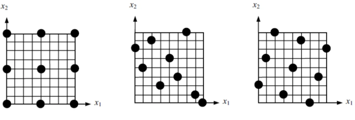
Latin hypercube sampling (LHS) designs start with the principle that if we have ny data points, then we should strive to have each variable have ny levels. This can be done by dividing the range of each variable into ny equal intervals and requiring that the variable has a level in each. Alternately, we can divide the range into ny-1 intervals and require that the variable has a value at the ny boundaries. This can still leave out large holes in the design space. So normally, LHS design is accompanied by a procedure that will optimize it to avoid large holes. Figure 4.4.4 compares three designs with 9 points.
Figure 4.4.1 Designs with 9 poinnts. The leftmost design is full factorial design with three levels. The middle one is a random LHS design, and the rightmost one is an LHS design optimized for maximum minimum distance between points.
The full factorial design has only three levels for each variable, the random LHS design has substantial empty regions on the top right and bottom left areas while the optimized LHS design has more uniform coverage.
It is not clear that for this particular case the LHS design is better than the full factorial design, because with a small rotation of the coordinate axes the full-factorial design would look better. Consequently, this is still a matter of controversy. However, optimal LHS designs allow us to specify any number of points, instead of being limited to special numbers associated with full-factorial or most of the other designs discussed earlier.
Matlab’s lhsdesign function produces LHS design with choice of two optimization strategies. One maximizes the minimum distance and the other minimizes a measure of the correlation between the variables.
Example 4.4.1:
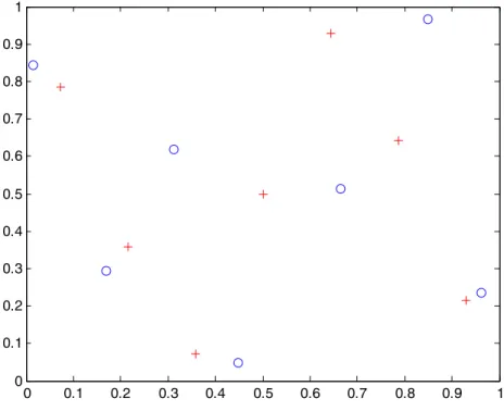
Generate two 7-point LHS designs in two dimensions using the two criteria and compare. >> x=lhsdesign(7,2,'criterion','correlation','iterations',1000) x1=x(:,1); >> x2=x(:,2); >> plot(x1,x2,'r+') >> x=lhsdesign(7,2,'criterion','maximin','iterations',1000); >> hold on >> x2b=x(:,2); >> x1b=x(:,1); >> plot(x1b,x2b,'o')
0 0.1 0.2 0.3 0.4 0.5 0.6 0.7 0.8 0.9 1 0 0.1 0.2 0.3 0.4 0.5 0.6 0.7 0.8 0.9 1
Figure 4.4.21: LHS designs. Plus symbols denote minimized correlation design and circles denote maximum minimum distance design.
It can be seen from the figure that there is not a great deal of difference between the designs. The minimum distance between the plus symbols (minimized correlation) is obviously somewhat smaller than between the circles (maximized minimum distance). The change in correlation between x1 and x2 is less obvious. It is -0.0714 for the pluses and -0.0777 for the circles.
4.5 Exercises
1. Find the maximum prediction variance in the unit cube for a linear polynomial, when the data is given in the four points (-1,-1,-1), (-1,-1,1), (-1,1,-1), (1,-1,-1).
2. Find the three points in the unit square that will minimize the maximum prediction variance in the unit square for a linear response surface.
3. For Example 4.3.1, find the maximum prediction variance for the minimum bias designs and compare it to that of the full factorial design.
4(*). Construct a minimum-bias central composite design. You may need to replace the central point with 4 points near the origin.