Learning to Predict Clinical Outcomes from Soft Tissue Sarcoma MRI

(1)

University of South Florida

Scholar Commons

Graduate Theses and Dissertations Graduate School

November 2017

Learning to Predict Clinical Outcomes from Soft

Tissue Sarcoma MRI

Hamidreza Farhidzadeh

University of South Florida, [email protected]

Follow this and additional works at:https://scholarcommons.usf.edu/etd Part of theComputer Engineering Commons

This Dissertation is brought to you for free and open access by the Graduate School at Scholar Commons. It has been accepted for inclusion in Graduate Theses and Dissertations by an authorized administrator of Scholar Commons. For more information, please contact

[email protected].

Scholar Commons Citation

Farhidzadeh, Hamidreza, "Learning to Predict Clinical Outcomes from Soft Tissue Sarcoma MRI" (2017).Graduate Theses and Dissertations.

(2)

Learning to Predict Clinical Outcomes from Soft Tissue Sarcoma MRI

by

Hamidreza Farhidzadeh

A dissertation submitted in partial fulfillment of the requirements for the degree of

Doctor of Philosophy

Department of Computer Science and Engineering College of Engineering

University of South Florida

Co-Major Professor: Dmitry Goldgof, Ph.D. Co-Major Professor: Lawrence Hall, Ph.D.

Rangachar Kasturi, Ph.D. Richard Gitlin, Sc.D.

Jacob Scott, M.D.

Date of Approval: November 6, 2017

Keywords: Image Processing, Tumor Heterogeneity, Radiomics, Deep Learning, Ensemble Bag of Visual Words

(3)

DEDICATION

I would like to dedicate this study and dissertation to my lovely family. My father and my

mother who support me in all aspects, continuously and steadily. Also, I want to dedicate

my dissertation to my lifelong friend, my brother, who without him, I couldn’t stand in this

(4)

ACKNOWLEDGMENTS

I would like to appreciate Dr. Dmirty Goldgof and Dr. Lawrance Hall because of their

constant support over last five years. I am thrilled to be guided by knowledgeable and

exceptional supervisors. With fruitful and insightful discussions, they directed me to boost

my study during my PhD. program.

I would like to address my sincere to our supporting group in Moffitt Cancer Center,

Dr. Meera Raghavan, Dr. Robert Gatenby and Dr. Robert Gillies. The foundation of

this research is established on the Soft Tissue Sarcomas data which are collected with this

team. Special thanks to Meera who devoted a lot of time to explain and clarify the basics of

biological background of this project while I was pretty new in this field. Likewise, I would

like to thanks Dr. Gateby and Dr. Gillies for suggestions and directions every time needed.

Furthermore, I want to express my appreciation to Dr. Scott and Dr. Joo Kim for their

support in sarcoma project as well as study on nasopharyngeal carcinoma tumors.

Finally, I want to thank my committee members for their valuable suggestions when

(5)

CHAPTER 3 METHODOLOGY 25

3.1 Proposed Methods Overview 25

3.2 Radiomics Framework 25

3.2.1 Region of Interest Delineation 26

3.2.1.1 Habitat Identification 27

3.2.2 Feature Extraction 28

3.2.2.1 Intensity Histogram Analysis 30 3.2.2.2 Quantitative Feature Analysis 32

(6)

3.2.4 Classification 40 3.3 An Ensemble of Bags of Visual Words 41

3.4 Summary 45

CHAPTER 4 RESULTS AND DISCUSSION 47

4.1 Summary of Datasets 47

4.2 Radiomics Analysis Results 49

4.2.1 Histogram Analysis 49

4.2.2 Summary of Histogram Analysis 55 4.2.3 Quantitative Feature Analysis Results 60 4.3 Ensemble of Bags of Visual Words Analysis Results 64

4.4 Methods Comparisons 66 CHAPTER 5 CONCLUSIONS 69 5.1 Summary 70 5.2 Future Work 71 REFERENCES 72 APPENDICES 85

Appendix A Reuse Permission 86

(7)

LIST OF TABLES

Table 2.1 Occurrence percentage of STS in different parts of the body 8

Table 3.1 Numbering the region of interest (ROI) 32

Table 3.2 GLRL and GLSZM features 38

Table 3.3 VGG-F deep architecture 44

Table 3.4 VGG-M deep architecture 44

Table 3.5 VGG-S deep architecture 44

Table 4.1 Summary of MCC and TCIA dataset 48

Table 4.2 Meta-classifiers description 50

Table 4.3 Best average result on 1D intensity histogram for metastasis development classification on MRI sequences in MCC dataset 50

Table 4.4 Best average result on 1D intensity histogram for necrosis rate classifica-tion on MRI sequences in MCC dataset 51

Table 4.5 Best average result on 1D intensity histogram for metastasis development classification on MRI sequences in TCIA dataset 52

Table 4.6 Numbering the region of interest (ROI) in MCC dataset 53

Table 4.7 Numbering the region of interest (ROI) in TCIA dataset 53

Table 4.8 The classification performance for prediction of metastasis for different spatial mapping habitats in pairs of sequences, TCIA dataset,

pretreat-ment images 55

Table 4.9 Evaluation of quantitative features for metastasis prediction on the MCC

data set 60

Table 4.10 Evaluation of quantitative features for necrosis prediction on the MCC

(8)

Table 4.11 Quantitative features evaluation for metastasis prediction on the TCIA

data set 62

Table 4.12 Evaluation of quantitative features from T1 pre-contrast within habi-tats for metastasis prediction for different spatial mapping habihabi-tats using pairs of sequences, TCIA dataset, pre-treatment images 62

Table 4.13 Evaluation of quantitative features from T2 for metastasis prediction for different spatial mapping habitats using pairs of sequences, TCIA

dataset, pre-treatment images 63

Table 4.14 BoVW evaluation on T1 pre-contrast for the metastasis development

task 65

Table 4.15 BoVW evaluation on T2 non-contrast for the metastasis development

task 65

Table 4.16 Evaluation of ensemble model on metastasis prediction on the MCC data

set 66

Table 4.17 Evaluation of ensemble model on metastasis prediction on the TCIA data

set 66

Table 4.18 BoVW evaluation on T1 pre-contrast for the metastasis development task, trained on MCC and tested on TCIA 67

Table 4.19 BoVW evaluation on T2 non-contrast for the metastasis development task, trained on MCC and tested on TCIA 67

Table 4.20 BoVW evaluation on T1 non-contrast for the metastasis development task, cross-validation on combined MCC and TCIA dataset 67

Table 4.21 BoVW evaluation on T2 non-contrast for the metastasis development task, cross-validation on combined MCC and TCIA dataset 67

(9)

LIST OF FIGURES

Figure 1.1 The dissertation scheme 4

Figure 2.1 Three MRI sequences 9

Figure 2.2 Transfer learning vs. traditional machine learning 14

Figure 2.3 Feature vector from bag of visual words model 17

Figure 2.4 BoVW framework in CBIR systems 18

Figure 3.1 Radiomics workflow on STS 26

Figure 3.2 ROI delineation and mask 27

Figure 3.3 Habitat on single MRI sequence 29

Figure 3.4 Overlapped habitats on multi-sequences MRI 30

Figure 3.5 Intensity histograms for ROIs 31

Figure 3.6 Difference intensity histograms 33

Figure 3.7 Corresponding original image (a), GLCM (b), GLRL (c) and GLSZM

(d) 36

Figure 3.8 Local binary patterns 37

Figure 3.9 Ensemble of bag of visual words 45

Figure 4.1 The classification performance for prediction of metastasis for different spatial mapping habitats sequence pairs for the MCC dataset,

Figure 4.2 The classification performance for prediction of necrosis rate for different spatial mapping habitats sequence pairs for the MCC dataset,

Figure 4.3 The classification performance for prediction of metastasis for difference of signal intensity with habitats, for pre-treatment and post-treatment images using sequence pairs for the MCC dataset 58

(10)

Figure 4.4 The classification performance for prediction of necrosis rate for dif-ference of signal intensity with habitats, for pre-treatment and post-treatment images using sequence pairs for the MCC dataset 59

(11)

ABSTRACT

Soft Tissue Sarcomas (STS) are among the most dangerous diseases, with a 50%

mor-tality rate in the USA in 2016. Heterogeneous responses to the treatments of the same

sub-type of STS as well as intra-tumor heterogeneity make the study of biopsies imprecise.

Radiologists make efforts to find non-invasive approaches to gather useful and important

information regarding characteristics and behaviors of STS tumors, such as aggressiveness

and recurrence. Quantitative image analysis is an approach to integrate information

ex-tracted using data science, such as data mining and machine learning with biological and

clinical data to assist radiologists in making the best recommendation on clinical trials and

the course of treatment.

The new methods in “Radiomics” extract meaningful features from medical imaging

data for diagnostic and prognostic goals. Furthermore, features extracted from

Convolu-tional Neural Networks (CNNs) are demonstrating very powerful and robust performance

in computer aided decision systems (CADs). Also, a well-known computer vision approach,

Bag of Visual Words, has recently been applied on imaging data for machine learning

pur-poses such as classification of different types of tumors based on their specific behavior and

phenotype. These approaches are not fully and widely investigated in STS.

This dissertation provides novel versions of image analysis based on Radiomics and Bag

of Visual Words integrated with deep features to quantify the heterogeneity of entire STS

as well as sub-regions, which have predictive and prognostic imaging features, from single

and multi-sequence Magnetic Resonance Imaging (MRI). STS are types of cancer which are

(12)

lung, brain and breast cancers. This dissertation does a comprehensive analysis on available

data in 2D and multi-slice to predict the behavior of the STS with regard to clinical outcomes

such as recurrence or metastasis and amount of tumor necrosis.

The experimental results using Radiomics as well as a new ensemble of Bags of

Vi-sual Words framework are promising with 91.66% classification accuracy and 0.91 AUC for

metastasis, using ensemble of Bags of Visual Words framework integrated with deep features,

and 82.44% classification accuracy with 0.63 AUC for necrosis progression, using Radiomics

(13)

CHAPTER 1 INTRODUCTION

1_{In the health care field, diagnostic and prognostic medical imaging plays a pivotal role}

in planning and deciding on care or therapy regimes. Traditionally, expert radiologists,

pathologists, and clinicians intensively carry out qualitative and quantitative assessments.

They aim to assess the right therapy along with the right dosages, at the right time to get

the best results from clinical trials, in a process known as “precision medicine” [1]. However,

this procedure is time consuming and costly because it relies on the experts’ knowledge.

“Big data analysis” [2] aims to discover unseen correlations and useful information in

large databases. Dealing with a large amount of data in different categories (e.g clinical data,

Magnetic Resonance Imaging (MRI) or Computed Tomography (CT)) is demanding new and

novel data mining approaches to do underlying analysis for prediction (e.g classification or

clustering). Computational and mathematical based methods in computer science, which

include data mining and machine learning, are indispensable tools to use for quantitative

analyses and evaluations. Integration of machine learning and data mining with clinical

knowledge is the basis of the Computer Aided-Diagnostic (CAD) systems. CAD systems

can assist clinicians to optimize a therapy plan to get the best outcome and yield less risk

in earlier stages of treatment.

Additionally, it would be desirable to consider a non-destructive approach when doing

tumor diagnosis. Instead of resection for biopsies, which is invasive and potentially causes

1_{Part of this chapter is partially from recently published paper: ”Hamidreza Farhidzadeh, Dmitry B}

Goldgof, Lawrence O Hall, Jacob G Scott, Robert A Gatenby, Robert J Gillies, and Meera Raghavan. A quantitative histogram-based approach to predict treatment outcome for soft tissue sarcomas using pre-and posttreatment mris. In 2016 IEEE International Conference on Systems, Man, and Cybernetics. IEEE, 2016”. The reuse permission is in Appendix A.

(14)

bleeding, infection and other side effects, MRI sequences offer a non-invasive option for tumor

diagnosis. MRIs, in different sequences, can be used to extract many mineable imaging

features and characteristics, which are associated with cellularity and blood flow in-vivo [3].

As a result, intra-tumoral functional features related to tumor can be assessed. Intra-tumor

diversity and variability contain information which should be explored. Thus, MRIs play

the key role in the initial step of data acquisition.

After data acquisition, we will have obtained data sets of medical images for quantitative

analysis. To perform quantitative analysis, learned models are capable of providing valuable

information to enhance the diagnosis. The learned models extract mineable information

from MRI scans, generate the predictive framework, and given a test image, prognosticate

the clinical outcome, particularly tumor recurrence or metastasis and necrosis. However, the

primary challenges raised include the way in which information such as imaging bio-markers

can be captured in a meaningful way. Further, it must be decided how machine learning

methods could be helpful with MR images and relevant clinical information as an input

towards an image-guided therapy assistant.

1.1 Motivation and Challenges

Tumors that occur in soft tissues such as muscles, fat and nerves are called Soft Tissue

Tumors (STT). Generally speaking, there are two categorizations for these tumors:

malig-nant and benign. In maligmalig-nant tumors, cancerous cells spread out through other sections

of the body via blood flow. The term “Sarcoma” identifies a malignant tumor. Soft Tissue

Sarcomas (STS) are an aggressive group of lesions within soft tissue such as fat, muscle,

and nerves structure. According to the American Cancer Society2_{, there are 50 subtypes}

of sarcomas. They also reported that 12,310 patients suffered from STS in 2016 and about

50% of them die because of STS. It is desirable for radiologists to optimize (personalize) the

2

(15)

treatment regimen at the initial stage of treatment. Ideally, quantification of tumor

charac-teristics would be helpful to select the most effective therapy approach such as radiation or

chemotherapy for each patient. However, the main problem in this step is the heterogeneity

of STS.

Genetic and phenotypic variability exist between tumors and within the same tumor,

which are known as inter-tumor and intra-tumor heterogeneity, respectively [4]. Generally,

tumor cancers exhibit intra-tumor heterogeneity in various phenotypic features, such as in

gene expression, metabolism and metastatic cancer cells [5, 6, 7, 8]. The present view on

tumor heterogeneity is rooted in Darwinian evolution and ecology [9]. Intra-tumoral diversity

can emerge at the epigenetic level [10] and at multiple genetic levels [11, 12]. Ultimately,

tumor heterogeneity causes substantial negative effects on tumor prognosis, weakens the

understanding of intra-tumor interactions and confounds future drug-development methods

[4].

STSs are heterogeneous groups of tumors. Due to intra-tumoral heterogeneity; for

pa-tients with the same tumor stages, different responses to the treatment are observed.

Tempo-ral and spatial heterogeneity of STS make its quantification challenging. As previously

men-tioned, with a 50% mortality rate, it is essential to look for the right and precise treatments

to address aggressiveness of a tumor at an earlier stage of its development. Identifying the

right treatment can reduce the morbidity caused by chemotherapy and radiation [13, 14, 15].

To boost the optimal (personalized) treatment, it is important to distinguish the type

of tumor based on imaging bio-markers. This work looks deeply into these challenges and

presents methodologies with regard to quantitative image analysis and learning models. The

(16)

1.2 Contributions

The main target of this study is to integrate the STS tumor radiology using medical

oncology with learned models associated generated by data science which make use of image

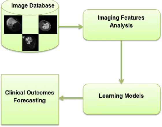
processing and machine learning. Generally speaking, the outline of the study is summarized

and illustrated in Figure 1.1.

Figure 1.1. The dissertation scheme

The general scheme of this work is to quantify the intra-tumor heterogeneity in a

non-invasive fashion. This work considers imaging biomarkers for the entire tumor as a Region of

Interest (ROI), as well as the tumor’s “habitats” [16]. In [16], authors proposed that regional

variations in imaging variables, such as contrast intensity which is controlled by blood flow,

(17)

tumor as a union of tumor habitats. The imaging parameters associated with each habitat

are captured and quantified to examine it’s contribution in clinical outcome forecasting.

1.2.1 Intra-tumor Heterogeneity Quantification with Imaging Features

We investigated the entire tumor as well as tumor habitats to extract and represent

imaging features to quantify STS heterogeneity. This is the first study in quantitative image

analysis on STS to explore the presence of tumor habitats defined by contrast intensities

variation in a single sequence and spatial mapping analysis on multiple MRI sequences.

After habitat identification, we analyzed different types of Radiomics features [17] such as

contrast enhancement intensity, texture and morphological features as well as deep features

[18], which are extracted from pre-trained deep neural network architectures [19, 20]. To

extract the deep features, we follow the transfer learning [21, 22] idea. The novelty of this

work, in addition to the habitat identification of STS tumors, is to capture local binary

patterns as a texture feature and make use of deep features.

1.2.2 Ensemble Bags of Visual Words Framework

Bag of words (BoW) [23] is a well-known approach to classify documents based on

fre-quency of words which is employed to train classifiers. Bags of Visual Words (BoVW) is a

derived version of BoW which is designed for computer vision [24]. In this study, for the

first time we are using the novel BoVW model for STS classification.

The integration of different feature extractors, here pre-trained CNNs, and different

clas-sifiers is a key part of developing a BoVW model which is called Bags of Visual Words. This

framework uses deep features, derived from same-sized patches extracted from the whole

tu-mor, to explore the intra-tumor variations. Histograms of visual words are treated as input

for training the classifiers and ultimately the aggregation of predicted outputs classifies the

(18)

To summarize, the first contribution is based on the idea that imaging bio-markers derived

from each tumor habitat [16] will have different capabilities for identifying clinical outcomes.

For the first time, we examined the STS as a coalition of distinctive habitats and compared

the prediction ability of derived imaging features from different parts of the tumor regarding

metastasis development and necrosis rate. This contribution is central for image processing

and machine learning techniques.

The second contribution is based on computer vision technique, Bag of Visual Words.

Here, for the first time, we used a transfer learning approach to capture deep features out

of the entire tumor to create a feature vector. Also, we built a new ensemble framework to

classify the STS regarding prediction for metastasis development.

1.2.3 Model Applications

Surgical resection can cure primary tumors; however metastatic tumors are widely

in-curable due to the diffusion throughout the body of tumor cells. According to [25, 26] more

than 90% of patients who suffer from cancer die due to metastasis, not the primary tumor.

As a result, effective and efficient cancer medication and treatment is highly correlated with

the ability to prevent the metastasis process. By using quantitative image analysis, we assay

the regional and micro-environmental variations to characterize the likelihood of metastatic

tumor for further consideration.

Another factor used to assay the STS is the necrosis rate of tumor cells in biopsies which

is the gold-standard evaluation method [27]. Based on the tumor necrosis percentage in

re-sected specimens, there are histological classifications that separate good and bad treatment

responders [27]. The discriminator threshold to separate good and bad treatment responders

is set as 90% of tumor exhibiting necrosis. Good treatment responders show more than a

(19)

tumor necrosis rate. This rate is computed as the fraction of necrotic tumor size over total

tumor size [27].

The proposed frameworks are applied on described data sets to evaluate the performance

in classifying metastatic and non-metastatic STS, as well as necrosis.

1.3 Dissertation Overview

The dissertation contains five chapters. The second chapter mainly discusses data science

(e.g. image processing and computer vision as well as data mining and machine learning)

for bio-medical applications in oncology. Chapter 3 presents a detailed explanation of the

proposed methodologies associated with Radiomics and BoVW analysis on identified

habi-tats. Chapter 4 shows the comprehensive and complete experimental results of the proposed

(20)

CHAPTER 2 BACKGROUND

This chapter discusses the general concepts regarding Soft Tissue Sarcomas and its

tax-onomy, the common MRI sequences used on STS, data science in biomedical engineering,

feature reduction and selection, machine learning strategies, and machine learning classifier

evaluation metrics.

2.1 What are Soft Tissue Sarcomas

The out of control growth of cells in the body results in cancers. Generally, a sarcoma

tumor is a type of tumor which arises from a certain part of the body, either bone or soft

tissues. Soft Tissue Sarcomas occur from soft tissue such as nerves, fibrous structures and

muscles. They can reside in the body’s structures for a long time before being discovered1_.

Table 2.1. Occurrence percentage of STS in different parts of the body Body Part Occurrence Percentage

Head & Neck 6%

Thoracic 9% Visceral 13% Upper Exremity 13% Retroperitoneal Intra-abdominal 27% Lower Exremity 32%

These are rare tumors that arise in different parts of the body. Table 2.1 is from the

Chicago Cancer Surgery Center2 which illustrates the percentage of STS occurrence in

dif-1

http://www.cancer.org/cancer/sarcoma-adultsofttissuecancer/detailedguide/sarcoma-adult-soft-tissue-cancer-soft-tissue-sarcoma

(21)

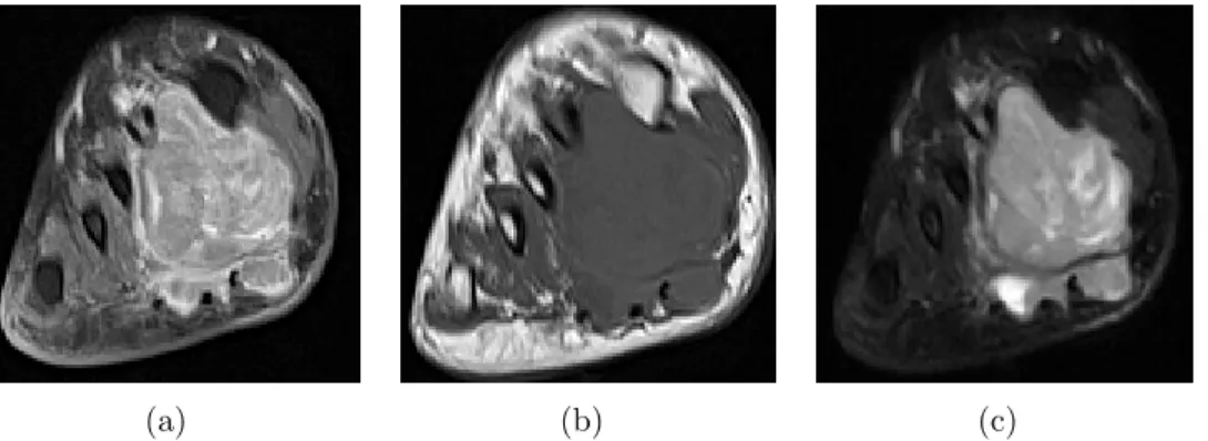
(a) (b) (c)

Figure 2.1. Three MRI sequences. (a) T1 post-contrast (b) T1 pre-contrast (c) T2 non-contrast of Soft tissue Sarcomas from private dataset

ferent regions of the human body. According to the Table 2.1, it is understood that the

majority of STS (almost 1/3) develop from lower extremities and only 6% of them are in the

head and neck.

2.2 Soft Tissue Sarcomas in MRI Sequences

MRI can detect blood flow and malformations in vessels as well as demyelinating disease

and simplify visualization of the posterior fossa [28, 29, 30, 31]. Radiographic parameters

can also be revealed in cross-sectional MRI radiology images. It also enables visualization of

the tumor environment from different angles which are the axial, coronal and sagittal planes.

Thus, it is worthwhile to utilize these imaging data to assess the tumor heterogeneity.

There are multiple MRI protocols that provide detail of tumor vascular anatomy: T1

pre/post-contrast and T2 non-contrast. The contrast enhancement is predominately

ob-served in T1 sequences after contrast agent (gadolinium chelates) injection. Enhancement

discriminates between the colony of the cancerous cell, which are ceaselessly absorbing blood

and non-active regions. The active region, due to high blood flow, has high (enhanced) signal

intensity. As a complementary sequence, T2 identifies the watery cells within the tumor and

demonstrates cellularity. The bright spots contain water, while fat and air appear dark [32].

(22)

2.3 Feature Extraction and Representation

A key initial step in building learning models from imaging data is feature extraction. The

feature extraction objective is to quantitatively obtain useful information from the biology

and environment of the tumor as represented in MRIs that could result in case-specific

patterns for making medical decisions. Mathematically, in this stage of imaging analysis,

features, which are correlated to tumor biology and discriminative enough, are desirable.

This section reviews popular image features for biomedical applications such as Radiomics

features. Also, it covers the state-of-art feature representation [33], Bag of Visual Words as

well as a new feature learning approach, Deep Learning [34].

2.3.1 Radiomics Features

As previously mentioned, Radiomics analyses [35] include a group of methods to

ex-tract features from radiographic images, mine them, and ultimately utilize them for clinical

decision making purposes. Radiomics features are associated with contrast enhancement

voxel/pixel intensity, texture and morphological (e.g shape and color) features.

• Signal Intensity Features: These features are from first-order statistics [36] and are derived from a histogram of intensities. The first order is related to the distribution of

gray-level frequency within the ROI. The statistics of this level are based on a histogram

of intensity, consisting of mean, maximum, minimum intensity and standard deviation

of the gray-level histogram, irregularity of gray level distribution (entropy), uniformity

of distribution (uniformity), flatness of the histogram (kurtosis) and asymmetry of the

histogram (skewness).

• Texture Features: Texture features [37] are second-order statistics. The second level features are related to co-occurrence measurements by using a gray-level dependence

(23)

intensities. Well-known second order features include the Gray-level Co-occurrence

Matrix (GLCM) [37], Gray-level Run-Length Matrix (GLRLM) [38, 39, 40, 41] and

Gray-level Size Zone Matrix (GLSZM) [38, 41, 39, 40].

Local Binary Patterns (LBP) [42], Scale Invariant Feature Transform (SIFT) [43] and

Histogram of Oriented Gradients (HOG) [44] also are popular robust descriptors which

are abstracted from the computer vision domain.

The third order of features is hierarchically built on the first and second level of feature

layers. They depend on gray-tone-difference matrices to test the spatial interaction of a

pixel value and its neighborhoods (e.g. NGTDM: Neighborhood Gray-Tone Difference

Matrix [45]).

• Morphological Features: These features are obtained from geometric attributes of the tumor. Generally, they include: size, diameter, color, solidity and eccentricity.

Recently, radiomics analyses have been used for different biomedical applications,

es-pecially in tumor cancer classification. Chicklore et al. [46] reviewed radiomics features

analysis in 18_{FDG PET/CT to measure the spatial variation within the tumor and its}

prog-nostic information in determining response to the treatment in an early stage rather than

using standardized uptake value (SUV), because the prognosis ability of SUVs from a

base-line scan is limited. In [47, 48, 49, 50], Aerts group from Harvard Medical School worked on

Lung and Head and Neck cancer, using clustering to deal with high dimensional radiomics

feature space (440 radiomics features) and discovered common radiomics patterns. They

have used radiomics features for classification of head and neck and lung cancers based on

survival time (they dichotomized the survival data using a cutoff time of 2 years for lung

and 3 years for head and neck cancer.). In [51] a novel quantitative radiomics feature

analy-sis from multiparametric MRI (mpMRI) was proposed to perform prostate cancer detection.

(24)

tumor candidate regions. On breast cancer, [52, 53, 54, 55, 56, 57] presented studies

regard-ing radiomics feature analyses on identified radiological habitats to predict Axillary lymph

node (ALN) metastases and Estrogen receptor (ER) status. Likewise, [58, 59, 60, 61, 62, 63]

conducted radiomics analysis to classify the Glioblastoma (GBM) brain tumor regarding

survival time based on identified radiological habitats. In [64], Vallieres et al. quantified

the tumor heterogeneity to stratify the metastatic STS using radiomics features. In [65],

we used Radiomics to predict progression free survival in Head and Neck (Nasopharyngeal

Carcinoma) cancer. Also, in line with the dissertation, multiple contributions were published

[3, 66, 67, 68, 69] which will be explained in the next chapter.

2.3.2 Deep Features

The primary idea of deep learning algorithms is to stack up the non-linear

transforma-tion layers. These consist of convolutransforma-tion, pooling (i.e max or average) and rectifying [70]

layers. The main goal is to obtain complex representations of input data from a hierarchical

structure, where layers at the lower levels (closer to the input layer) capture more generic

complex representations of data, while higher level layers create case-specific representations

[71]. By adding more layers to the architecture of the deep learning model, more complex

non-linear transformations are built to extract important attributes of input data [72, 73].

The resultant attributes can be extracted and utilized as input features to train machine

learning classifiers.

Two main applications of deep learning algorithms are segmentation [74] and classification

[75] tasks. To perform the segmentation task, auto-encoders are widely used, especially in

brain segmentation [76, 77, 78, 79]. U-net [80] is a new model which won the ISBI cell tracking

challenge 2015 for microscopy images. The auto-encoders or auto-associators [81] manipulate

(25)

target is to visualize the reconstructed input. To obtain this goal, in their architecture, the

deconvolution layers [82] are succeeded by convolutional layers.

To do classification tasks on images, Convolutional Neural Networks (CNNs) are very

popular. The pioneering CNN, called LeNet, was proposed by LeCun [83] to classify

hand-written digits. In biomedical applications, recently, researchers are making efforts to design

a deep learning model for their classification purposes. For lung nodules [84, 85, 86, 87], for

breast cancer [88, 89, 90] and for brain tumor classification [91, 92] deep learning algorithms

have been applied.

2.3.3 Transfer Learning from Deep Learning Models

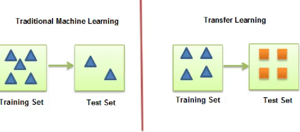
Generally speaking, transfer learning (also known as inductive transfer) [21, 93] means

using the obtained knowledge from a particular problem in a specific domain, and applying

it to another problem from a different domain. To be specific, in the machine learning area,

in contrast to traditional machine leaning approaches in which training and testing data

are from same domain (e.g brain images), in transfer learning training and testing data can

be from different domains (e.g training data contains natural images while testing data has

biomedical images). Figure 2.2 illustrates this comparison.

Using CNN as a feature extractor or fine-tuning the CNN are two approaches to transfer

learning using deep learning algorithms [94, 95]. The CNN pre-trained on ImageNet3 [96]

without the last classifier layer (fully-connected layer) can be treated as a feature extractor

for input images from any category.

The second approach is to fine-tune the CNN weights of a pre-trained network by

con-tinuing the backpropagation training process, instead of training the network from scratch.

Recently, Tajbakhsh [97] showed that in some medical imaging applications fine-tuning

(26)

Figure 2.2. Transfer learning vs. traditional machine learning

performed the full-training of the CNNs and the fine-tuned CNNs are more robust when the

size of the training set is small.

2.4 Bag of Visual Words

Bag of Words templates were invented for use in information retrieval to simplify

docu-ment representation. In a BoW model, docudocu-ments are transformed into histograms of words.

From a machine learning point of view, these histograms are feature sets to train the

classi-fier to do the document classification task. Each element of the feature vector is the count

of the number of times a word occurs.

The derived version of the BoW model for the computer vision field is the Bag of Visual

Words (BoVW) model in which the features are “visual words” instead of actual words

in a language. The visual words are the feature representations of image attributes from

primitive (low) level features to abstract (high) level features. Primitive features are image

attributes such as color, shape and texture (e.g. features obtained from flowers) while high

level features are semantic attributes require some reasoning to deduce meaning (e.g features

(27)

The BoVW models are the basis of the content-based image retrieval (CBIR) systems [99]

which match the extracted primitive image features, such as texture, from training images

with the query (test) image. The highest matching score between training images and query

image results in the assignment of the class of the query image.

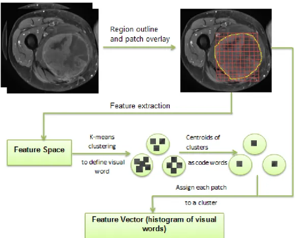
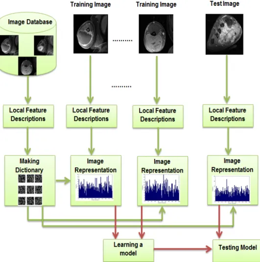
CBIR in medical imaging applications [100, 101] contains the following steps (Figures 2.3

and 2.4):

1. Local Feature Description: First, from training set images, some underlying

compo-nents associated with the whole image should be identified. For example, using SIFT,

there are some keypoints within the image used to describe the image. However, in

medical images, as all points (pixels) within the ROI are interest points, it would be

computationally intensive to explore all the points. Instead, same size patches,

con-sisting of multiple pixels (e.g. 16×16 pixels), are extracted from the ROI for local attribute description.

To explain this step, let’s follow an example. Suppose we haveN images in the training

set and extract a different number of patches out of the images (obviously, as the size

of the ROIs are different across images, the number of extracted patches are different,

as well. Any patch, which has more than half of its area covered by tumor tissue, is of

interest and will be processed). Suppose in total, there are M patches from whole the

training set (For image i, mi patches are extracted, s.t.

P

Nmi = M). Next, a fixed

number of features F are captured from each patch (the feature space is of dimension

F).

2. Visual Dictionary Generation: K-means clustering [102] on the feature space

deter-mines the size of the dictionary, or simply the number of words in the dictionary which

are centroids of the clusters. The size of the dictionary (K) is a gray area as some

(28)

while others [101] indicate the dictionary size matters in medical image classification

tasks.

3. Image Representation: In this step, the images in the training set are transformed into

a histogram of visual words.

Based on our example, the algorithms starts to analyze each image in the training set.

It uses a simple nearest neighbor algorithm (with Euclidean distance) between each

patch of the image and K centroids of clusters to see which of centroids (visual words

here) is closest to the patch (using features extracted from step 1) as shown in Figure

2.3. The word histogram of each image is generated when all the patches are each

assigned to one of the words in the dictionary. The histogram consists of a vector of

size K where each entry is the number of patches assigned to the ith (1 ≤ i ≤ K) word (a number between 0 and number of patches).

4. Training a Classifier: The word histograms captured from the previous step are the

input feature vectors for learning a model such as an SVM or K-nearest Neighbor [102].

5. Test: After generating the image representation (visual bag of words representation)

of the incoming image, we can use our trained model to classify the test image.

In [101], authors employed abag of feature framework to classify histopathological images

from 18 categories. In [104] authors proposed a mutual information based word selection

method to improve the classification rate of three separate datasets of chest x-rays, liver

lesion CT images and mammography micro-calcifications images. In [105], the authors used

a patch-based visual words framework on the ImageCLEF4 _{dataset as well as a chest x-ray}

with 98 frontal chest images (separate dataset). By proposing the bag of semantic words

model, [106] fills the gap between the primitive image features and medical concepts. It

concluded that the extracted semantic information from the ADNI dataset [107] can enhance

(29)

Figure 2.3. Feature vector from bag of visual words model

the classification rate. For lung nodule classification [108] proposed a novel adaptive

multi-level framework in which instead of same size patches, clustered regions using superpixel

formation on signal intensities are used as the image components.

2.5 Feature Selection

In the feature extraction step, the main goal is to get a concise and unique representation

of the object. The feature selection process obtains a subset of features which one hopes does

not have irrelevant and redundant information and also preserves the original discriminative

information [109]. Feature selection methods try to reduce model computation time (with

fewer features) and boost prognostication. To select the subset, which reduces dimensionality,

(30)

Figure 2.4. BoVW framework in CBIR systems

The feature selection methods belong to two main categories: filter and wrapper

meth-ods [110]. In the filter method, the features are ordered independent of the classifier, and

only high ranked features are utilized as the pattern from which to do classification. In the

wrapper method, the learning algorithm ranks the feature subset with regard to the highest

classification accuracy for a specific classifier.

• Filter Method: Filter methods use feature ranking approaches to select features. Us-ing orderUs-ing methods provides simplicity and has had reasonable success for different

(31)

data before classification to remove the less relevant features. A feature which can

provide discriminant information about different classes is favorable. This is so-called

relevancy which quantifies the feature discrimination ability for different classes. To

measure the relevancy of the feature, there are multiple efforts [111, 112]. One

crite-rion for irrelevancy is that a feature is weakly dependent on the target class [113]. The

feature is ignored when there is no correlation with or predictive ability for the class

label. The best feature subset is not unique because of the unknown underlying

distri-bution and a classifier may obtain the same accuracy by using different sets of features.

Some methods in this category are mutual information [114], Fisher score [115], and

RELIEF-F [116].

• Wrapper Method: In wrapper methods, the predictor performance using the selected feature subset is the objective function for evaluation. To find the optimal subset, at

each step (iteration) a feature set of size x(1, n) (n is the total number of features)

is tested to maximize prediction performance. As an example, branch and bound

methods [117] employ a tree structure to weight different feature subsets. However,

the drawback of this approach is exponential growth in the search space for the large

feature set.

Wrapper methods use sequential search and heuristic search algorithms. The sequential

search algorithms are iterative. The Sequential Feature Selection (SFS) algorithm [118]

initializes an empty feature set and adds one feature in each step to obtain maximum

classification performance. The feature which enables maximum classification accuracy

will remain in the feature subset. No more features are added to the subset when

accuracy does not improve. The Sequential Backward Selection (SBS) algorithm is like

SFS but in reverse, which means it starts with a full subset of features and removes a

feature at each iteration such that losing that feature yields minimum or no reduction

(32)

The heuristic search algorithms optimize the prediction performance by evaluating

different subsets. The Genetic Algorithm and Particle Swarm Optimization are in this

category [119].

The main drawback of wrapper methods is the high computational complexity to find

the best feature subset. For each subset, the classifier makes a new model in which the

classifier is trained on a feature subset and tested for performance. For large datasets,

most of the time is spent on training. Over fitting is also a weakness of these methods.

It occurs when the classifier is trained to tightly fit the training data and loses it’s

generalization ability for unseen data. Over fitting leads to a higher classification error

rate because it makes the classifier biased towards the training data. To ease this

problem a holdout validation set could be applied to enhance prediction accuracy.

Dimensionality reduction tries to project high dimensional data into a meaningful

repre-sentation in a lower dimension. As dimension reduction relieves the curse of dimensionality

and potentially some unfavorable properties of data, it is widely applicable. In medical

imag-ing data, dimensionality reduction has been applied for different applications [120, 121, 122].

There are two main classes of dimension reduction methods: linear and nonlinear methods.

The linear methods are simpler, but they cannot handle the complex nonlinear data.

Two well-known linear dimension reduction methods are Principal Component Analysis

(PCA) and Linear Discriminant Analysis (LDA) [123]. PCA [124] is an unsupervised linear

technique which performs dimension reduction by creating orthogonal vectors which explain

the data variance [125]. It computes the mean vector and co-variance matrix of variables as

well as eigenvalues and eigenvectors. It sorts eigenvectors according to decreasing eigenvalues

and uses theK largest eigenvectors. PCA has been used in various types of studies on several

cancers [126, 127]. PCA does not consider the difference between classes of data, but LDA

(33)

construct a low dimension subspace by minimizing intra-class and maximizing inter-class

variances.

2.6 Learning Strategies

Machine learning techniques have been broadly used for medical image analysis in

differ-ent applications such as tumor segmdiffer-entation [128] and cancer type prediction [66]. Based on

available data and the target task, a proper model can be designed. In regard to utilization

of the labels of training data, machine learning algorithms are supervised, unsupervised and

semi-supervised.

In supervised learning, the target is to learn the model from training data with known

class labels to forecast the label of the unknown input patterns from unseen data.

Unsuper-vised learning is used to find structure in data without having any labels. Semi-superUnsuper-vised

learning is a hybrid approach which takes a small portion of labeled training data. The

un-labeled data are used in the learning process as well, instead of being untouched [129, 130].

In case of STS, supervised learning has been used in some efforts [131, 132, 133, 134].

Supervised learning contains two steps: the training and testing step. The classifier will

use the training data with class labels in the training step. The classifier performance is

evaluated by a predicted label compared with ground truth in the testing step. To sum

up, the goal of supervised learning is to build a predictive model from training samples and

generalize to testing samples. For example, in [132], authors used gene expression profiling

to classify different subtypes of STS and in [134], authors used texture features to classify

benign and malignant STTs.

The unsupervised learning methods have also been used for medical imaging data

analy-sis [132, 135, 136]. In unsupervised learning, there exists a set of unlabeled observations with

no information about the class of each sample. It groups the unlabeled data based on mutual

(34)

target of study in [137] was to classify clear cell sarcoma (CCS) as either soft tissue sarcoma

or typical melanoma. CCS has common features with both soft tissue sarcoma and typical

melanoma. Authors used gene expression profiles as features and an unsupervised learning

technique and finally concluded that CCS is a distinct genomic subtype of typical melanoma.

In [6], authors clustered subtypes of STS by using gene profile expressions.

Semi-supervised learning is well-suited in tasks for which it is difficult to find the class

labels for certain samples. In other words, this hybrid approach is designed to overcome

the limitation of supervised learning which is incapable of training with data with missing

labels. In [138] semi-supervised methods on gene expression profiling have been used to

predict cancer recurrence. The authors integrated gene expression with Protein-Protein

Interaction (PPI) and recognized the informative gene pairs with the labeled instances, and

then built an instance based graph model using selected genes to make a semi-supervised

learning classifier.

2.7 Evaluation Metrics

The performance of the two-class classifier is usually represented in a confusion matrix.

The entries of a confusion matrix show whether the samples are correctly or incorrectly

classified. One of the methods to evaluate the learning algorithms performance is

cross-validation [139].

The cross-validation method divides samples into two partitions: one is used to learn or

train a model, and the other unseen part is used to validate the model. K-fold cross validation

and the special case of it, leave-one-out cross-validation, is used to evaluate classification

algorithms. For K-fold cross validation, the process iteratively proceeds K times. At each

round, the data is divided into K approximately equal sized subsets, K-1 of the subsets are

(35)

In the leave-one-out method, only one instance from the dataset is chosen as the testing

set; all remaining samples are considered as training samples. The performance of the

learning algorithms for a two class problem is determined by the True Positives (TP), True

Negatives (TN), False Positives (FP), and False Negatives (FN) that indicate samples which

are correctly classified, correctly rejected, incorrectly classified, and incorrectly rejected,

respectively. The accuracy of the learning algorithm is defined by:

Accuracy = _{T P}₊_{T N}T P+₊T N_{F P}₊_{F N}

There are other metrics to evaluate learning algorithm performance. Sensitivity or recall,

measures the rate of correctly classified instances (true positive rate). Specificity measures

the rate of correctly rejected instances (true negative rate). Precision measures positive

predictive value.

Sensitivity = _{T P}T P₊_{F N}, Specif icity= _{F P}T N₊_{T N},P recision= _{F P}T P₊_{T P}

The F-measure and G-measure also combine the precision and recall in terms of a compatible

mean:

F −measure= 2×P recision×Recall P recision+Recall, G=

√

P recision×Recall

Receiver Operating Characteristic (ROC) analysis and Area Under Curve (AUC) are also

popular to evaluate the performance of the algorithm [134].

2.8 Summary

To conduct quantitative medical image analysis, it is imperative to utilize data science

knowledge i.e image processing, computer vision, and data mining. After delineation of the

ROI within the medical image, the ROI attributes should be translated into mathematical

(36)

Radiomics features as well as deep features have gained popularity recently to describe

image characteristics. Not all extracted features have underlying discriminative capability,

and some good features can be correlated with others, which is not helpful. Thus, removing

these variables can be helpful in improving accuracy and training time when learning a

model. By training the supervised classifier with a predictive subset of features, the trained

(37)

CHAPTER 3 METHODOLOGY

3.1 Proposed Methods Overview

1_{This work presents novel and new quantitative images analysis frameworks to quantify}

the heterogeneity of Soft Tissue Sarcomas from the whole tumor as well as tumor habitats.

The frameworks begin with pre-processing and ROI detection and continue with feature

extraction and finally classification.

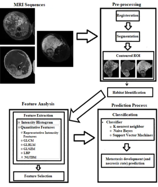
3.2 Radiomics Framework

This section proposes a Radiomics framework for quantitative image analysis on STS

MRI. Figure 3.1 shows the Radiomics workflow.

As pixel level values or gray-level signal intensity values are the most easily observable

image attributes, first we analyze the intensity histogram of ROIs as imaging features and

weigh its ability in outcome prediction.

Besides that, the framework captures representative first order statistics of the intensity

histogram as well as second and third order statistics, which are associated with the texture

parameters within the ROI. The captured features should be purified by removing redundant

and irrelevant features using feature selection techniques and finally, the best subset of

features are input variables into a machine learned classifier.

1_{Parts of this chapter were published in the SPIE Medical Imaging Proceedings and IEEE Systems, Man}

and Cybernetics (SMC) Proceedings [3, 66, 67, 68, 69]. The copyright permissions to reuse the contents are in Appendix A.

(38)

Figure 3.1. Radiomics workflow on STS

The ROIs are either the entire tumor or the tumor habitats. The next part explains a

method to identify the habitats.

3.2.1 Region of Interest Delineation

The input data for our framework are either 2D or multi-slice MRIs of STS tumor

im-ages. The images are in T1 pre/post contrast (which measures the vascular blood flow) and

(39)

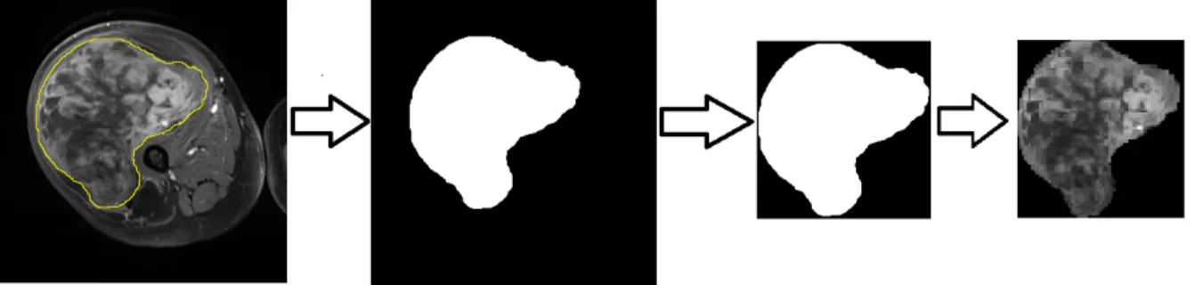
techniques such as in [140] and particularly for STS [141], an expert radiologist manually

contoured (yellow line in Figure 3.2) the ROI to have reliable ground truth. After manual

delineation, a binary mask is created where the tumor areas are represented in white and

healthy tissue and background is shown in black. The tightest box which includes the ROI

is the final mask. By mapping the mask to the MRI image the final outcome is obtained

(the final square with ROI in it). This process is shown in Figure 3.2. The captured mask

is applied to all modalities which are registered. In the framework which extracts attributes

from the entire tumor, the masked images are used as input for the system. To quantify the

intra-tumor regional based spatial variations, we followed by idea of “habitats” [16]. This is

the first work that measures the tumor variation in underlying sub-regions on STS tumors.

Figure 3.2. ROI delineation and mask

3.2.1.1 Habitat Identification

The concept of habitats considers the entire tumor as an integration of different

sub-regions which have various imaging attributes and functionalities. To define specific habitats,

we applied the Otsu segmentation method [142] to divide the tumor into two sets of signal

intensity groups. It iteratively looks for the grey level threshold in grey levels which is the

optimal cut-off point to separate the image into two classes by maximizing the between class

variance as well as minimizing within class variance.

(40)

σ

_b2

=

β

1

(

µ

1

−

µ

2

)

2

+

β

2

(

µ

1

−

µ

2

)

2

where σ2

w,σb2, β1,β2, µ1 and µ2 are, inter-class and intra-class variances, class probabilities

for divided pixels and average pixel value for different classes, respectively.

• Single Sequence Habitats: Simply, by applying the Otsu segmentation on different imaging sequences individually, different sub-regions are obtained as shown in Figure

3.3 as an example.

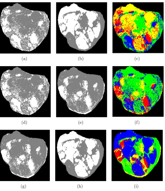
• Multi-Sequences Habitats: As mentioned before, different MRI sequences identify unique tumor attributes. Combined habitats already show promising results on brain

[61] to predict the survival time of Giloblastoma Multiforme (GBM) and breast

tu-mors [57] to predict Axillary lymph node (ALN) metastases and Estrogen receptor

(ER) status. Following the idea proposed in [61], we extracted combined habitats by

intersecting signal intensity classes of individual sequences. Figure 3.4 shows Otsu

segmentation on T1 post-contrast presented in (a and d), Otsu segmentation on T2

non-contrast presented in (b and h), Otsu segmentation on T1 pre-contrast presented

in (e and g), and (c, f and i) are the intersection results.

After defining the ROI, i.e. entire tumor, habitats within a single sequence or a combined

habitat using multi-sequence MRIs, the next phase is to obtain features.

3.2.2 Feature Extraction

This section describes the feature extraction in pixel gray level values, as well as higher

order of statistics. For intensity histogram analysis, we used the method proposed in GBM

prognostication [61] as it showed promising results. Then, instead of working on pixel level

features, first order statistics as well as second and third order statistics were evaluated in

(41)

Figure 3.3. Habitat on single MRI sequence. T1 post/pre contrast and T2 from up to down (while region is high signal group and gray region is low signal group)

(42)

(a) (b) (c)

(d) (e) (f)

(g) (h) (i)

Figure 3.4. Overlapped habitats on multi-sequences MRI

3.2.2.1 Intensity Histogram Analysis

As previously mentioned, different MRI protocols capture underlying imaging biomarkers

and identify diverse characteristics of the ROI. The T1 sequence mainly measures the vascular

blood flow, the active part of the tumor (where blood flow is high) is bright while the

non-active part is dark. The intermediate sections also appear in gray. T2 is used to identify the

necrosis within the tumor by which the dead cells turn to watery cells, and can be observed

(43)

Figure 3.5. Intensity histograms for ROIs. Intensity histograms from (a) entire tumor, (b) low and (c) high signal group

To take these variabilities into account in Radiomics analysis, the pixel signal intensity of

the ROI is transformed to the quantized histogram of intensities in 1D (for single sequence

MRI) and 2D (multi-sequences MRI). Figure 3.5 illustrates the 1D histogram (in 100 bins)

of the entire tumor as well as binary classes of high and low signal intensity groups from one

patient in a T1 post-contrast sequence.

Notably, a 1D histogram is from one input channel input which measures the frequency

of the single sequence MRI and ignores the undiscovered and unseen correlation between

multiple scans. In this work, for the first time on STS tumor, 2D pair-wise sequence

his-tograms are used as they showed good results on GBM brain tumors [60] already. Thus ifIi

and Ij are images in different sequences Hi,jk = f(Ii, Ij) is the joint histogram for a patient

with index k.

All of these experiments are on pre-treatment images as both datasets contain them

(44)

Center, the post-treatment images are also included. Thus, we could expand our analysis by

considering post treatment images for quantification. For histogram analysis, one interesting

set of features is the difference between post and pre-treatment signal intensity distributions

[59]. As a result, besides previous analysis, we tested the absolute difference of histograms

in 1D and 2D for this special dataset. Figure 3.6 shows these feature sets, for a randomly

selected patient, in a 10×10 histogram for twelve ROIs (the blue to red color spectrum illustrates the difference between post-treatment histogram and pre-treatment histogram

from most negative to most positive value) which are labeled in Table 3.1.

Table 3.1. Numbering the region of interest (ROI)

Habitat ID

T1 post-contrast (low) & T2 non-contrast (low) (a) T1 post-contrast (low) & T2 non-contrast (high) (d) T1 post-contrast (high) & T2 non-contrast (low) (g) T1 post-contrast (high) & T2 non-contrast (high) (j)

T1 pre-contrast (low) & T2 non-contrast (low) (b) T1 pre-contrast (low) & T2 non-contrast (high) (e) T1 pre-contrast (high) & T2 non-contrast (low) (h) T1 pre-contrast (high) & T2 non-contrast (high) (k)

T1 post-contrast (low) & T1 pre-contrast (low) (c) T1 post-contrast (low) & T1 pre-contrast (high) (f) T1 post-contrast (high) & T1 pre-contrast (low) (i) T1 post-contrast (high) & T1 pre-contrast (high) (l)

3.2.2.2 Quantitative Feature Analysis

In this section we explain quantitative feature analysis using different orders of statistics

in detail such as feature of intensity histograms and textural features that have been used

(45)

(a) (b) (c)

(d) (e) (f)

(g) (h) (i)

(j) (k) (l)

Figure 3.6. Difference intensity histograms. The dark red color is 1 and the dark blue color is 0 as normalized histograms are shown. (a-c) difference intensity histogram of low/low habitat, (d-i) difference intensity histogram of low/high and high/low habitat, (j-l) difference intensity histogram of high/high habitat.

(46)

Textural features are sets of numeric values that describe the surface of the image,

math-ematically. These descriptions provide valuable information about image attributes such as

smoothness, coarseness, regularity, and directionality.

Statistical texture analysis is an acceptable approach to extract quantitative features to

describe a medical image. Texture analysis deals with pixel level relationships using their

gray level values.

Signal intensity ranges differ between sequences. This may affect the capture of

mean-ingful imaging biomarkers from the data in the feature analysis step. To standardize the

signal intensity range, we used following equation:

S(m) = ∀i ∈ROIm(Ng×(i−mini∈ROIm)/(maxi∈ROIm−mini∈ROIm))

wherei is a pixel value in the ROI (delineated tumor), theNg is the number of quantification

bins which can be 8, 16, 32, 64 and 128 values. Them indicates the corresponding sequence.

This normalization standardizes the signal intensity variations across all sequences for all

patients. This step is done for all data at once.

The representative features derived from an intensity histogram are mean, variance,

stan-dard deviation, skewness which measures the asymmetry of the intensity histogram and

kur-tosis which measures the flatness (heavy- or light-tailed) of the normal distribution. These

are the five representative first order statistics used for further processing.

The GLCM (gray-level co-occurrence matrix(ces)) features [37] are those which are

de-fined based on pair-wise gray-level histograms of a pixel i and its neighbor at some offset j.

The value in the histogram is the probability of occurrence of a pixel with a gray level of

P and Q based on specific Euclidean distance d and specific angle θ. Four values for θ are

0◦,45◦,90◦,135◦. IfI represents the image with a normalized number of gray levelsNg, then

(47)

C∆(d,θ)(P, Q) = Pn i=1 Pm j=1        1,ifI(i, j) = P and I(i+ ∆(d, θ), j+ ∆(d, θ) =Q) 0,otherwise

where,n andm are image dimensions and ∆(d, θ) is the function to define the spatial relation

of the matrix. The rows and columns in GLCM are the gray level values.

The GLCM features that have been used in this study are eight variables: energy,

homo-geneity, contrast, variance, correlation, sum average, dissimilarity and entropy.

The Gray level run length matrix (GLRLM) [38] measures the imaging attributes based

on a consecutive set of pixels which have same gray level value, called a run. Basically, it

measures the coarseness and fineness of the surface of the image. In GLRLM, the rows are

gray levels, but columns represent the lengths of the runs. Hence, the GLRLM entries are

the number of runs of a specific length.

Other second order statistics are derived from gray level size zone matrix (GLSZM) [41].

The rows in GLSZM are also gray levels, but the columns represent the number of zones

of size s that have gray level g. In addition to the GLCM and GLRLM which quantify the

pair of gray levels in a specific direction and for a specific angle, GLSZM deals with zones

which have no specific shape or direction. To clarify how to extract the GLCM, GLRLM and

GLSZM from an image, Figure 3.7 demonstrates an example (for GLCM and GLRL degree

is zero and distance is one pixel). Also Table 3.2 shows the GLRLM and GLSZM features

that have been used in this study.

To compute local binary patterns [42], we used a 3×3 sliding window for neighborhoods of center pixels for an entire ROI. We tested different sizes, and determined that the 3×3 window best captured information for our prediction task based on classification results.

The neighborhood intensity values were thresholded by the center pixel intensity value, and

a binary map was made wherein the center pixel was assigned a value of 1 if the neighborhood

intensity was greater than that of the center pixel intensity value and, if less, the center pixel

(48)

Finally, after computing the decimal values for center pixels across the ROI, the frequency

of these values will be captured by a histogram of 256 bins. The counts in the bins give us

256 LBP values from a ROI.

(a) Image (b) GLCM (Gray-Level vs. Gray-level)

(c) GLRL (Gray-Level vs. Run Length)

(d) GLSZM (Gray-Level vs. Zone Size)

Figure 3.7. Corresponding original image (a), GLCM (b), GLRL (c) and GLSZM (d)

The Neighborhood gray-tone difference matrix (NGTDM) features captures the third

order of statistics which are busyness, complexity, contrast, coarseness and strength. In

total, 300 quantitative features have been used as an input for learning model. To compute

the GLCM. GLRLM, GLSZM and NGTDM, the code provided from2 _{[17] was used.}

(49)

Figure 3.8. Local binary patterns

3.2.3 Feature Selection

The size of feature set used in medical imaging analysis affects the predictive models.

High data dimensionality negatively affects the prognostication capability of a learning model

due to over-fitting.

It is often not obvious which features out of many might be best regarding predictive

ability. Intuitively, it is imperative to use methods to effectively and efficiently decrease

dimensionality by reducing the number of features using established feature selection

ap-proaches. The aim is to get a subset of features that will maximize the prediction accuracy

(50)

Table 3.2. GLRL and GLSZM features

GLRL GLSZM

Short Run Emphasis Small Zone Emphasis Long Run Emphasis Large Zone Emphasis Gray-Level Non-uniformity Gray-Level Non-uniformity Gray-Level Non-uniformity Zone-Size Non-uniformity

Run Percentage Zone Percentage

Low Gray-Level Run Emphasis Low Gray-Level Zone Emphasis High Gray-Level Run Emphasis High Gray-Level Zone Emphasis Short Run Low Gray-Level Emphasis Small Zone Low Gray-Level Emphasis Short Run High Gray-Level Emphasis Small Zone High Gray-Level Emphasis Long Run Low Gray-Level Emphasis Large Zone Low Gray-Level Emphasis Long Run High Gray-Level Emphasis Large Zone High Gray-Level Emphasis

Gray-Level Variance Gray-Level Variance Run-Length Variance Zone-Size Variance

In this work, we used several feature selectors: Support Vector Machine Recursive Feature

Elimination (SVM-RFE) [143, 111], ReliefF [144] and Minimum Redundancy and Maximum

Relevance [145].

• Support Vector Machine Recursive Feature Elimination was proposed by Guyon et. al. [111] as a method for gene selection for cancer (leukemia) classification. It uses

a backward selection strategy, which starts with all features as the initial set, and

iteratively removes feature which is least important for classification. Using linear

SVM with training set instance of xi, ci, where xi ∈ IR and ci ∈ {0,1} the decision

function is:

f(x) =w·x+b

where w and b are weight and bias vectors and it has been shown that the margin is

2

kwk and by minimizing thekwk

2

, the maximized margin is obtained. The problem can

be written in the dual form of Lagrangian formulation [146]:

L=Pn i=1αi− 1 2 Pn i,j=1αiαjcicjxi·xj

(51)

where α is the Lagrange multiplier. The α can be found by maximizing L under

constraintsα ≥0,Pn

i=1αici = 0. Then w is:

w=Pn

i=1αicixi

and the ranking criterion for feature l is:

R(l) =w2_l

Iteratively, the feature which has the minimum R(l) is removed due to it having the

least effect on classification performance.

• The ReliefF [147] algorithm also ranks the features by their computed weights. ReliefF iteratively and randomly picks a sample and finds the k nearest samples from same

class, which are called “hits”. It also looks for k nearest samples from other class(es),

which are called “misses”. It ranks features based on well they correlate with the true

class and how poorly with the other classes.

• Minimum Redundancy and Maximum Relevance or mRMR [145] is a forward selection filter method that selects features based on mutual information values between features

and class labels as well as between features themselves. It tries to choose features which

have not only the most mutual information with the target class, but also the least

mutual information with other attributes. To formalize the Max-Relevance :

M =max(Mi), Mi = _|_F1_|

P

xiF I(xi, y)

and for minimum redundancy :

m=min(mi), mi = _|_F1_|2

P

(52)

where F is the feature set and y is the set of class labels. To combine these two

constraints, we have:

maxΘ(M, m) = M −m

Finally, the incremental search is used to find best features determined by Θ.

3.2.4 Classification

To do supervised learning and create a predictive model, selected features were used as

input to machine learning classifiers. The classifiers were K-Nearest Neighbors (KNN) [102],

Naive Bayes (NB) [102] and Support Vector Machines (SVM) [102].

To do parameter setting for K in KNN, we used a 10-fold cross-validation strategy to

approximate the true performance and maximize accuracy. We tested K= 3, 5, 7 and 9

fold-wise in a cross validation on the training data and ultimately used the value which had

the highest model internal validation (minimum error) on the training dataset. The distance

is measured using the Euclidean distance.

The Radial Basis Function (RBF) has been used as a kernel function for SVM. To set

the values for C and γ, grid search in a 10-fold cross-validation, on the training data, was

used to select pairwise values which make a model which has minimum error on training

data for every fold of cross-validation. The tested range for C was 2−5,2−3, ...,215 and for γ

was 2−15,2−13, ...,23.

To evaluate the performance of the classification task, we used multiple metrics based

on a confusion matrix. The performance of the learning algorithms for a two class

prob-lem is determined by the True Positives (TP), True Negatives (TN), False Positives (FP)

and False Negatives (FN) which indicate samples which are correctly classified, correctly

rejected, incorrectly classified and incorrectly rejected, respectively. There are other metrics

to evaluate learning algorithm performance. Sensitivity, Specificity, Precision and F1-score

(53)

value as a supporting metric besides the classification accuracy, which is the factor to justify

the generalization capability of the algorithm.

Accuracy = _{T P}₊_{T N}T P+₊T N_{F P}₊_{F N}, Sensitivi

Learning to Predict Clinical Outcomes from Soft Tissue Sarcoma MRI

University of South Florida

DEDICATION

TABLE OF CONTENTS

CHAPTER 3 METHODOLOGY 25

LIST OF TABLES

LIST OF FIGURES

ABSTRACT

CHAPTER 1 INTRODUCTION

CHAPTER 2 BACKGROUND

RELIEF-F [116].

CHAPTER 3 METHODOLOGY

GLRL GLSZM