Mapping landslide susceptibility and types using Random Forest

(1)

Full Terms & Conditions of access and use can be found at

https://www.tandfonline.com/action/journalInformation?journalCode=tbed20

Big Earth Data

ISSN: 2096-4471 (Print) 2574-5417 (Online) Journal homepage: https://www.tandfonline.com/loi/tbed20

Mapping landslide susceptibility and types using

Random Forest

Khaled Taalab, Tao Cheng & Yang Zhang

To cite this article: Khaled Taalab, Tao Cheng & Yang Zhang (2018) Mapping landslide susceptibility and types using Random Forest, Big Earth Data, 2:2, 159-178, DOI: 10.1080/20964471.2018.1472392

To link to this article: https://doi.org/10.1080/20964471.2018.1472392

Published online: 01 Jun 2018.

Submit your article to this journal

Article views: 1040

View Crossmark data

(2)

RESEARCH ARTICLE

Mapping landslide susceptibility and types using Random

Forest

Khaled Taalab, Tao Cheng and Yang Zhang

SpaceTimeLab, Department of Civil, Environmental and Geomatic Engineering, University College London, London, UK

ABSTRACT

Landslides are one of the most destructive natural hazards; they can drastically alter landscape morphology, destroy man-made struc-tures, and endanger people’s life. Landslide susceptibility maps (LSMs), which show the spatial likelihood of landslide occurrence, are crucial for environmental management, urban planning, and minimizing economic losses. To date, the majority of research into data mining LSM uses small-scale case studies focusing on a single type of landslide. This paper presents a data mining approach to producing LSM for a large, heterogeneous region that is susceptible to multiple types of landslides. Using a case study of Piedmont, Italy, a Random Forest algorithm is applied to produce both susceptibility maps and classification maps. These maps are combined to give a highly accurate (over 85% classification accuracy) LSM which con-tains a large amount of information and is easy to interpret. This novel method of mapping landslide susceptibility demonstrates the efficacy of Random Forest to produce highly accurate susceptibility maps for a large heterogeneous region without the need for multiple susceptibility assessments. ARTICLE HISTORY Received 3 April 2018 Accepted 27 April 2018 KEYWORDS Landslide susceptibility; landslide type; random forest

1. Introduction

Landslides can be broadly deﬁned as a movement of a mass of rock, earth or debris

down a slope (Cruden,1991). They are one of the most destructive natural hazards; they

can drastically alter landscape morphology, destroy man-made structures, and endanger people’s life. Identifying areas which are predisposed to landslides is vital for ensuring human safety, environmental management, urban planning, and minimizing economic losses (Kavzoglu, Sahin, & Colkesen,2014; Zêzere, 2002).

Landslide can range from an individual rock fall to large creep failures. The type of landslide is central to impacts such as casualties, damage to structures, and

socio-economic consequences (Alexoudi, & Papaliangas, 2010). In areas where numerous

varieties of landslide occur, it is useful to diﬀerentiate between and explicitly map

susceptibility to each type (Mantovani, Soeters, & Van Westen, 1996). As an example,

rock avalanches are highly destructive, fast-moving debris ﬂows can cause widespread

damage and casualties, while slow-moving landslides typically cause damage to prop-erty (Guzzetti, Carrara, Cardinali, & Reichenbach, 1999). Events which trigger landslides CONTACTTao Cheng [email protected]

2018, VOL. 2, NO. 2, 159_–178

https://doi.org/10.1080/20964471.2018.1472392

This is an Open Access article distributed under the terms of the Creative Commons Attribution License (http://creativecommons.org/licenses/ by/4.0/), which permits unrestricted use, distribution, and reproduction in any medium, provided the original work is properly cited.

(3)

also tend to diﬀer. Characteristically, slow-moving deep-seated landslides are activated by prolonged rainfall (days or weeks), whereas shallow, fast-moving landslides are triggered by single, high-intensity rainfall events (Sidle,2007).

Landslide susceptibility maps (LSMs) show the spatial likelihood of landslide occur-rence. Empirical LSMs are based on the principal that the location of previous landslides

was determined by a set of geomorphological conditioning factors (D. J. Varnes,1984).

By developing a numerical relationship between the location of past landslides and these factors (such as slope, lithology, and land use), it is possible to predict where landslides are likely to occur in the future.

At the moment LSMs case studies are typically generated at small scales focusing on a single type of landslide (Cervi et al., 2010; Pourghasemi, Jirandeh, Pradhan, Xu, &

Gokceoglu, 2013; Reis et al., 2012). Working at larger scales can be problematic as

increasing the area being mapped generally increases the heterogeneity of the

land-scape and the number of diﬀerent types of landslides the area experiences. Therefore,

the generation of a wide range of LSMs that cover all types of landslides based on one

set of data alone would be beneﬁcial and deserves to be pursued.

One approach to account for the variety of landslides that occur across large regions is to conduct separate analysis for each landslide type of interest, which can be aggregated to predict a total susceptibility (Clerici, Perego, Tellini, & Vescovi, 2006). This has the advantage of mapping both overall susceptibility and susceptibility to individual landslide types, however, it is a labour-intensive process. Alternatively, the landslides can be treated as a single class (Regmi et al.,2014). LSMs produced using this method can be used to inform a direct geomorphological hazard evaluation (Guzzetti et al.,1999). The drawback of this method is that details of speciﬁc landslide types are lost. Also, selecting an appropriate model for this approach can be problematic as

diﬀerent types of landslides are related to the same geomorphological conditioning

factors in diﬀerent ways (Epifânio, Zêzere, & Neves,2014; Zêzere, 2002). To account for this, any models used must be able to represent complex, non-linear interactions between variables.

In recent years data mining methods such as artiﬁcial neural networks (Arnone,

Francipane, Noto, Scarbaci, & La Loggia, 2014; Zare, Pourghasemi, Vafakhah, &

Pradhan, 2013), support vector machines (Kumar, Thakur, Dubey, & Shukla, 2017;

Peng et al., 2014; Pourghasemi et al., 2013), and decision trees (Pradhan, 2013; Tien

Bui, Pradhan, Lofman, & Revhaug, 2012) have been applied to the production of

LSMs. These methods are attractive as they do not require expert knowledge, are not subjective, and generate reproducible results. Despite this, most case studies using

data mining are at small-medium size (<5000 km2) or at a single catchment area and

deal with a single type or limited number of landslide classes (Bui, Tuan, Klempe, Pradhan, & Revhaug,2016; Conforti, Pascale, Robustelli, & Sdao, 2014; Kavzoglu et al.,

2014; Zare et al., 2013).

This study aims to demonstrate that data mining LSM can be applied to a large, heterogeneous area containing a number of diverse landslide typologies. Secondly, that data mining models can be used to predict both susceptibility and type of landslide that is likely to occur across a region. This modeling approach will address the challenge of mapping susceptibility to multiple landslide types at a large scale. To achieve this, the

(4)

LSM which treats all landslides as a single class, showing overall susceptibility. The second is to classify the most probable landslide type for each grid cell in the study area. By combining the two maps, it is possible to identify both highly susceptible areas and attribute the area with a landslide class. This has the beneﬁt of presenting a large volume of information on a single map, which can be easily interpreted by planners and decision makers.

The method proposed in this paper is a Random Forest (RF) data mining algorithm. RF oﬀers many appealing characteristics for classiﬁcation task. As RF is a linear, non-parametric algorithm, it can deal with large datasets containing both categorical and numerical data and account for complex interactions and non-linearity between vari-ables. Second, it can handle the case where there are more predictors than observations and incorporate interaction between multiple predictors. Third, RF is able to handle missing values and maintain accuracy for missing data. Furthermore, compared to other

machine learning methods, such asartiﬁcialneural network and support vector machine,

RF does not require muchﬁne-tuning of hyper-parameters. In many cases, using default

parameter settings can achieve excellent performance. Comparing with other tree-ensemble methods (e.g. Boosting), RF is computationally light. Therefore, RF is com-monly used in for large-scale mapping and classiﬁcation applications in ecology (Akar & Güngör, 2015; Prasad, Iverson, & Liaw, 2006), soil science (Hengl et al., 2015; Taalab, Corstanje, Creamer, & Whelan,2013), and ﬂood mapping (Feng, Liu, & Gong,2015).

The remainder of the paper is organized as follows. First, we describe the framework and methodology inSection 2. Then, an empirical case study of Piedmont, Italy is presented in

Section 3. Finally, conclusion and future research are demonstrated inSection 4.

2. Framework and methodology

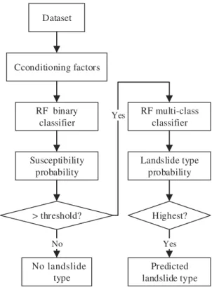
In sum, we need to train a binary RF classifier to predict the landslide susceptibility and train a multi-class RF classifier to infer the landslide type. Given the conditioning factor (input features) of a certain area, we first estimate the susceptibility probability of an

area, if the probability is higher than a predeﬁned threshold, we then predict the most

probable landslide category, as shown on Figure 1. As the RF is the model to do the

binary and multi-class prediction, we mainly describe the RF in the following subsection and then we give a brief introduction to the dataset.

2.1. Random Forest (RF) for landslide susceptibility mapping and classiﬁcation

RF is a data mining algorithm that is able to accurately classify large amounts of data

using an ensemble of decision trees (Breiman, 2001). Decision trees are predictive

models which use a set of binary rules to determine a target variable (Figure 2). The

data used to train the model is comprised of a set of predictor variables and the target variable, which is being predicted. The purpose of the decision tree is to use the predictor variables to partition the data into homogeneous datasets with respect to the target variable. In the simplest case, the target variable will be a binary

classiﬁcation (e.g. the presence or absence of landslides). Both target and predictor

data are present in the root node. The algorithm then tests the ability of each predictor variable to divide the target variable into the two classes. The predictor

(5)

Dataset RF binary classifier RF multi-class classifier Cconditioning factors Highest? Susceptibility probability Landslide type probability Predicted landslide type > threshold? No landslide type No Yes Yes

Figure 1.Predict the susceptibility and landslide type separately.

Root Node Internal node Terminal node Landslide No Landslide Landslide No Landslide Slope > 5° Slope < 5° Lithology = Alluvial Elevation < 100 m Lithology = All others Elevation > 100 m TWI > 11.5 TWI < 11.5 Lithology = Gneiss minuti Lithology = All others Landslide No Landslide Slope > 14° Slope < 14° No Landslide

(6)

variable which leads to the most accurate classiﬁcation is selected and the process is repeated at each of the new nodes. The splitting process continues until there are no more splits to be made (i.e. each terminal node contains target variable data of only a single class).

A single decision tree is a weak classiﬁer. Typically, it has either high variance (the splits at each node are so closely aligned to the training data that the model cannot be used to predict new data) or high bias (the splits do not accurately represent the relationship between predictor and target variables). RF mitigates these problems by using an ensemble of decision trees, which strikes a balance between the two sources of error.

If the same data were used to train multiple decision trees, they would all be identical, which defeats the object of an ensemble model. To avoid this, RF increases

the diversity of the trees by making them grow from diﬀerent sub training datasets

created via bagging. Bagging is used when our goal is to reduce the variance of a decision tree. It generates several subsets of data by randomly sampling with replace-ment from training samples (typically two-thirds) to train multiple decision trees. The rest of the data that is not used to train the decision tree is known as“Out-Of-Bag”(OOB) data. RF further extends the concept of bagging. Besides using the subset of data, it also takes the random selection of predictor variables rather than using all of them to grow trees. The classiﬁcation accuracy of each decision tree and ultimately the RF is assessed

by predicting the mean square error (MSE) of the“out-of-bag”portion of the data, then

averaging over the entire forest (known as the OOB error): MSEOOB¼n1 Xn i¼1ðzi^z OOB i Þ 2 (1) where^zOOB

i is the mean out of bag prediction for theith observation. RF modeling also

provides a measure ofﬁt comparable to theR2values of the other models. This“pseudo

R2”is labeled the“percent variance explained”and is calculated using: Varex¼1 MSEOOB ^ σ2 y (2) where^σ2

yis the total variance of the dependent variable calculated withnas the divisor,

rather thann-1 (Liaw & Wiener,2002).

The OOB data allow RF to rank predictor variables in order of importance. This is done by measuring how much the OOB estimate error increases when data for a particular variable is “removed” from the analysis and the other variables are left intact. This is done on a tree-by-tree basis for the entire forest. The variables which cause the greatest increase in OOB error when removed are deemed to be those of greatest importance.

RF needs to be deﬁned two parameters for generating a classiﬁcation model: the

number of trees in the forest (ntree) and the number of variables tested at each node

(mtry) to make the tree grow. There are no speciﬁc rules about the number of trees

required in a RF and increasing the number of trees does not automatically increase the accuracy of the model, however, it will increase the computational burden. A rule of thumb is that the number of trees should be tested and increased to the point where the OOB error stabilizes. Models can be sensitive to the mtry parameter, as using a greater number of variables at each split will increase the strength of the individual tree but also increase the correlation between trees in the forest. Increasing correlation

(7)

between trees typically increases the error rate in predictions, while increasing the predictive accuracy of individual trees decreases error rate. For this reason, it is necessary to test a number of mtry values.

RF makes predictions by running new data down every tree in the forest. The new

data is assigned a classiﬁcation on the basis of majority vote. The proportion of votes

that a class receives is used to attribute a probability of class membership (Bostrom,

2007). For example, if we are using a RF made up of 100 trees and we are trying to

predict whether a new location is susceptible to landslides we take all the condition-ing factors from that location and feed them into the RF. Based on the splittcondition-ing rules

of each 100 trees, the new data will be classiﬁed as either susceptible or

non-susceptible. If trees classify the new data as susceptible and 25 classify as non-175

susceptible the point will be classiﬁed as susceptible (majority vote) and be given the

susceptible class probability of 0.75.

For LSM, the predictor variables are the conditioning factors and the target variable is the presence or absence of landslides. At each node, a number of conditioning factors

are tested to determine which can most accurately diﬀerentiate between susceptible

and non-susceptible areas. Using the example in Figure 2, the ﬁrst split is above and

below slopes of 5°. Following the right-hand branch of the tree, the next split is based on separating alluvial lithology from all over groups. This creates terminal nodes where all data used to train this decision tree has been split into homogenous“Landslide”and

“No Landslide” groups, based on two splitting rules.

The process of identifying the landslide types is very similar to the binary split of

“landslide” and“no landslide” as described above. The only diﬀerence is that now the target variable (landslide class) is multiclass rather than binary. The purpose of splitting decisions is to create homogenous groups of landslide types. Generally, as there are multiple classes, there will need to be more splits to reach terminal nodes, meaning trees will be bigger. New data are still predicted by a majority vote of all trees in the forest, and the proportion of the votes received represents the probability of class

membership. One diﬀerence is that now the majority votes no longer needs to be the

overall majority. For instance, classes A, B, and C receive 40%, 30%, and 30% of the votes, the data will be classiﬁed as a despite the fact that there is a 60% probability that it does not belong to that class.

2.2. Training data and sampling resolution

Developing a RF model for LSM needs data to train the model and validate its predic-tions. For a LSM, the primary requirement is data that represents both susceptible and non-susceptible areas. Typically, susceptible data is sampled from in and around land-slides identiﬁed by the inventory (Nefeslioglu, Gokceoglu, & Sonmez, 2008).

Non-sus-ceptible areas are taken from areas beyond a buﬀer zone of previous landslides (Park,

Choi, Kim, & Kim,2013) or from areas where landslides are physically unlikely to occur (Gomez & Kavzoglu,2005). Inventory data and data on conditioning factors are usually stored as GIS layers made up of grid cells of a given resolution. Once susceptible and

non-susceptible areas have been identiﬁed, sampling conditioning factors from

corre-sponding spatial locations is a straightforward task using GIS. As data mining models are typically “black box”, meaning it is very diﬃcult to deﬁne the relationship between

(8)

variables, the accuracy of the models needs to be tested. Typically, the total training dataset is split with approximately 70% of samples used to train models and the remainder used for validation.

The physical factors known to control slope stability include slope angle, a range of physical soil properties such as shear resistance and cohesion, hydrological

prop-erties and the inﬂuence of biomass (Vorpahl, Elsenbeer, Märker, & Schröder, 2012).

These data are generally not available at large scale; therefore, it is common to use geomorphological attributes that act as a proxy. There are a huge number of data

which can be used as conditioning factors and there is no deﬁnitive method of

selecting which should be used. While some commonly used conditioning factors,

such as slope and lithology, are widely accepted as inﬂuential, there is debate about

the merits of others (Catani, Lagomarsino, Segoni, & Tofani, 2013). In many cases,

selection will depend on data availability, quality, and theﬁndings of related studies.

Landslide inventories often contain other information, including a classiﬁcation.

This is generally based on the volume of material involved, speed, and type of

movement, as well as the underlying geological conditions Varnes (1978). There is,

however, no single exhaustive taxonomy; they can vary both regionally and nation-ally. The end users of the LSMs will typically be familiar with the classiﬁcation system used in their region.

It is necessary to consider the both the format and resolution at which to represent LSMs, this decision should be focused on the end user. Typically, LSMs are used for

planning purposes, hence the map needs to be of suﬃcient resolution to be ﬁ

t-for-purpose, as well as being easy to interpret for non-specialists. This study will present LSMs at a 100 m resolution grid cell format. In comparison to terrain or slope units, grid cells are more easily aggregated to various administrative boundaries, which can aid

decision making (Trigila et al., 2013). This approach is also more straightforward when

sampling input parameters. Catani et al. (2013) found that a grid size of 50–100 provided the most accurate LSM classiﬁcation, therefore, the input data in this study 240 was dis/ aggregated to a 100 m grid.

3. Case study

3.1. Case study area

To demonstrate the eﬃcacy of RF for LSM and classiﬁcation, the method will be

applied to the case study region of Piedmont, a 25,402 km2region in northwest Italy

(Figure 2). This region is particularly appropriate as since 1950, in Italy alone the economic cost of landslides has been more than 53,249 billion Euros. They have also

caused more than 3500 deaths in the country (Trezzini, Giannella, & Guida, 2013).

Italy has the most infrastructure (in terms of km of roads) and land (in terms of km2)

exposed to landslides within Europe, moreover, Piedmont has been identiﬁed as

being within a landslide “hotspot” (Jaedicke et al., 2014). For this reason we would

like to determine both the susceptibility to landslides and the type of landslides to which an area is susceptible.

(9)

3.2. Landslide inventory

The landslide inventory used in this study is SiFRAP (Sistema Informativo Frane in Piemonte Landslide information system in Piedmont) is a dataset containing 30,439 landslides dating from the early twentieth century to 2006, mapped at a scale of

1:10,000 (Figure 3(b)) (Lanteri & Colombo, 2013). This is an update of the IFFI

(Inventario dei fenomeni franosi in Italia—Inventory of Landslide in Italy) project

(Amanti, Bertolini, & Ramasco, 2001). Of the 30,439 landslides, 236,715 have been

classiﬁed based on the type of mass movement involved (Table 1). A comprehensive

description of the classiﬁcation taxonomy is available from SiFRAP (Piemonte,2009). The location of the landslides in the inventory are shown inFigure 3(b).

3.3. Conditioning factors

A description of some commonly used LSM conditioning factors is shown in Table 2,

along with a description of the ranges of data found in our case study region.

Landslide areas were sampled at a 100 m grid resolution, from within the bound-aries of historic landslides within the inventory. The non-landslide data points were also sampled on a 100 m grid, selected randomly from the within the study area, excluding areas within 200 m of the existing landslide sites. The number of non-landslide points was equal to the number of non-landslide points, give a total of 479,412, divided into a training dataset of 335,740 samples and a test dataset 143,692

Figure 3.(a) Location of Piedmont study area within Italy. (b) Location and classiﬁcation of landslide within the study area.

(10)

samples. As not all the landslides have been categorized, a subset of the 236,715 samples, divided into a training dataset of 165,698 and a validation dataset of 71,016

was used to train and test the classiﬁcation model. The accuracy of the maps

produced will be assessed using a confusion matrix, as recommended by Kavzoglu

et al. (2014). For the RF model, we determined 200 trees to be suﬃcient to produce

stable models, echoing other experimental results (Catani et al., 2013; Lanteri &

Colombo, 2013). After testing, the optimal mtry was determined to be 2 variables

at each split. The models were generated using the “RandomForest”package (Liaw &

Wiener,2002) in the R statistical computing language.

3.4. Results

The LSMs produced by RF are shown inFigure 4. Figure 4(a) shows a binary classiﬁ

ca-tion, where the region is classiﬁed as either susceptible to landslides (black) or not

susceptible to landslides (grey). Figure 4(b) shows landslides susceptibility on a contin-uous scale from high to low. As stated, RF can predict both class and the probability of

class membership.Figure 4(b) shows the probability of memberships to the susceptible/

landslide prone class. Across the region, susceptibility is highest in the mountainous areas in the north, west and south of the region and lowest in the alluvial plain in the centre and east.

Using the test dataset, the recall and precision is 88.41% and 88.66%, respectively and the overall classiﬁcation accuracy of the model is just over 88% (Table 3). This means that over 88% of the test dataset was correctly identiﬁed as being either a landslide area

Table 1.Description of landslide classes in the SiFRAP classiﬁcation.

No. Class Description

1 Crash/roll over The mass moves extremely quickly, mainly in free fall. Material will bounce, roll, and shatter into various sized elements. There is intensive fracturing of the displaced rock.

2 Sliding rotational/ translational

Material moves along one or more surfaces, where the shear strength is exceeded, or within a zone characterized by relatively thin intense shear deformation. Sliding surfaces are visible and can be easily distinguished in moderately sized landslides.

3 Slow dripping Movements are characterized by low speed involving soils that are clay-rich with low water content. Slow dripping landslides typically occur on slopes with a shallow gradient.

4 Fast dripping Fast movements, typically on loosely packed soil with high water content on steep slopes. Generally triggered by heavy rainfall.

5 Complex A movement resulting from a combination of two or more other landslides types. 6 DGPV Slow, complex deformation of rock, with no appreciable continuous failure surface.

Deformation occurs slowly, by a process of differential displacement, that develops over a significant period of time causing a long series of differently orientated joints and planes or deformation of the rock mass concentrated long bands localized at different depths and with different thicknesses.

7 Collapsing/ overturning areas

Sudden movement of large amounts of rock placed on walls or very steep slopes. Movement is characterized by falling and rotation. Often fallen material accumulated at the foot of slopes.

8 Widespread shallow Movement of material of limited thickness triggered by hydrometeorological events characterized by loose soil coverage.

9 Multiple Areas aﬀected by one or more landslides and/or by morpho-structural elements associated with them. These landslides are generally not dated, and often involve entire slopes.

(11)

or a non-landslide area (Figure 4(a)). Results show that the largest source of error comes from landslide prone areas being classiﬁed as non-susceptible. This is to be expected as many on the mountainous regions will be highly susceptible to landslide occurrence despite the lack of previously recorded landslides in the area.

Table 2.geomorphological input data description.

Data Description

Digital elevation model (DEM)

Elevation is commonly used in LSM as it is usually indicative of climatic and vegetation patterns. The DEM used in this study is a 20 m resolution raster showing elevation above sea level. Ranging from 61 to 4615 m.

Slope Slope is the angle formed between any part of the surface of the earth and the horizontal. The angle is a prominent controlling factor on the shear stress experienced by earth and rock mass on a slope. This is on a 20 m grid derived from the DEM ranging between 0° and 87°.

Aspect The aspect of each grid cell will have a bearing on the amount of rainfall and intensity of rainfall it experiences, as well as the amount and intensity of solar radiation. Aspect is defined as the compass direction of a slope. From 0° to 360°,flat areas are assigned−1. Curvature Curvature can be thought of as the slope of a slope. This will affect both stress on the material on the slope and the movement of water across the slope surface. Derived from the DEM on a 20m grid. The values range from−510 to 192.

Proﬁle curvature This is the rate at which the slope gradient changes parallel to the direction of maximum slope. A positive value indicates the cell is part of an upwardly concave slope. A negative value indicates that the slope is upwardly convex. In the study areas this ranges from 295.7 to−192.3.

Plan curvature The slope perpendicular to the direction of maximum slope. A positive value indicates the cell is part of a sidewardly concave slope. A negative value indicates that the slope is sidewardly convex. In the study areas this ranges from 59.9 to 214.5. Parent material

Lithology

Lithology represents the geomechanical properties of bedrock and is a controlling factor in the structural and chemical propertied of soil. This study uses a 1 km raster grid showing the dominant parent material, divided in 12 classes in the region (Van Liedekerke, Jones, & Panagos,2006).

Land form Pennock landform classiﬁcation, divided the study areas into seven classes of three-dimensional landform elements. (Pennock, Zebarth, & De Jong,1987). Landform has been shown to strongly inﬂuence LSM (Schulz,2007).

Topographic wetness index (TWI)

Topographic wetness index represents a hypothetical measure of the accumulation of waterﬂow at any point within a river basin. This can be considered to represent the distribution of soil moisture in the region. This was derived from the DEM on a 100m grid. Values range from 3.9 to 30.4.

Soil classification Soils influence how water moves across the landscape. Some soils are more cohesive, others more prone to erosion. This will affect the conditions which trigger landslides and the type of landslide which occurs. World Reference Base (WRB) soil classification on a 1 km grid, divided in 15 classes in the region (Van Liedekerke et al.,2006). Land cover Represents vegetation and how the land is used, both of which can influence

susceptibility. We use the CORINE land cover map 2006. A 1:100,000 scale land cover map divided into 16 land cover classes in the region, produced by interpretation of Landsat TM and SPOT HRV satellite imagery.

Distance from road Building roads can destabilize slopes, leaving them predisposed to landslides. Furthermore, the vibrations caused by traﬃc can become a triggering mechanism. This was derived from the OpenStreetMap road network map of Italy using a GIS operation to calculate distance from a line. This produced a raster grid of 100 m resolution.

Distance from river

Proximity to the stream network has been shown to inﬂuence susceptibility. Streams have the power to erode soil and apparent material (Gomez & Kavzoglu,

2005). This was derived from a river network map of Italy (available from ISPRA) using a GIS operation to calculate distance from a line. This produced a raster grid of 100 m resolution.

Average annual rainfall

Rainfall is generally considered as a triggering mechanism for landslides, however, it is rarely included in LSM. In an study area this large, the rainfall will be spatially variable and should therefore be considered as a predisposing factor (Catani et al.,

2013). Here the average annual rainfall on a 20 km2_{grid ranging from 684 to} 2640 mm y–1_.

Hydrogeological complex

A classiﬁcation based on hydrogeological formations, which contain similar geological, hydrogeological, productivity, and hydrogeochemical facies. This map is produced by ISPRA at 1:10,000 scale, divided into 11 classes within the region.

(12)

RF can also rank predictor variables in order of importance, based on each of their

relative contribution to the classiﬁcation accuracy of the model.Figure 5 shows that

distance to rivers, TWI and rainfall are all important predictors, whereas, the various

measures of curvature are relatively ineﬀective predictors of the presence or absence

of landslides.

In the SiFRAP dataset, landslides have been divided into the multiple classes shown in

Table 1. Figure 6 shows a RF prediction of the dominant landslide classes distributed across the study area. Using the test dataset, the random forest model is shown to have

an overall classiﬁcation accuracy, recall, and precision of 77.51%, 60.34%, and 77.26%,

respectively. According toTable 4, among all categories, the“crash/roll over” and“fast dripping”landslide have the lowest recall value of 18.45% and 11.41%, respectively. This phenomenon may result from the class-imbalanced data samples, which should be

further considered in the future research. Over 75% (Table 4). The probability of

membership to each landslide class is calculated for each of the points in the testing

Figure 4.Landslide susceptibility of Piedmont. (a) A binary classiﬁcation (b) Probability of landslide. Table 3.Classiﬁcation accuracy of the landslide susceptibility test dataset.

Landslide susceptibility—binary Prediction

Recall Average recall Type Landslide No landslide Total

Observed Landslide 60,592 11,209 71,801 84.39% 88.41% No landslide 5442 66,449 71,891 92.43%

Total 66,034 77,658 143,692

-Precision 91.76% 85.57% - 88.41%

(13)

Figure 5.Ranking of predictor variables used in RF susceptibility model. Crash/rollover Slidingroational/translational Slowdripping Fastdripping Complex DGPV Collapsing/overturning Widespreadshallow Multiple 0 20 40 80 Km (a) (b)

Figure 6. a) The dominant landslide class prediction. b) Areas of high landslides susceptibility (susceptibility >0.5) where the probability of landslide class membership is over 0.5, applying this threshold has been shown to improve overall classiﬁcation accuracy to over 85% (Table 5).

(14)

Table 4. Confusion matrix of landslide classi ﬁ cation. Predicted N = 71,017 Type 1 2 3 4 5 6789 Total Recall Average recall Observed 1 359 39 4 2 171 542 806 18 5 1946 18.45% 60.34% 2 11 3794 174 6 475 1070 173 190 691 6584 57.62% 3 1 259 2000 2 610 419 91 83 84 3549 56.35% 4 5 91 13 60 104 106 123 22 2 526 11.41% 5 28 394 410 3 6348 2394 803 118 81 10,579 60.01% 6 4 100 9 0 400 18,484 1327 3 0 20,327 90.93% 7 36 33 5 3 275 1492 14,476 26 0 16,346 88.56% 8 2 117 233 3 218 335 180 2850 437 4375 65.14% 9 0 108 0 0 1 0 0 256 6419 6784 94.62% Total 446 4935 2848 79 8602 24,842 17,979 3566 7719 71,016 -Precison 80.49% 76.88% 70.22% 75.95% 73.80% 74.41% 80.52% 79.92% 83.16% -Average Precison 77.26% 77.15%

(15)

data. Each point is assigned to the class of with the highest probability, giving the results inTable 4. This means that some points are assigned to a class that they probably do not belong to (e.g. if a point is has a 40% probability of belonging to the collapsing/ overturning class, a 30% probability that it belongs to DGPV and a 30% probability that it belongs to sliding Crash/rollover it will be classified as collapsing/overturning, despite the fact the model shows that there is a 60% probability that this is incorrect). As planners will be most interested in focusing resources in areas that are most likely to be impacted, it is possible to combine the susceptibility and classification maps.Figure 6(b) shows areas of high landslides susceptibility (susceptibility > 0.5) where the probability of landslide class membership is over 0.5, applying this threshold has been shown to improve overall classification accuracy to over 85% (Table 5).

The relative importance of the conditioning variables for landslide classiﬁcation is

shown inFigure 7. Again, that distance to rivers and rainfall are important predictors, as is aspect, while in this instance TWI is the least powerful predictor.

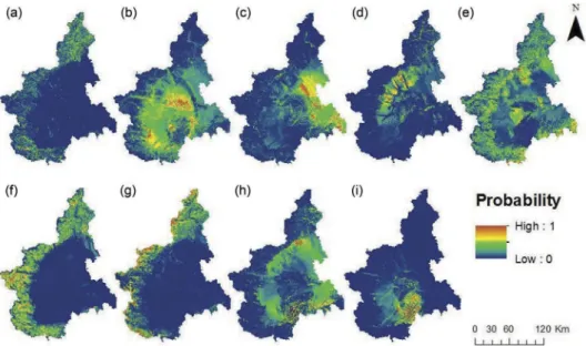
The spatial distribution of the relative probability of each landslide class is shown in

Figure 8. This shows the probability of class membership of each landslide type for every grid cell in the study area. This demonstrates that some landslides, such as collapsing/ overturning and multiple (Figure 8(g,i) respectively) are strongly associated with speciﬁc

regions, whereas others such as sliding rotational/translational (Figure 8(b)) can be

expected in a much greater range of locations. Complex landslides (Figure 8(e)), which

are a combination of two or more other types of landslide have the potential to occur in virtually all locations.

To improve the accuracy of the classiﬁcation, it is possible to impose thresholds so

only points above a set probability are classiﬁed. Increasing the threshold increases the classiﬁcation accuracy (Table 5), however, this approach reduces the number of samples

that can be classiﬁed in the validation dataset (also the amount of the study area that

can be mapped by landslide class).

3.5. Discussion

The RF LSM procedure described in this paper has been shown to be a highly eﬀective way

of predicting and susceptibility and landslide class. Visualising susceptibility and presenting it in a way that can be easily interpreted is a key element of LSM. The rationale is that landslide management strategies have limited resources and should therefore focus on the locations most susceptible to landslides, they also differ depending on the type of land-slides which occur (Guzzetti et al.,1999). Identifying areas that are highly susceptible to landslides is the key issue for those planning mitigation strategies. Knowing the type of landslide that is likely to occur in susceptible regions provides extra information that can improve resource allocation. For ease of interpretation, we suggest a masking process when visualizing results.Figure 6(b) shows landslide classes only for the susceptible areas and only where the probability of class membership is above a 0.5% threshold, this has been shown to improve overall classification accuracy to over 85% (Table 5) and will allow decision makers to focus on highly susceptible and accurately classified areas.

Susceptibility mapping by landslide class (Figure 6(b)) and showing the distribution of landslides types in the study area is a novel approach to LSM. It combines the ease of interpretation provided by multiple maps for individual landslide classes with the

(16)

Table 5.Landslide classiﬁcation accuracy based on probability threshold.

Probability threshold N(validation data) Classiﬁcation accuracy (%)

None 71,016 77.15

0.5 55,359 85.34

0.7 34,869 93.33

0.9 12,989 98.21

Figure 7.Ranking of predictor variables used in RF classiﬁcation model.

Figure 8. Probability of landslide occurrence for each landslide class. (a) Crash/rollover (b) sliding rotational/translational (c) slow dripping (d) fast dripping (e) complex (f) DGPV (g) collapsing/ overturning (h) widespread shallow (i) multiple.

(17)

potential to be incorporated in a generalized hazard assessment (Guzzetti et al.,1999). This method addresses the problem of combining and visualizing the spatial likelihood of multiple types of landslides across a large, heterogeneous region without the need for distinct hazard evaluations. The RF algorithm allows us to predict an overall suscept-ibility across a large, heterogeneous region that experiences a wide range of landslide types without the need for multiple susceptibility analyses. The addition of a classiﬁ ca-tion provides more important informaca-tion which can inform the strategic management of landslide hazards.

The overall classiﬁcation accuracy for the RF LSM (Figure 4) over 88%, which is

favourable compared to other studies using data-mining approaches for LSM which

are typically around 70–80% (Kavzoglu et al., 2014). The case study used is also

substantially larger (at least an order of magnitude) than many others (e.g. (Arnone et al., 2014; Gomez & Kavzoglu, 2005; Pourghasemi et al., 2013; Vorpahl et al., 2012)) suggesting that RF LSM can be applied to heterogeneous landscapes at a regional or national-scale projects.

Of the predictor variables for susceptibility, distance from rivers and TWI are most important. Theseﬁndings contradict those of Catani et al. (2013) who found that neither

TWI nor proximity to rivers were important predictors of landslides. The diﬀerence can

probably be attributed to the diﬀerent landslide inventories and taxonomies, used in

diﬀerent studies. Both TWI and proximity to rivers have been shown to be important

predictors of landslide susceptibility in mountainous regions (Devkota et al.,2013). This seems logical as the majority of landslides in the region occur in mountainous areas, which would coincide with low TWI and larger distances from rivers. This underlines the assertion that empirical LSM models are not readily extrapolated to neighbouring

regions (Guzzetti et al., 1999). This also highlights a limitation of the data-mining

approach, although RF ranks variables in order of importance, there is no way of knowing the process that the variables represent. Nor is there any way of determining

a deﬁnitive ranking of variables as this will depend on the location of the case study,

type of model, resolution of training data, and sampling scheme.

In terms of classiﬁcation, overall, more than three quarters of the test data is classiﬁed

accurately, however, there are substantial diﬀerences between the accuracy of each

class. The accuracy, which is the percentage of the test dataset labelled a certain landslide class in the map is really this class, is all between 70 and 84% accurate. The producer’s accuracy, which is the percentage of a landslide class in the test data being classiﬁed correctly, varies considerably. Only around 18% of the crass/roll over class and

11% of the fast dripping classes are correctly identiﬁed. This may be attributed to the

relative lack of training samples for each class. Many of the crash/rollover landslides have

been classiﬁed as collapsing and overturning or DGPV. This is unsurprising as they have

a similar spatial distribution (Figure 3) and are predicted as occurring in the same areas, associated with high elevation and steep slopes (Figure 8).

onversely, both DGPV and Multiple landslides have over 90% accuracy. Both classes

are strongly associated with speciﬁc, fairly homogeneous spatial regions and have a

relatively high number of samples in the training data, making classiﬁcation more

straightforward. The relative importance of predictors is shown in Figure 7. Distance

from rivers and average annual rainfall are shown as important predictors, as is aspect. Aspect may be a strong predictor as it can be used to distinguish between classes

(18)

associated with low relief, ﬂat areas such as sliding rotational/translational, slow drip-ping, fast dripdrip-ping, and other classes found on the slopes. It may seem unusual that TWI has changed from being a strong predictor of susceptibility to a weak predictor of class, however, this may be due to the clear spatial divide between susceptible and

non-susceptible areas in the study area (Figure 4), which can be linked to low and high TWI

respectively. Within each area, there are a number of classes of landslide, here TWI may have virtually no discriminatory power and lead to misclassiﬁcation.

4. Conclusions and future research

The combination of susceptibility mapping and landslide classiﬁcation using RF is a

novel method which directly addresses the challenges of large-scale LSM in a

region that experiences multiple types of landslides. This study had speciﬁcally

demonstrated that it is possible to use RF to produce highly accurate susceptibility maps for a large heterogeneous region without the need for multiple susceptibility

assessments. Moreover, by joining classiﬁcation and susceptibility predictions, it is

possible to use this method to present planners and decision makers with an LSM that both contains a large amount of information and is easy to interpret. This method can be used to target resources on areas that are highly susceptible to speciﬁc landslides.

Results suggest that there is signiﬁcant scope to develop a joint classiﬁ cation-sus-ceptibility model. Rather than a two-stage modeling process, suscation-sus-ceptibility is deter-mined using a single RF model. The RF is trained to predict landslide classes, with a

further “non-susceptible” class added to the target variables. Research challenges

involved in this approach include how best to sample non-landslide areas and the

number of non-susceptible samples to use in classiﬁcation.

Data availability statement

The data referred to in this paper is not publicly available at the current time.

Acknowledgments

The research has received funding from the European Union’s Seventh Programme for research, technological development and demonstration under grant agreement No 603960—Novel Indicators for identifying critical INFRAstructure at RISK from Natural Hazards (INFRARISKwww. infrarisk-fp7.eu). The third author’s PhD research is jointly supported by China Scholarship Council under Grant 201603170309 and the Dean’s Prize from the University College London.

Disclosure statement

(19)

Funding

The research has received funding from the Seventh Framework Programme, European Union Research and Development Funding Programme for research, technological development and demonstration under grant agreement No 603960—Novel Indicators for identifying critical INFRAstructure at RISK from Natural Hazards (INFRARISK www.infrarisk-fp7.eu). The third author’s PhD research is jointly supported by China Scholarship Council under Grant 201603170309 and the Dean’s Prize from the University College London.

ORCID

Tao Cheng http://orcid.org/0000-0002-5503-9813

References

Akar, Ö., & Güngör, O. (2015). Integrating multiple texture methods and NDVI to the Random Forest classiﬁcation algorithm to detect tea and hazelnut plantation areas in northeast Turkey. International Journal of Remote Sensing,36(2), 442–464.

Alexoudi, M., Manolopoulou, S., & Papaliangas, T. T. (2010). A methodology for landslide risk assessment and management.Journal of Environmental Protection and Ecology,11(1), 317–326. Amanti, M., Bertolini, G., & Ramasco, M. (2001). The Italian landslides inventory–IFFI Project.Paper presented at the Proceedings of III Panamerican Symposium on Landslides, Cartagena, Colombia. Arnone, E., Francipane, A., Noto, L. V., Scarbaci, A., & La Loggia, G. (2014). Strategies investigation in using artiﬁcial neural network for landslide susceptibility mapping: Application to a Sicilian catchment.Journal of Hydroinformatics,16(2), 502–515.

Bostrom, H. (2007). Estimating class probabilities in random forests.Paper presented at the Machine Learning and Applications, 2007. ICMLA 2007, Sixth International Conference on.

Breiman, L. (2001). Random forests.Machine Learning,45(1), 5–32.

Bui, D. T., Tuan, T. A., Klempe, H., Pradhan, B., & Revhaug, I. (2016). Spatial prediction models for shallow landslide hazards: A comparative assessment of the eﬃcacy of support vector machines, artiﬁcial neural networks, kernel logistic regression, and logistic model tree. Landslides,13(2), 361–378.

Catani, F., Lagomarsino, D., Segoni, S., & Tofani, V. (2013). Landslide susceptibility estimation by random forests technique: Sensitivity and scaling issues. Natural Hazards and Earth System Sciences,13(11), 2815–2831.

Cervi, F., Berti, M., Borgatti, L., Ronchetti, F., Manenti, F., & Corsini, A. (2010). Comparing predictive capability of statistical and deterministic methods for landslide susceptibility mapping: A case study in the northern Apennines (Reggio Emilia Province, Italy).Landslides,7(4), 433–444. Clerici, A., Perego, S., Tellini, C., & Vescovi, P. (2006). A GIS-based automated procedure for

landslide susceptibility mapping by the conditional analysis method: The Baganza valley case study (Italian Northern Apennines).Environmental Geology,50(7), 941–961.

Conforti, M., Pascale, S., Robustelli, G., & Sdao, F. (2014). Evaluation of prediction capability of the artiﬁcial neural networks for mapping landslide susceptibility in the Turbolo River catchment (northern Calabria, Italy).Catena,113, 236–250.

Cruden, D. M. (1991). A simple deﬁnition of a landslide.Bulletin of the International Association of Engineering Geology - Bulletin De l’association Internationale De Géologie De l’Ingénieur,43(1), 27–29. Devkota, K. C., Regmi, A. D., Pourghasemi, H. R., Yoshida, K., Pradhan, B., Ryu, I. C., . . . Althuwaynee, O. F. (2013). Landslide susceptibility mapping using certainty factor, index of entropy and logistic regression models in GIS and their comparison at Mugling–Narayanghat road section in Nepal Himalaya.Natural Hazards,65(1), 135–165.

(20)

Epifânio, B., Zêzere, J. L., & Neves, M. (2014). Susceptibility assessment to diﬀerent types of landslides in the coastal cliﬀs of Lourinhã (Central Portugal). Journal of Sea Research, 93, 150–159.

Feng, Q., Liu, J., & Gong, J. (2015). Urbanﬂood mapping based on unmanned aerial vehicle remote sensing and random forest classiﬁer—A case of Yuyao, China.Water,7(4), 1437–1455.

Gomez, H., & Kavzoglu, T. (2005). Assessment of shallow landslide susceptibility using artiﬁcial neural networks in Jabonosa River Basin, Venezuela.Engineering Geology,78(1–2), 11–27. Guzzetti, F., Carrara, A., Cardinali, M., & Reichenbach, P. (1999). Landslide hazard evaluation: A

review of current techniques and their application in a multi-scale study, Central Italy. Geomorphology,31(1), 181–216.

Hengl, T., Heuvelink, G. B., Kempen, B., Leenaars, J. G., Walsh, M. G., Shepherd, K. D., . . . Tamene, L. (2015). Mapping soil properties of Africa at 250 m resolution: Random forests signiﬁcantly improve current predictions.PloS One,10(6), e0125814.

Jaedicke, C., Van Den Eeckhaut, M., Nadim, F., Hervás, J., Kalsnes, B., Vangelsten, B. V., . . . Winter, M. G. (2014). Identiﬁcation of landslide hazard and risk‘hotspots’in Europe.Bulletin of Engineering Geology and the Environment,73(2), 325–339.

Kavzoglu, T., Sahin, E. K., & Colkesen, I. (2014). Landslide susceptibility mapping using GIS-based multi-criteria decision analysis, support vector machines, and logistic regression.Landslides,11 (3), 425–439.

Kumar, D., Thakur, M., Dubey, C. S., & Shukla, D. P. (2017). Landslide susceptibility mapping & prediction using support vector machine for Mandakini River Basin, Garhwal Himalaya, India. Geomorphology,295, 115–125.

Lanteri, L., & Colombo, A. (2013).The integration between satellite data and conventional monitoring system in order to update the Arpa Piemonte landslide inventory Landslide science and practice (pp. 135–140). Berlin: Springer.

Liaw, A., & Wiener, M. (2002). Classiﬁcation and regression by randomForest. R News, 2(3), 18–22.

Mantovani, F., Soeters, R., & Van Westen, C. (1996). Remote sensing techniques for landslide studies and hazard zonation in Europe.Geomorphology,15(3–4), 213–225.

Nefeslioglu, H., Gokceoglu, C., & Sonmez, H. (2008). An assessment on the use of logistic regression and artiﬁcial neural networks with diﬀerent sampling strategies for the preparation of landslide susceptibility maps.Engineering Geology,97(3–4), 171–191.

Park, S., Choi, C., Kim, B., & Kim, J. (2013). Landslide susceptibility mapping using frequency ratio, analytic hierarchy process, logistic regression, and artiﬁcial neural network methods at the Inje area, Korea.Environmental Earth Sciences,68(5), 1443–1464.

Peng, L., Niu, R., Huang, B., Wu, X., Zhao, Y., & Ye, R. (2014). Landslide susceptibility mapping based on rough set theory and support vector machines: A case of the Three Gorges area, China. Geomorphology,204, 287–301.

Pennock, D. J., Zebarth, B., & De Jong, E. (1987). Landform classiﬁcation and soil distribution in hummocky terrain, Saskatchewan, Canada.Geoderma,40(3–4), 297–315.

Piemonte, A. (2009). Guida alla lettura della scheda frane sifrap. Servizio WebGIS Sistema Informativo Frane in Piemonte. Retrieved from http://gisweb.arpa.piemonte.it/arpagis/index. htm

Pourghasemi, H. R., Jirandeh, A. G., Pradhan, B., Xu, C., & Gokceoglu, C. (2013). Landslide suscept-ibility mapping using support vector machine and GIS at the Golestan Province, Iran.Journal of Earth System Science,122(2), 349–369.

Pradhan, B. (2013). A comparative study on the predictive ability of the decision tree, support vector machine and neuro-fuzzy models in landslide susceptibility mapping using GIS. Computers & Geosciences,51, 350–365.

Prasad, A. M., Iverson, L. R., & Liaw, A. (2006). Newer classiﬁcation and regression tree techniques: Bagging and random forests for ecological prediction.Ecosystems,9(2), 181–199.

Regmi, A. D., Devkota, K. C., Yoshida, K., Pradhan, B., Pourghasemi, H. R., Kumamoto, T., & Akgun, A. (2014). Application of frequency ratio, statistical index, and weights-of-evidence models and

(21)

their comparison in landslide susceptibility mapping in Central Nepal Himalaya.Arabian Journal of Geosciences,7(2), 725–742.

Reis, S., Yalcin, A., Atasoy, M., Nisanci, R., Bayrak, T., Erduran, M., . . . Ekercin, S. (2012). Remote sensing and GIS-based landslide susceptibility mapping using frequency ratio and analytical hierarchy methods in Rize province (NE Turkey).Environmental Earth Sciences,66(7), 2063–2073. Schulz, W. H. (2007). Landslide susceptibility revealed by lidar imagery and historical records,

Seattle, Washington.Engineering Geology,89(1–2), 67–87.

Sidle, R. C. (2007). Using weather and climate information for landslide prevention and mitigation. InClimate and land degradation(pp. 285–307). Berlin: Springer.

Taalab, K. P., Corstanje, R., Creamer, R., & Whelan, M. (2013). Modelling soil bulk density at the landscape scale and its contributions to C stock uncertainty.Biogeosciences,10(7), 4691. Tien Bui, D., Pradhan, B., Lofman, O., & Revhaug, I. (2012). Landslide susceptibility assessment in

vietnam using support vector machines, decision tree, and Naive Bayes Models.Mathematical problems in engineering, 2012, Article ID 974638, 26p. doi:10.1155/2012/974638.

Trezzini, F., Giannella, G., & Guida, T. (2013). Landslide andﬂood: Economic and social impacts in Italy. InLandslide science and practice(pp. 171–176). Berlin: Springer.

Trigila, A., Frattini, P., Casagli, N., Catani, F., Crosta, G., Esposito, C., . . . Segoni, S. (2013). Landslide susceptibility mapping at national scale: The Italian case study. InLandslide science and practice (pp. 287–295). Berlin: Springer.

Van Liedekerke, M., Jones, A., & Panagos, P. (2006).ESDBv2 Raster Library-a set of rasters derived from the European Soil Database distribution v2.0 [CDROM]. European Commission and the European Soil Bureau Network, EUR, 19945.

Varnes, D. (1978).Slope movement types and processes—Transportation research board special report. Berlin: Springer.

Varnes, D.J. (1984). IAEG Commission on Landslides and other Mass-Movements Landslide hazard zonation: A review of principles and practice. Paris: UNESCO Press.

Vorpahl, P., Elsenbeer, H., Märker, M., & Schröder, B. (2012). How can statistical models help to determine driving factors of landslides?Ecological Modelling,239, 27–39.

Zare, M., Pourghasemi, H. R., Vafakhah, M., & Pradhan, B. (2013). Landslide susceptibility mapping at Vaz Watershed (Iran) using an artiﬁcial neural network model: A comparison between multi-layer perceptron (MLP) and radial basic function (RBF) algorithms. Arabian Journal of Geosciences,6(8), 2873–2888.

Zêzere, J. (2002). Landslide susceptibility assessment considering landslide typology. A case study in the area north of Lisbon (Portugal).Natural Hazards and Earth System Science,2(1/2), 73–82.