Multiobjective Sparse Ensemble Learning by Means of Evolutionary Algorithms

(1)

Multiobjective Sparse Ensemble Learning by Means of Evolutionary Algorithms

Jiaqi Zhaoa, Licheng Jiaob, Shixiong Xiaa,∗, Vitor Basto Fernandesc,d, Iryna Yevseyevae, Yong Zhoua,

Michael T. M. Emmerichf

a_{School of Computer Science and Technology, China University of Mining and Technology, No 1, Daxue Road, Xuzhou, Jiangsu,} 221116, China

b_{Key Laboratory of Intelligent Perception and Image Understanding of the Ministry of Education, International Research Center} for Intelligent Perception and Computation, Joint International Research Laboratory of Intelligent Perception and Computation,

Xidian University, Xi’an Shaanxi Province 710071, China

c_{Instituto Universit´}_{ario de Lisboa (ISCTE-IUL), University Institute of Lisbon, ISTAR-IUL, Av. das For¸cas Armadas, 1649-026} Lisboa, Portugal

d_{School of Technology and Management, Computer Science and Communications Research Centre, Polytechnic Institute of} Leiria, 2411-901 Leiria, Portugal

e_{Faculty of Technology, De Montfort University, Gateway House 5.33, The Gateway, LE1 9BH Leicester, UK} f_{Multicriteria Optimization, Design, and Analytics Group, LIACS, Leiden University, Niels Bohrweg 1, 2333-CA Leiden, The}

Netherlands

Abstract

Ensemble learning can improve the performance of individual classifiers by combining their decisions. The sparseness of ensemble learning has attracted much attention in recent years. In this paper, a novel multiob-jective sparse ensemble learning (MOSEL) model is proposed. Firstly, to describe the ensemble classifiers more precisely the detection error trade-off(DET) curve is taken into consideration. The sparsity ratio (sr) is treated as the third objective to be minimized, in addition to false positive rate (fpr) and false negative rate (fnr) minimization. The MOSEL turns out to be augmented DET (ADET) convex hull maximization problem. Secondly, several evolutionary multiobjective algorithms are exploited to find sparse ensemble classifiers with good performance. The relationship between the sparsity and the performance of ensemble classifiers on the ADET space is explained. Thirdly, an adaptive MOSEL classifiers selection method is designed to select the most suitable ensemble classifiers for a given dataset.The proposed MOSEL method is applied to well-known MNIST datasets and a real-world remote sensing image change detection problem, and several datasets are used to test the performance of the method on this problem. Experimental results based on both MNIST datasets and remote sensing image change detection show that MOSEL performs significantly better than conventional ensemble learning methods.

Keywords: Ensemble Learning, sparse representation, classification, multiobjective optimization, change detection.

(2)

1. Introduction

The idea of ensemble learning methods [1] is to construct a set of classifiers with base learning al-gorithms and then classify new data points by taking a (weighted) vote of their predictions. Generally, ensemble methods combine the prediction of individual methods and can obtain better predictive perfor-mance than any individual method alone. Ensemble learning methods have attracted much attention in 5

recent years. Not only have many ensemble algorithms been proposed [2, 3], but also ensemble learning methods have been applied to many areas [4, 5], such as medical information processing [1] and satellite image classification [6].

In general, an ensemble learning algorithm is constructed in two steps, i.e., training a number of compo-nent classifiers and then combining the predictions of the compocompo-nents. The most prevailing approaches for 10

training component classifiers are bagging [7], boosting [8], random subspace [9], and rotation forest [10]. Recently, research has drawn attention to multiobjective optimization of ensemble learning [11, 12] and several evolutionary multiobjective algorithms (EMOAs) have been used to deal with it. Generally, most of this work is trying to obtain a set of classifiers with good performance on both diversity and accuracy by using multiobjective optimization algorithms with different objectives. The multiobjective deep belief 15

networks (DBNs) ensemble method was proposed in [13], in which a MOEA was applied to evolve multi-ple DBNs by considering accuracy and diversity as two conflicting objectives. A divide-and-conquer based optimization framework for ensemble classifiers generation was proposed in [12], in which the accuracy of each class was treated as the objectives to describe the performance of classifiers. Besides, maximizing the ensemble size is also taken as an additional objective. The Pareto image features were applied for candi-20

date classifiers generation in [14] by using a multiobjective evolutionary trace transform algorithm. These methods do not consider the redundancy between classifiers and the efficiency of ensemble learning, as it requires a large amount of memory to store the candidates of classifiers and lots of computation time is also needed to predict the label of each new input instance.

In this paper, we focus on combining the predictions of component classifiers by finding several appro-25

priate sparse weight vectors for them. Many works have addressed the complexity of ensemble classifiers by reducing the number of classifiers in the component candidate set. The relationship between the

ensem-∗

Corresponding author. Tel.:+86 051683591709.

(3)

ble learning and its component classifiers is analyzed in [15], which reveals that a better performance can be obtained by ensembling many instead of all the available classifiers. A genetic algorithm is adopted to evolve the weights of the component classifiers, showing that it can generate ensemble classifiers with small 30

sizes but good generalization ability. However, only the accuracy is considered in this method, the result contains redundant classifiers, as the sparsity of ensemble classifiers is not considered. Several pruning strategies are analyzed in [16], including reduction error (RE), Kappa pruning (KP), complementarity mea-sure (CM) and margin distance (MD). Matching pursuit (MP) is used to prune the ensemble classifiers in [17] by balancing the diversity and the individual accuracy.In these methods, the greedy strategy is used to 35

search for the optimal classifiers set and it is easy to fall into the local extremum.

The theoretical and empirical evidence in [18] suggests that a smaller ensemble size can often obtain better performance than a larger ensemble. It is, therefore, possible to obtain an ensemble which mini-mizes the number of individual classifiers and preserves or improves the performance of attributes, such as accuracy and cost of misclassification.

40

Sparse ensembles were proposed in [19]. The outputs of multiple classifiers were combined by using a sparse weight vector. Thehinge lossand the1-normregularization were exploited to calculate the sparse weight vector, formulated as a linear programming problem. However, the1-normmetric cannot describe the sparseness of ensemble classifiers precisely. This is because a weight vector with a group of small values can improve the performance of1-normmeasurement but cannot improve the performance of sparseness. 45

The0-normmetric can describe the sparseness more precisely [20]. The sparse ensemble learning is applied for synthetic aperture radar (SAR) image classification in [6] and for Youtube videos classification in [21]. The0-normlearning can be regarded as an NP-hard problem, it is still an open problem to search the global

optimum.

Compressed sensing (CS) [22] was brought to ensemble learning in [23]. It explores the globally opti-50

mal subset of classifiers for a given ensemble. To solve the compressed sensing problem, a sparse weighting vector which contains many zeros should be generated first, and then appropriate weights should be pro-vided for the remaining classifiers according to their relative importance. Several popular methods such as SpaRAS [24], OMP [25], FISTA [26], PFP [27] are used to tune the weight vector of ensemble classifiers.In [23] it is shown thatcompressed sensing ensembles are often as accurate as, or more accurate than, conven-55

(4)

should be set in advance when using the compressed sensing methods. Meanwhile, the characteristics of the unbalanced data classification were not taken into consideration.

In this paper, we propose the novel concept of a multiobjective sparse ensemble learning (MOSEL) method, in which the relationship between the sparsity and the classification performance is explained. To 60

accurately describe the performance of ensemble classifiers, the detection error trade-off(DET) [28] perfor-mance is taken into consideration by adopting the false positive rate (fpr) and the false negative rate (fnr)

simultaneously. Besides, the sparsity ratio (sr) of ensemble classifiers is treated as the third objective to be minimized. The DET can describe the classifiers more precisely than the accuracy metric especially for unbalance data classification problems [28]. Besides, the evolutionary multiobjective algorithm (EMOA) 65

[29] technique is first applied to evolve the combining weights of ensemble component classifiers. With the technique of tri-objective ensemble learning, we can obtain a set of ensemble classifiers with different sparseness, rather than an ensemble classifier with a certain sparseness that is previously set. The spar-sity and the error rates of ensemble classifiers are explainable and their trade-offs are quantifiable in the augmented DET (ADET) space.

70

We analyze the properties of the ADET for sparse ensemble learning and several state-of-the-art many-objective optimization algorithms are applied to solve multimany-objective ADCH maximization problems, in-cluding the two-archive algorithm (Two Arch2) [30], which focuses on convergence and diversity sepa-rately, the decomposition based algorithms, such as NSGA-III [31], the evolutionary algorithms based on both dominance and decomposition (MOEA/DD) [32], the reference vector guided evolutionary algorithm 75

(RVEA) [33], an indicator based evolutionary algorithm with reference point adaptation (AR-MOEA) [34], and 3D convex-hull-based evolutionary multiobjective optimization algorithm (3DFCH-EMOA) [35, 36]. By using EMOAs we can obtain a set of potentially optimal ensemble classifiers with differentsr-fpr-fnr

trade-offs.

The remaining paper is organized as follows. Section 2 gives a brief introduction to multiobjective 80

optimization of sparse ensemble method. Section 3 presents the results of several classification problems with MNIST [37] and remote sensing change detection datasets, and Section 4 provides concluding remarks.

(5)

2. Multiobjective sparse ensemble learning

2.1. Ensemble Learning

The idea of asparse ensembleof classifiers is to combine the predictions of all classifiers in the candidate 85

set using a sparse weight vector. The sparse vector has many elements with the value of zero and only classifiers corresponding to nonzero weights are selected for the ensemble. To improve the performance of the ensemble classifier and to reduce the memory demand for the components, it is required to select an optimal subset of classifiers and the corresponding weights vector for this subset. The problem of seeking sparse weights vectors can be modeled as a combinatorial optimization problem, which can be solved by 90

evolutionary algorithms [30].

In this paper, we only consider binary supervised ensemble classification problems. With a set of training samplesXtr = {(xj,yj)|xj ∈ Rd,yj ∈ {−1,+1},j = 1,2, . . . ,Mtr}, whereyj is the class label

cor-responding to a given input xj, d is the dimensionality of sample of features, and Mtr is the number of

instances. Note that in this work we only consider binary classification problems and we set the labels as 95

{−1,1}, where 1 represents positive category and−1 represents negative category, given a set of classifiers

{C₁(x),C₂(x), . . . ,CN(x)}, whereCi(x) is thei-th classifier in the candidate ensemble set. Usually, the

clas-sifierCi(x) is obtained by using the training datasetXtrwith the strategy of random selection of the features

or the instances.

A classifier can be obtained by using a training dataset with a machine learning algorithm, which can be 100

described as an estimate of the unknown functiony= f(x). The classifierCi(x) is a hypothesis fi(x) about

the true function f(x), which can predict the class labelyfor a new input vectorxfrom a testing datasetXts

or a validation datasetXval. Usually, the training dataset is used for base classifiers learning, the validation

dataset is used for ensemble pruning and the test dataset is used for ensemble classification performance evaluation. Denote by fjithe prediction of theith learnerCi(x) for the jth sampling of the validation sample

105

xj, that is described by Eq. (1).

fji=Ci(xj). (1)

The prediction output label vectorfican be obtained by implementing the classifierCifor the validation

(6)

fi =[f1i, f2i, . . . , fMvali] T_.

(2)

The matrixFof prediction labels for all instances obtained by all of the classifiers can be denoted by Eq. (3),

110

F=[f1,f2, . . . ,fN] (3)

wheref_i =[f₁i, f2i, . . . , fMi]T,i=1,2, . . . ,N, andF∈RMval×N.

The ensemble learning can improve the performance of classifiers by combining the decisions of each classifier and assigning weightwi to each of the classifierCi(x), and the vector of weightswis denoted by

Eq. (4).

w=[w1,w2, . . . ,wN]T. (4)

The predicted label vectorypredictobtained by ensemble learning for the input datasetXcan be described

115

as in Eq. (5).

ypredict =Fw. (5)

The perfect ensemble classifier can be obtained by solving an equation yval = ypredict. Usually, the

number of equations is larger than that of the weighting variables in the equation system. In this case, there are typically no exact solutions for equations. In this case, the equation system can be approximately solved by using optimization algorithms to find solutions, which can minimize the difference between the training 120

labels and predicting labels.

2.2. Multiobjective optimization of ensemble learning

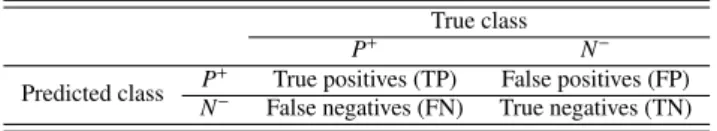
The DET curve [28] is taken into consideration to describe the performance of ensemble classifiers, which has been proved to be a good measurement to evaluate the performance of classifiers [38]. The definition of the DET curve is closely related to the two-by-two confusion matrix, which describes the 125

(7)

is shown in Table 1, which includes four possible outcomes. An outcome is a true positiveif a positive instance is correctly classified and it is atrue negativeif a negative instance is correctly classified. Whenever a negative instance is classified as positive, we call it afalse positive. Finally, whenever a positive instance is classified as negative, we call it afalse negative.

130

Table 1: A two-by-two confusion matrix of binary classifiers True class

P+ N−

Predicted class P+ True positives (TP) False positives (FP)

N− _{False negatives (FN)} _{True negatives (TN)}

Let TN denote the number of true negatives, FP the number of false positives, TP the number of true positives, and FN the number of false negatives. Then the false positive rate (fpr) is defined as fpr =

FP/(TN + FP), and the false negative rate (fnr) is defined as fnr = FN/(TP+ FN). To minimize the difference between true labels and predicted labels, bothfprandfnrshould be minimized.

To obtain sparse ensemble classifiers with good performance, not only should the difference between 135

true label vector yval and predicted label vector ypredict be minimized, but also the number of nonzero

elements in the weight vectorwshould be minimized. In Eq. (6) we define the sparsity ratio (sr) to describe the sparseness of ensemble,

sr= kwk0

N . (6)

Here, N is the number of classifiers in the candidate ensemble set and kwk0 represents the number of

nonzero entities in the weight vector. The weight vectorwis constrained to non-negative values, as negative 140

weightings are neither intuitively meaningful nor reliable [23]. We try to find ensemble classifiers with a low value ofsrin order to reduce classification effort and to counteract overfitting of the ensemble classifier. The computational cost of an ensemble classifier with highsris considered to be higher than that of an ensemble classifier with lowersr. We prefer an ensemble classifier with lowersrwhen given two ensemble classifiers with the same performance criteria (fpr,fnr). Sosr,fprandfnrare conflicting with each other. 145

A low value ofsrmeans that a small number of classifiers are selected for the ensemble, i.e., the ensemble classifier has a low value ofsr, which would result in a poor performance offprandfnr. By treating the sparse termsr as the third objective, the sparse ensemble turns out to be a multiobjective problem. We

(8)

denote it as multiobjective sparse ensemble learning (MOSEL) which is described in Eq. (7),

min MOSEL(w) :=(f pr,f nr,sr)(w),

subject to w∈Ω, (7)

whereΩis the set of all possible weight vectors andwrefers to the weightings with good performance of 150

sparse ensemble classifiers.

2.3. Sparse real encoding

The sparse real encoding strategy is designed to represent the weight vector for the evolutionary algo-rithms, which is an improved version of the real encoding method. The sparse real encoding is constituted by an array of real values in the interval [0, 0.1]. The length of the chromosome is determined by the num-155

ber of candidate classifiers for ensembles. Two strategies are used to modify the real encoding approach for multiobjective sparse ensembles. One is called hard threshold sparse the other is called inequality constraint. Details will be discussed below.

The classifier with a small value of weight in the ensemble learning system does not contribute much to the final decision. In this paper, we ignore the classifiers with small values by adopting a hard threshold 160

strategy. The value of weights smaller than the threshold is set to zero, as described in Eq. (8)

wupdate(i)=            0, ifw(i)< σ w(i), else, (8)

whereσis the hard threshold. In the experimental section, the value is set to 0.05, whereNis the number of candidate classifiers. The sparse real encoding can model the solution of sparse ensemble learning, and then several EMOAs can be applied to evolve the individuals in the population set.

2.4. Adaptive MOSEL classifiers selection

165

The proposed MOSEL can deliver a set of ensemble classifiers, in this part we designed an adaptive selection method to choose the most suitable classifier for a given dataset [39]. Let p(P+) signify the frequency of positive samples and p(N−) denote that of negative samples for a dataset. With an ensemble

(9)

classifier, the risk (R) can be denoted as Eq. 9,

R=λ(FN,P+)·p(P+)· f nr+λ(FP,N−)·p(N−)· f pr, (9) whereλ(FN,P+) is the loss incurred for decidingNegativewhen the true label isPositiveand so isλ(FP,N−). 170

In many real-world problems we can not obtain the label of each sample, however, we can estimate the dis-tributions of a dataset with a predefined classifier, and we denote them as ˆp(P+) and ˆp(N−). Specifically, we do not consider cost-sensitive classification problem in this paper, Eq. 9 can be simplified as Eq. 10:

R= pˆ(P+)· f nr+pˆ(N−)· f pr. (10)

Algorithm 1Adaptive MOSEL classifiers selection (mosel,Xts)

Require: moselis the ensemble classifiers set, the performance of each classifier in ADET space with

Xvalcan be obtained

Ensure: the most suitable ensemble classifier forXts

1: Sett←0 and select a classifieritfrom the solution setmoselrandomly

2: Predict the labels forXtsbyEnCwitand evaluate the dataset distributions ˆpt(P+) and ˆpt(N −₎ 3: t←t+1 4: it ←arg minn_j₌₁pˆt−1(P+)· f nrj+pˆt−1(N−)· f prj 5: ifit =it−1then 6: returnEnCit 7: else 8: Go to step 2 9: end if

The most suitable ensemble classifier can be selected by minimizing the riskR. The adaptive MOSEL classifiers selection algorithm is described in Alg. 1. Firstly, randomly select an ensemble classifier from 175

themoselset, and then evaluate the distributions of the given dataset. Under the evaluated distributions we can select the most suitable ensemble classifier by minimizing Eq. 10. If the selected classifier is the same as the preselected one it can be returned as the most suitable classifier, else go back to Step 2.

2.5. Framework of MOSEL

The description of the framework of MOSEL is given in Alg. 2. Firstly, we train a set of candidate 180

classifiers with Xtr by adopting bagging or random subspace strategies. Secondly, optimize the sparse

(10)

EMOAs. Thirdly, the most suitable ensemble classifiers for Xts can be obtained by adopting adaptive

MOSEL classifiers selection algorithm. Algorithm 2Learning Procedure for MOSEL

1: Training a set of candidate of classifiers withXtr

2: Optimizing the sparse vectorwby using EMOAs withXval

3: Obtain the most suitable ensemble classifier for Xts by using adaptive MOSEL classifiers selection

algorithm

3. Experimental studies 185

3.1. Algorithms involved

In this section, we present the experimental results of the proposed multiobjective sparse ensemble learning methods and then compare the results with the results obtained by two compressed sensing (CS) ensemble methods and two pruning ensemble methods. The sparse ensemble methods in our comparison in-clude SpaRAS [24], OMP [25], which are the most popular methods for solving sparse reconstruction prob-190

lems [23]. The compared pruning methods are Kappa pruning (KP) [16] and ensemble based on matching pursuit (MP) [17]. Several state-of-the-art EMOAs are used to search the solutions of MOSEL, including Two Arch2 [30], NSGA-III [31], MOEA/DD [32], RVEA [33], AR-MOEA [34] and 3DFCH-EMOA [36]. The MNIST [37] and remote sensing change detection datasets are selected to evaluate the performance of the above methods. The strategy of random subspaces [9] is adopted as the dataset manipulation and the 195

classification and regression tree (CART) [40] is used as the base learner. For each mentioned algorithm, 10 independent trials are conducted.

3.2. Parameter setting

The experiment stopping criteria of the six EMOAs are set with a maximum of 30000 function eval-uations. The simulated binary crossover (SBX) and polynomial bit-flip mutation operators are applied in 200

the experiments with crossover probability of pc = 0.9 and the mutation probability of pm = 0.1. The

population size is set to 100 for all EMOAs. All of the experiments were implemented using Matlab code running on an IBM X3650 server with Xeon E5-2600 2.9GHz processors and 32GB memory under Ubuntu 16.04. The details of experiments are described in the following.

(11)

3.3. Experimental results on MNIST datasets

205

3.3.1. Dataset description

The MNIST dataset [37] is widely used for machine learning and pattern recognition methods on real-world data. It contains a training set with 60,000 examples and a testing set with 10,000 examples. Some samples from MNIST dataset are shown in Fig. 1. The handwritten digits have been size-normalized and centered in a fixed-size image (i.e., 28×28). The intensity of each pixel in an image is treated as its features, 210

so the dimensionality of features set for each sample is 784. In this part, we use small amount of examples for training and validation, and the remains for testing.

Figure 1: Samples from MNIST dataset

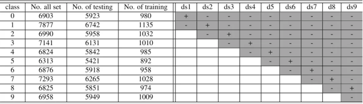
Table 2: The details of MNIST dataset used in the experiments

class No. all set No. of testing No. of training ds1 ds2 ds3 ds4 d5 ds6 ds7 d8 ds9

0 6903 5923 980 + - - - -1 7877 6742 1135 - + - - - -2 6990 5958 1032 - + - - - -3 7141 6131 1010 - + - - - - -4 6824 5842 985 - + - - - -5 6313 5421 892 - + - - -6 6876 5918 958 - + - -7 7293 6265 1028 - + -8 6825 5851 974 - + 9 6958 5949 1009

-The MNIST dataset we used in this part is described in the left part of Table 2. As we only consider binary classification problems in this paper, we select several sub-datasets from the whole dataset, including ds1-ds9 (details are listed in the right part of Table 2). All of the sub-datasets contain two classes, for 215

instance, the positive class in ds2 includes ’1’, and the negative class includes ’0’ and ’2’. Both balanced and unbalanced datasets are created; for instance, in the ds9 dataset, the ratio of positive instances to negative

(12)

instances is about 1:9. For each of the datasets, 1/2 of training instances are randomly selected for candidate classifiers generation and the rest is used for ensemble performance evaluation.

3.3.2. Experimental results and discussion

220

Firstly, the reference Pareto front is shown to illustrate the properties of solutions of tested EMOAs, which is calculated as the best set of solutions of several algorithms achieved in the first experimental run. Without loss of generality, we only discuss the result of the ds3 dataset in Table 2.

0.1 0 0.2 0 0.4 fnr 0.05 sr 0.6 0.8 fpr 1 0.05 0 0.1

(a) The reference Pareto front in 3D

0 0.05 0.1 fpr 0 0.2 0.4 0.6 0.8 1 sr (b)(fpr×sr)projection 0 0.05 0.1 fnr 0 0.2 0.4 0.6 0.8 1 sr (c)(fnr×sr)projection Figure 2: The reference Pareto front for ds3 dataset

The obtained reference Pareto front is shown in Fig. 2(a). We can see that the reference Pareto front includes a set of discrete points on the ADET surface. To illustrate the reference Pareto front clearly, two 225

dimensional projections are shown in Fig. 2(b) and Fig. 2(c), corresponding tofpr×srprojection andfnr×

srprojection, respectively. From Fig. 2(b) we conclude that: 1) Thefprcould not be reduced to zero, even

with all of the classifiers active, but it got very close to it; 2) The best result offprcan be obtained with the

value ofsrin the range of [0.3,0.75] and in the range of [0.75,1.0], which is almost exactly zero; 3) There

are no points (solutions) in the objective space region with the value ofsrbelow 0.3, as the performance of

230

thefpris too bad. From Fig. 2(c) we conclude that: 1) The performance offnrdecreases with the decreasing

ofsr, whensris above 0.8; 2) The best result offnris obtained with the value ofsrin the range of [0.3,0.5];

3) The performance offnris suppressed when the value ofsris below 0.3. Taking the conclusions of Fig.

2 together, some more conclusions can be made: 1) The fpr, fnr andsr are conflicting with each other,

as they cannot reach the best result simultaneously; 2) The highest value ofsr can not guarantee the best 235

performance offpr andfnr; 3) Very few classifiers can reduce the performance of ensemble learning, as

(13)

EMOA are discussed next. 0.1 0 0.2 0 0.4 fnr 0.05 sr 0.6 0.8 fpr 1 0.05 0 0.1

(a) Result of Two Arch2

0.1 0 0.2 0 0.4 fnr 0.05 sr 0.6 0.8 fpr 1 0.05 0 0.1 (b) Result of NSGA-III 0.1 0 0.2 0 0.4 fnr 0.05 sr 0.6 0.8 fpr 1 0.05 0 0.1 (c) Result of MOEA/DD 0.1 0 0.2 0 0.4 fnr 0.05 sr 0.6 0.8 fpr 1 0.05 0 0.1 (d) Result of RVEA 0.1 0 0.2 0 0.4 fnr 0.05 sr 0.6 0.8 fpr 1 0.05 0 0.1

(e) Result of AR-MOEA

0.1 0 0.2 0 0.4 fnr 0.05 sr 0.6 0.8 fpr 1 0.05 0 0.1 (f) Result of 3DFCH-EMOA Figure 3: The Pareto front for ds3 dataset (three axis projection) obtained by six EMOAs

The Pareto front and reference Pareto front by six EMOAs are shown in Fig 3, in which the points of the Pareto front are marked in red and the points of reference Pareto front are marked in blue. By Comparing 240

all Pareto front in Fig 3, we can see that: 1) The solutions of Two Arch2, NSGA-III, MOEA/DD, and AR-MOEA convergence to the local area; 2) The solutions of RVEA and 3DFCH-EMOA are distributed in a wider space; 3) RVEA can find solutions with low value ofsr; 4) 3DFCH-EMOA can obtain solutions with

a high and low value ofsr.

Several metrics are chosen to evaluate the performance of studied algorithms in the comparative exper-245

iment on these datasets, including classification accuracy (acc), false positive rate (fpr), false negative rate

(fnr), sparse ratio (sr) and Kappa coefficient (Kappa) [41]. Kappa coefficient is a statistic indicator which measures inter-rater agreement for categorical items. It is generally thought to be a more robust measure than simple percent agreement calculation, asKappatakes into account the possibility of the agreement

occurring by chance. Generally, the larger the value of theKappa, the better performance of the algorithm. 250

The statistical results of these metrics are listed in the following tables. In these tables the best results obtained are marked in light grey and the second best results are marked in dark grey.

(14)

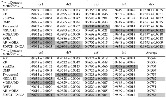
Table 3:Mean and standard deviation of accuracy of ensemble methods on MNIST datasets MethodsDatasets ds1 ds2 ds3 ds4 ds5 MP 0.9889±0.0028 0.9766±0.0023 0.9355±0.0051 0.9419±0.0046 0.9570±0.0035 KP 0.9829±0.0038 0.9695±0.0043 0.9204±0.0046 0.9232±0.0076 0.9503±0.0051 SpaRSA 0.9921±0.0054 0.9836±0.0082 0.9583±0.0201 0.9506±0.0187 0.9741±0.0132 OMP 0.9885±0.0032 0.9765±0.0024 0.9347±0.0043 0.9418±0.0046 0.9561±0.0035 Two Arch2 0.9957±0.0006 0.9891±0.0007 0.9704±0.0016 0.9641±0.0014 0.9787±0.0016 NSGA-III 0.9952±0.0007 0.9893±0.0005 0.9696±0.0021 0.9651±0.0011 0.9798±0.0012 MOEA/DD 0.9952±0.0012 0.9893±0.0009 0.9698±0.0022 0.9644±0.0018 0.9797±0.0010 RVEA 0.9959±0.0008 0.9886±0.0007 0.9696±0.0016 0.9639±0.0015 0.9778±0.0018 AR-MOEA 0.9959±0.0009 0.9897±0.0004 0.9702±0.0015 0.9648±0.0018 0.9795±0.0009 3DFCH-EMOA 0.9962±0.0005 0.9894±0.0005 0.9707±0.0018 0.9654±0.0012 0.9802±0.0013 Methods Datasets _ds6 _ds7 _ds8 _ds9 _Average MP 0.9484±0.0041 0.9714±0.0023 0.9724±0.0018 0.9472±0.0024 0.9599 KP 0.9345±0.0062 0.9622±0.0048 0.9650±0.0048 0.9416±0.0036 0.9500 SpaRSA 0.9624±0.0102 0.9748±0.0123 0.9796±0.0066 0.9578±0.0052 0.9704 OMP 0.9488±0.0043 0.9714±0.0022 0.9726±0.0016 0.9472±0.0024 0.9597 Two Arch2 0.9614±0.0034 0.9830±0.0008 0.9823±0.0006 0.9569±0.0016 0.9757 NSGA-III 0.9638±0.0025 0.9828±0.0006 0.9827±0.0006 0.9579±0.0015 0.9762 MOEA/DD 0.9630±0.0022 0.9829±0.0003 0.9823±0.0007 0.9568±0.0013 0.9759 RVEA 0.9604±0.0020 0.9825±0.0006 0.9820±0.0005 0.9556±0.0013 0.9751 AR-MOEA 0.9619±0.0026 0.9828±0.0006 0.9822±0.0005 0.9569±0.0013 0.9760 3DFCH-EMOA 0.9630±0.0021 0.9832±0.0006 0.9827±0.0004 0.9569±0.0016 0.9764

Table 3 shows the mean and standard deviation of the classification accuracy. The average classification accuracy for each method is listed in the last column of the table. By comparing all the results we can conclude that the methods of MOSEL outperform CS and pruning ensemble methods. 3DFCH-EMOA and 255

NSGA-III outperform other methods for most of the datasets.

Table 4:Mean and standard deviation ofKappaof ensemble methods on MNIST datasets

Methods Datasets _ds1 _ds2 _ds3 _ds4 _ds5 MP 0.9776±0.0056 0.9493±0.0050 0.8214±0.0129 0.8089±0.0159 0.8377±0.0145 KP 0.9657±0.0077 0.9338±0.0092 0.7765±0.0147 0.7474±0.0233 0.8123±0.0184 SpaRSA 0.9841±0.0108 0.9644±0.0177 0.8844±0.0550 0.8395±0.0588 0.9022±0.0491 OMP 0.9769±0.0064 0.9492±0.0051 0.8193±0.0109 0.8088±0.0158 0.8342±0.0136 Two Arch2 0.9914±0.0012 0.9763±0.0016 0.9174±0.0045 0.8805±0.0050 0.9183±0.0065 NSGA-III 0.9903±0.0015 0.9767±0.0012 0.9151±0.0061 0.8844±0.0037 0.9228±0.0047 MOEA/DD 0.9904±0.0024 0.9767±0.0020 0.9159±0.0063 0.8818±0.0062 0.9222±0.0042 RVEA 0.9917±0.0016 0.9751±0.0015 0.9150±0.0046 0.8798±0.0055 0.9147±0.0074 AR-MOEA 0.9917±0.0017 0.9775±0.0009 0.9168±0.0043 0.8832±0.0062 0.9215±0.0035 3DFCH-EMOA 0.9924±0.0011 0.9769±0.0012 0.9182±0.0052 0.8852±0.0043 0.9244±0.0053

MethodsDatasets ds6 ds7 ds8 ds9 Average

MP 0.7539±0.0216 0.8643±0.0104 0.8601±0.0096 0.6601±0.0156 0.8370 KP 0.6718±0.0441 0.8168±0.0256 0.8213±0.0256 0.6243±0.0219 0.7967 SpaRSA 0.8183±0.0453 0.8788±0.0594 0.8965±0.0330 0.7181±0.0269 0.8762 OMP 0.7549±0.0221 0.8645±0.0101 0.8615±0.0083 0.6601±0.0156 0.8366 Two Arch2 0.8060±0.0200 0.9179±0.0038 0.9091±0.0034 0.6993±0.0144 0.8907 NSGA-III 0.8200±0.0144 0.9169±0.0031 0.9112±0.0032 0.7092±0.0134 0.8941 MOEA/DD 0.8155±0.0134 0.9175±0.0018 0.9088±0.0040 0.6989±0.0117 0.8920 RVEA 0.8002±0.0119 0.9156±0.0033 0.9072±0.0029 0.6881±0.0120 0.8875 AR-MOEA 0.8091±0.0156 0.9170±0.0029 0.9087±0.0027 0.7002±0.0114 0.8917 3DFCH-EMOA 0.8149±0.0126 0.9191±0.0032 0.9110±0.0023 0.6991±0.0143 0.8935

(15)

The statistical results of Kappaare shown in Table 4. By comparing the results on the table, we can

see that MOSEL methods outperform CS and pruning methods for most of the MNIST datasets. NSGA-III and 3DFCH-EMOA outperform other methods on most of these datasets. NSGA-III plays slightly better than 3DFCH-EMOA in the metric ofKappa. SpaRSA performs better than other CS and pruning ensemble 260

methods.

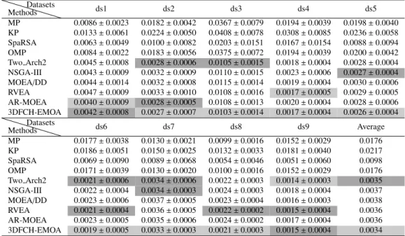
Table 5:Mean and standard deviation offprof ensemble methods on MNIST datasets

MethodsDatasets ds1 ds2 ds3 ds4 ds5 MP 0.0086±0.0023 0.0182±0.0042 0.0367±0.0079 0.0194±0.0039 0.0198±0.0040 KP 0.0133±0.0061 0.0224±0.0050 0.0408±0.0078 0.0308±0.0085 0.0236±0.0058 SpaRSA 0.0063±0.0049 0.0100±0.0082 0.0203±0.0151 0.0167±0.0154 0.0088±0.0094 OMP 0.0084±0.0022 0.0183±0.0056 0.0375±0.0072 0.0194±0.0039 0.0200±0.0042 Two Arch2 0.0045±0.0008 0.0028±0.0006 0.0105±0.0015 0.0018±0.0004 0.0028±0.0004 NSGA-III 0.0043±0.0009 0.0032±0.0009 0.0110±0.0015 0.0023±0.0006 0.0027±0.0004 MOEA/DD 0.0044±0.0014 0.0032±0.0008 0.0115±0.0014 0.0019±0.0004 0.0030±0.0006 RVEA 0.0047±0.0009 0.0033±0.0010 0.0108±0.0016 0.0017±0.0005 0.0029±0.0005 AR-MOEA 0.0040±0.0009 0.0028±0.0005 0.0108±0.0013 0.0020±0.0004 0.0028±0.0006 3DFCH-EMOA 0.0042±0.0008 0.0027±0.0007 0.0103±0.0014 0.0017±0.0004 0.0026±0.0004

As most of the datasets used in this part are large and the distributions of them are unbalance, a small improvement of the accuracy and Kappa can cause many samples to be correctly classified and reduce

misclassification costs greatly. To show the classification performance in more detail, thefpr andfnrare

compared in Table 5 an Table 6, respectively. From these tables, we can see that MOSEL methods out-265

perform other compared methods onfpr, which represents the misclassification ratio of negative instances.

Since in the most of MNIST datasets that we used in this paper, there are far more negative instances than positive samples, the reduction offpr can largely decrease the number of misclassified samples. When

comparing results for thefnr metric, we can also make a conclusion that the proposed MOSEL methods

have great advantages in the MNIST datasets. 270

Table 7 shows the mean value and standard deviation of non-zero classifiers of the ensemble. By com-paring the results we can conclude that KP and OMP have good performance on sparsity, however, they

(16)

Table 6:Mean and standard deviation offnrof ensemble methods on MNIST datasets MethodsDatasets ds1 ds2 ds3 ds4 ds5 MP 0.0141±0.0054 0.0326±0.0068 0.1521±0.0149 0.2126±0.0195 0.1629±0.0277 KP 0.0213±0.0052 0.0449±0.0094 0.2020±0.0296 0.2605±0.0212 0.1847±0.0212 SpaRSA 0.0098±0.0061 0.0278±0.0090 0.1090±0.0363 0.1802±0.0321 0.1142±0.0356 OMP 0.0151±0.0066 0.0326±0.0080 0.1529±0.0149 0.2127±0.0194 0.1674±0.0232 Two Arch2 0.0040±0.0011 0.0253±0.0018 0.0899±0.0056 0.1722±0.0069 0.1168±0.0102 NSGA-III 0.0055±0.0010 0.0239±0.0009 0.0915±0.0073 0.1648±0.0049 0.1104±0.0079 MOEA/DD 0.0052±0.0023 0.0239±0.0020 0.0892±0.0080 0.1700±0.0082 0.1100±0.0069 RVEA 0.0035±0.0014 0.0257±0.0014 0.0925±0.0061 0.1735±0.0084 0.1218±0.0112 AR-MOEA 0.0043±0.0013 0.0237±0.0011 0.0898±0.0061 0.1675±0.0080 0.1116±0.0070 3DFCH-EMOA 0.0032±0.0010 0.0246±0.0009 0.0894±0.0056 0.1657±0.0061 0.1082±0.0084 Methods Datasets _ds6 _ds7 _ds8 _ds9 _Average MP 0.2796±0.0328 0.1403±0.0104 0.1625±0.0138 0.4016±0.0225 0.1731 KP 0.3815±0.0636 0.2011±0.0380 0.2015±0.0309 0.4308±0.0262 0.2143 SpaRSA 0.2445±0.0260 0.1415±0.0526 0.1348±0.0235 0.3857±0.0195 0.1497 OMP 0.2811±0.0324 0.1403±0.0104 0.1600±0.0116 0.4016±0.0225 0.1737 Two Arch2 0.2842±0.0290 0.1140±0.0068 0.1358±0.0053 0.4286±0.0182 0.1523 NSGA-III 0.2652±0.0208 0.1157±0.0052 0.1311±0.0058 0.4149±0.0173 0.1470 MOEA/DD 0.2709±0.0201 0.1127±0.0052 0.1356±0.0058 0.4283±0.0148 0.1495 RVEA 0.2925±0.0176 0.1168±0.0058 0.1383±0.0050 0.4417±0.0158 0.1563 AR-MOEA 0.2792±0.0221 0.1151±0.0069 0.1351±0.0035 0.4264±0.0140 0.1503 3DFCH-EMOA 0.2735±0.0185 0.1127±0.0054 0.1332±0.0041 0.4288±0.0185 0.1488

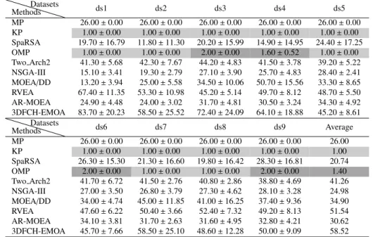
Table 7:Mean and standard deviation of non-zero ensemble weight for each method on MNIST datasets

MethodsDatasets ds1 ds2 ds3 ds4 ds5 MP 26.00±0.00 26.00±0.00 26.00±0.00 26.00±0.00 26.00±0.00 KP 1.00±0.00 1.00±0.00 1.00±0.00 1.00±0.00 1.00±0.00 SpaRSA 19.70±16.79 11.80±11.30 20.20±15.99 14.90±14.95 24.40±17.25 OMP 1.00±0.00 1.00±0.00 2.00±0.00 1.60±0.52 1.00±0.00 Two Arch2 41.30±5.68 42.30±7.67 44.20±4.83 41.50±3.78 39.20±5.22 NSGA-III 15.10±3.41 19.30±2.79 27.10±3.90 25.70±4.83 28.40±2.41 MOEA/DD 13.20±3.94 25.00±5.58 34.50±10.06 50.70±15.56 33.30±8.65 RVEA 67.40±11.35 53.30±10.98 45.20±5.14 49.70±8.12 48.70±5.50 AR-MOEA 24.90±4.48 24.00±3.02 31.70±4.81 30.50±3.24 34.30±4.92 3DFCH-EMOA 83.70±20.23 58.50±25.52 72.40±24.09 64.10±18.88 45.20±8.61

perform poorly on other metrics. If all values in the table are considered, we can conclude that KP has the best sparseness performance. However, the classification accuracy values of OMP and KP are lower than those of MOSEL methods, as these two algorithms do not find good solutions that balance the perfor-275

mance between classification accuracy and ensemble sparsity. As the performance of sparsity and classifi-cation performance are conflicting with each other, a good ensemble method should find the best trade-offs

(17)

between them. From the performed experiments we demonstrate that EMOAs are suitable optimization techniques to tackle sparse ensemble problems.

Table 8:Wilcoxon sum-rank test on MNIST datasets: eachx−y−zin following table means 3DFCH-EMOA winsxtimes, losses

ytimes, drawsztimes

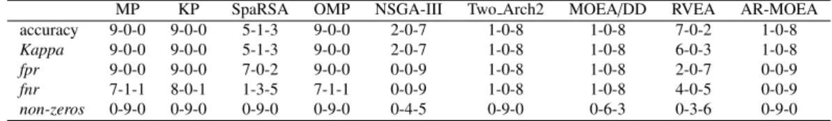
MP KP SpaRSA OMP NSGA-III Two Arch2 MOEA/DD RVEA AR-MOEA

accuracy 9-0-0 9-0-0 5-1-3 9-0-0 2-0-7 1-0-8 1-0-8 7-0-2 1-0-8

Kappa 9-0-0 9-0-0 5-1-3 9-0-0 2-0-7 1-0-8 1-0-8 6-0-3 1-0-8

fpr 9-0-0 9-0-0 7-0-2 9-0-0 0-0-9 1-0-8 1-0-8 2-0-7 0-0-9

fnr 7-1-1 8-0-1 1-3-5 7-1-1 0-0-9 1-0-8 1-0-8 4-0-5 0-0-9

non-zeros 0-9-0 0-9-0 0-9-0 0-9-0 0-4-5 0-9-0 0-6-3 0-3-6 0-9-0

As 3DFCH-EMOA has good performance on most of these datasets, a more comprehensive compari-280

son between 3DFCH-EMOA and other ensemble methods is presented in Table 8, which shows the corre-sponding Wilcoxon sum-rank test [36] results. By comparing the results we can find that 3DFCH-EMOA outperforms CS and pruning ensemble methods significantly on most of the metrics except the non-zeros metric on most of the datasets.

3.4. Experimental results of image change detection

285

Remote sensing image change detection is a real-world problem that aims to find out the change infor-mation that has occurred between two images of the same area taken at different times [42]. It has been applied in many areas, including disaster monitoring, changed target detection and supervision of country resources [43]. Supervised methods have been widely used for remote sensing image change detection [44], as a small amount of labeled data can be used for model training and then the built model can be applied for 290

large-scale image change detection. The change detection problem is an unbalanced classification problem as the proportion of the change area when compared to the total observed area is small. In this part, both synthetic aperture radar (SAR) [45] and optical images are used for the proposed methods evaluation.

3.4.1. Datasets description

Six pairs of remote sensing images are used for classification performance evaluation, details are de-295

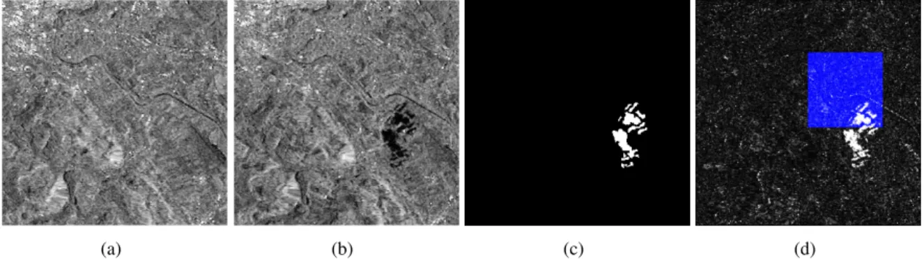
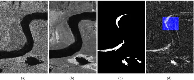
scribed in the following. The first dataset is the Ottawa dataset of two SAR images with a spatial resolution of 10m×10m and a spatial size of 290×350, acquired in July and August 1997, respectively. They were acquired over the city of Ottawa by the Radarsar SAR sensor and were provided by the Defence Research and Development Canada (DRDC)-Ottawa. Fig. 4(a) and (b) present the flood-afflicted areas and Fig. 4(c)

(18)

shows the manually defined reference map. The sample patch for model training and validation is marked 300

in blue with a spatial size 100×100 in the log ratio difference image, as shown in Fig. 4(d).

(a) (b) (c) (d)

Figure 4: Multitemporal images relating to Ottawa. (a) Image acquired in July 1997, during the summer flooding, (b) image acquired in August 1997, after the summer flooding, (c) ground truth, (d) initial difference image obtained via the log ratio operator and examples marked in blue extracted for model training and validation.

The second dataset is the Bern dataset of two SAR images with a spatial resolution of 10m×10m and a spatial size of 301×301. They were acquired over the city of Bern, Switzerland by the European Remote Sensing 2 satellite SAR sensor in April and May 1999, respectively. Fig. 5 shows the two images, manually defined reference map and training image patch with a spatial size 100×100 in the log ratio difference 305

image.

(a) (b) (c) (d)

Figure 5: Multitemporal images relating to the city of Bern. (a) Image acquired in April 1999, (b) image acquired in May 1999, (c) ground truth and (d) examples extracted for model training and validation.

The third dataset is the Mexico dataset of two optical images acquired by Landsat-7 (US satellite) in April 2000 and May 2002, respectively. These two images are extracted from Band 4 of the ETM+images. The sizes of both images are 512×512 pixels. This dataset shows the vegetation damage after the forest

(19)

fire in urban Mexico. Fig. 6(a)-(d) show the two images, reference map and example patch with a spatial 310

size 100×100, respectively.

(a) (b) (c) (d)

Figure 6: Multitemporal images relating to the city of Mexico. (a) Optical image acquired in 2000, (b) optical image acquired in 2002, (c) ground truth and (d) examples extracted for model training and validation.

(a) (b) (c) (d)

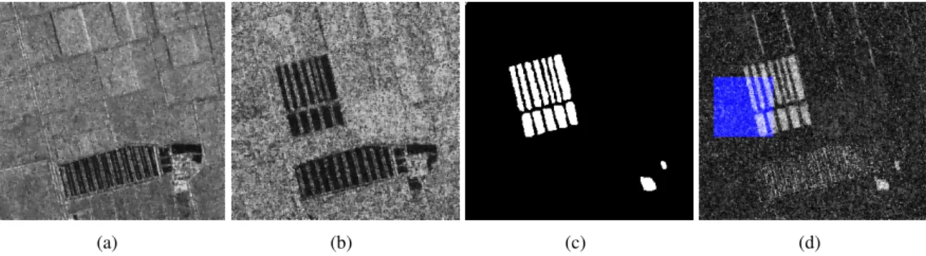
Figure 7: Multitemporal images relating to Farmland of Yellow River Estuary. (a) SAR image acquired in June 2008, (b) SAR image acquired in June 2009, (c) ground truth and (d) examples extracted for model training and validation.

(a) (b) (c) (d)

Figure 8: Multitemporal images relating to Coastline of Yellow River Estuary. (a) SAR image acquired in June 2008, (b) SAR image acquired in June 2009, (c) ground truth and (d) examples extracted for model training and validation.

The 4-6th datasets are the selected from the Yellow River in eastern China of two SAR images cap-tured by Radarsat-2 (Canadian satellite) with a spatial resolution 8m × 8m in July 2008 and June 2009, respectively. Note that the two SAR images are single-look and four-look, respectively, which increases the

(20)

(a) (b) (c) (d)

Figure 9: Multitemporal images relating to Inland water of Yellow River Estuary. (a) SAR image acquired in June 2008, (b) SAR image acquired in June 2009, (c) ground truth and (d) examples extracted for model training and validation.

difficulty of change detection. These datasets include different typical areas, including farmlands, coastline 315

and inland water. Fig. 7 shows the changed areas that appear as newly reclaimed farmlands, with a spatial size 306×291. Fig. 8 shows the coastline where the changed areas are relatively small, with a spatial size 450×280. Inland water where the changed areas are concentrated on the borderline of the river is shown in Fig. 9. The spatial size of Inland water is 291×444.

Table 9: The details of remote sensing datasets Size

Datasets

Ottawa Bern Mexico Farmland Coastline Inland water

Image spatial size 290×350 301×301 512×512 306×291 450×280 291×444 Sample patch size 100×100 100×100 100×100 80×80 80×80 100×100

The spatial and sample patch sizes of these remote sensing dataset are listed in Table 9. In this part, 320

discrete wavelet transform [46], gray-level co-occurrence matrix (CLCM) [47] and Gabor filter bank [6] are selected to extract features for each pixel of log difference images. The dimension of the feature is 38, i.e., each pixel of the log difference image is represented by a 38 dimension vector. For each dataset, 2/3 samples from the training patch are randomly selected for model training and the remaining 1/3 samples are selected for validation. The whole log difference images are used for testing.

(21)

3.4.2. Experimental results and discussion

The mean and standard deviation of the classification accuracy are shown in Table 10. By comparing all the results we can conclude that: 1) OMP performs the best on Ottawa and Farmland datasets; 2) The methods of MOSEL outperform CS and pruning ensemble methods on most of the datasets except Ottawa and Farmland; 3) 3DFCH-EMOA can obtain the highest accuracy except for the Farmland dataset.

330

Table 10:Mean and standard deviation of accuracy of ensemble methods on change detection datasets

Methods Datasets

Ottawa Bern Mexico Farmland Coastline Inland water Average

MP 0.9190±0.0069 0.9880±0.0020 0.9665±0.0043 0.9145±0.0149 0.9855±0.0062 0.9693±0.0027 0.9571 KP 0.8882±0.0657 0.9898±0.0014 0.9670±0.0059 0.9204±0.0154 0.9866±0.0054 0.9659±0.0078 0.9530 SpaRSA 0.9123±0.0235 0.9909±0.0031 0.9636±0.0071 0.9186±0.0108 0.9831±0.0086 0.9677±0.0079 0.9560 OMP 0.9276±0.0023 0.9887±0.0018 0.9682±0.0038 0.9239±0.0050 0.9855±0.0061 0.9694±0.0029 0.9605 Two Arch2 0.9263±0.0027 0.9931±0.0004 0.9725±0.0015 0.9205±0.0020 0.9908±0.0006 0.9731±0.0009 0.9627 NSGA-III 0.9267±0.0030 0.9930±0.0005 0.9723±0.0014 0.9227±0.0034 0.9907±0.0008 0.9735±0.0010 0.9632 MOEA/DD 0.9275±0.0018 0.9932±0.0004 0.9723±0.0014 0.9229±0.0030 0.9911±0.0006 0.9739±0.0010 0.9635 RVEA 0.9262±0.0012 0.9929±0.0004 0.9722±0.0013 0.9206±0.0028 0.9909±0.0006 0.9735±0.0009 0.9627 AR-MOEA 0.9268±0.0025 0.9929±0.0004 0.9716±0.0017 0.9214±0.0040 0.9906±0.0003 0.9734±0.0012 0.9628 3DFCH-EMOA 0.9276±0.0025 0.9934±0.0004 0.9729±0.0014 0.9227±0.0013 0.9911±0.0005 0.9741±0.0007 0.9637

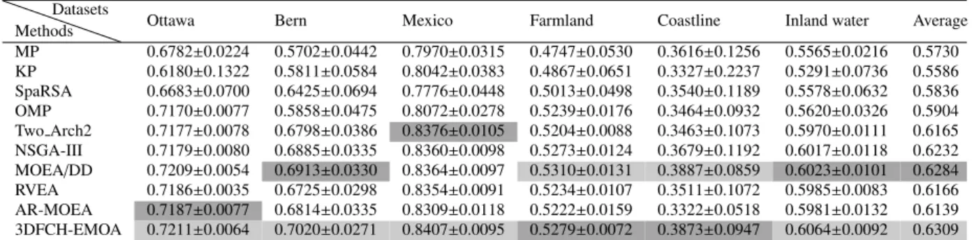
The statistical results of Kappa are shown in Table 11. By comparing the results on the table, we

can conclude that: 1) OMP outperforms other CS and pruning ensemble methods; 2) 3DFCH-EMOA and MOEA/DD perform better than other MOSEL methods on most of the datasets; 3) 3DFCH-EMOA can obtain the best result on the averageKappaof the six remote sensing datasets.

Table 11:Mean and standard deviation ofKappaof ensemble methods on change detection datasets

Methods Datasets

The metrics of fpr and fnr are compared in Table 12 and Table 13, respectively. By comparing the 335

results we can find out that: 1) 3DFCH-EMOA and MOEA/DD perform better than other methods and obtaine lower average offpr, which represents the percentage of unchanged pixels misclassified; 2) SpaRSA

and 3DFCH-EMOA can obtain lower average offnr, which represents the percentage of changed pixels

(22)

good performance on one objective will not have a good performance on another objective. 3DFCH-EMOA 340

can find a good trade-offbetween these two objectives.

Table 12:Mean and standard deviation offprof ensemble methods on change detection datasets

Methods Datasets

Table 13:Mean and standard deviation offnrof ensemble methods on change detection datasets

Methods Datasets

Table 14:Mean and standard deviation of non-zero ensemble weight for each method on change detection datasets

Methods Datasets

Table 14 shows the mean value and standard deviation of non-zero classifiers of the ensemble weight. By comparing the results we can conclude that KP and OMP have good performance on sparsity, however, they perform poorly on accuracy andKappametrics.

As 3DFCH-EMOA has good performance on most of the compared metrics, we make a more compre-345

(23)

Table 15: Wilcoxon sum-rank test on change detection datasets: eachx−y−zin this table means that 3DFCH-EMOA winsx

times, lossesytimes, drawsztimes

MP KP SpaRSA OMP NSGA-III Two Arch2 MOEA/DD RVEA AR-MOEA

accuracy 5-0-1 5-0-1 5-0-1 4-0-2 2-0-4 0-0-6 0-0-6 2-0-4 1-0-5

Kappa 5-0-1 5-0-1 4-0-2 3-0-3 0-0-6 0-0-6 0-0-6 1-0-5 0-0-6

fpr 3-0-3 5-0-1 3-0-3 3-0-3 2-0-4 0-0-6 0-0-6 1-0-5 0-0-6

fnr 3-0-3 2-0-4 3-0-3 3-0-3 0-0-6 0-0-6 0-0-6 0-0-6 1-0-5

non-zeros 0-6-0 0-6-0 0-6-0 0-6-0 0-5-1 0-6-0 0-4-2 0-2-4 0-6-0

results are listed in Table 15. By comparing the results we can find out that 3DFCH-EMOA outperforms CS and pruning ensemble methods significantly on accuracy andKappametrics for most of the datasets.

4. Conclusions

In this paper, we proposed the multiobjective sparse ensemble learning model and analyzed its proper-350

ties in the ADET space. Firstly, MOSEL is modeled as ADCH maximization problem, and the relationship between the sparsity and the performance of ensemble classifiers on the ADET space is explained. Sec-ondly, sparse real encoding is designed as a bridge between MOSEL and EMOAs, and six EMOAs were used to find a sparse ensemble classifier with good performance. Thirdly, an adaptive MOSEL classifier selection algorithm was proposed to select the most suitable ensemble classifier for a given dataset. Exper-355

imental results based on well-known MNIST and remote sensing change detection datasets show that the proposed MOSEL performs significantly better than conventional ensemble learning methods. However, the distribution of MOSEL solutions obtained by several EMOAs is not even. To find evenly distributed solutions MOSEL must be studied further.

Acknowledgment 360

This work was supported by the Fundamental Research Funds for the Central Universities (No. 2018XKQYMS27).

References

[1] S. Piri, D. Delen, T. Liu, H. M. Zolbanin, A data analytics approach to building a clinical decision support system for diabetic retinopathy: Developing and deploying a model ensemble, Decision Support Systems 101 (2017) 12 – 27.

[2] R. Gupta, K. Audhkhasi, S. Narayanan, Training ensemble of diverse classifiers on feature subsets, in: Acoustics, Speech

365

and Signal Processing (ICASSP), 2014 IEEE International Conference on, 2014, pp. 2927–2931.

[3] A. Riccardi, F. Fernandez-Navarro, S. Carloni, Cost-sensitive adaboost algorithm for ordinal regression based on extreme learning machine, IEEE Transactions on Cybernetics 44 (10) (2014) 1898–1909.

(24)

[4] Y. Liu, C. Jiang, H. Zhao, Using contextual features and multi-view ensemble learning in product defect identification from online discussion forums, Decision Support Systems.

370

[5] P. du Jardin, Failure pattern-based ensembles applied to bankruptcy forecasting, Decision Support Systems 107 (2018) 64 – 77.

[6] Z. Zhao, L. Jiao, F. Liu, J. Zhao, Semisupervised discriminant feature learning for SAR image category via sparse ensemble, IEEE Transactions on Geoscience and Remote Sensing 54 (6) (2016) 3532–3547.

[7] L. Breiman, Bagging predictors, Machine Learning 24 (1996) 123–140.

375

[8] J. H. Friedman, Greedy function approximation: A gradient boosting machine., Annals of Statistics 29 (5) (2001) 1189–1232. [9] T. K. Ho, The random subspace method for constructing decision forests, IEEE Transactions on Pattern Analysis and Machine

Intelligence 20 (8) (1998) 832–844.

[10] J. Rodriguez, L. Kuncheva, C. Alonso, Rotation forest: A new classifier ensemble method, IEEE Transactions on Pattern Analysis and Machine Intelligence 28 (10) (2006) 1619–1630.

380

[11] A. Mukhopadhyay, U. Maulik, S. Bandyopadhyay, C. Coello, Survey of multiobjective evolutionary algorithms for data mining: Part II, IEEE Transactions on Evolutionary Computation 18 (1) (2014) 20–35.

[12] M. Asafuddoula, B. Verma, M. Zhang, A divide-and-conquer based ensemble classifier learning by means of many-objective optimization, IEEE Transactions on Evolutionary Computation (2017) 1–1doi:10.1109/TEVC.2017.2782826.

[13] C. Zhang, P. Lim, A. K. Qin, K. C. Tan, Multiobjective deep belief networks ensemble for remaining useful life estimation

385

in prognostics, IEEE Transactions on Neural Networks and Learning Systems 28 (10) (2017) 2306–2318.

[14] W. A. Albukhanajer, Y. Jin, J. A. Briffa, Classifier ensembles for image identification using multi-objective pareto features, Neurocomputing 238 (2017) 316 – 327.

[15] Z.-h. Zhou, J. Wu, W. Tang, Ensembling neural networks: Many could be better than all, Artificial Intelligence 137 (2002) 239–263.

390

[16] G. Mart´ınez-mu¨noz, D. Hern´andez-lobato, A. Su´arez, An analysis of ensemble pruning techniques based on ordered aggre-gation, IEEE Transactions on Pattern Analysis and Machine Intelligence 31 (2009) 245–259.

[17] S. Mao, L. Jiao, L. Xiong, S. Gou, Greedy optimization classifiers ensemble based on diversity, Pattern Recognition 44 (6) (2011) 1245–1261.

[18] H. Chen, P. Tiho, X. Yao, Predictive ensemble pruning by expectation propagation, IEEE Transactions on Knowledge and

395

Data Engineering 21 (7) (2009) 999–1013.

[19] L. Zhang, W.-D. Zhou, Sparse ensembles using weighted combination methods based on linear programming, Pattern Recog-nition 44 (1) (2011) 97 – 106.

[20] L. Li, X. Yao, R. Stolkin, M. Gong, S. He, An evolutionary multiobjective approach to sparse reconstruction, IEEE Transac-tions on Evolutionary Computation 18 (6) (2014) 827–845.

400

[21] Y.-L. Chen, C.-L. Chang, C.-S. Yeh, Emotion classification of youtube videos, Decision Support Systems 101 (Supplement C) (2017) 40 – 50.

(25)

[23] L. Li, R. Stolkin, L. Jiao, F. Liu, S. Wang, A compressed sensing approach for efficient ensemble learning, Pattern Recognition 47 (10) (2014) 3451–3465.

405

[24] S. Wright, R. Nowak, M. Figueiredo, Sparse reconstruction by separable approximation, IEEE Transactions on Signal Pro-cessing 57 (7) (2009) 2479–2493.

[25] G. Davis, S. Mallat, M. Avellaneda, Adaptive greedy approximations, Constructive Approximation 13 (1997) 57–98. [26] K.-C. Toh, S. Yun, An accelerated proximal gradient algorithm for nuclear norm regularized linear least squares problems,

Pacific Journal of Optimization 6 (3) (2010) 615–640.

410

[27] M. D. Plumbley, Recovery of sparse representations by polytope faces pursuit, in: International Conference on Independent Component Analysis and Signal Separation, 2006, pp. 206–213.

[28] A. F. Martin, G. R. Doddington, T. Kamm, M. Ordowski, M. A. Przybocki, The DET curve in assessment of decision task performance, in: European Conference on Speech Communication and Technology, Eurospeech 1997, Rhodes, Greece, September, 1997, pp. 1895–1898.

415

[29] A. Mattiussi, M. Rosano, P. Simeoni, A decision support system for sustainable energy supply combining multi-objective and multi-attribute analysis: An australian case study, Decision Support Systems 57 (Supplement C) (2014) 150 – 159. [30] H. Wang, L. Jiao, X. Yao, Two Arch2: An improved two-archive algorithm for many-objective optimization, IEEE

Transac-tions on Evolutionary Computation 19 (4) (2015) 524–541.

[31] K. Deb, H. Jain, An evolutionary many-objective optimization algorithm using reference-point-based nondominated sorting

420

approach, part I: Solving problems with box constraints, IEEE Transactions on Evolutionary Computation 18 (4) (2014) 577–601.

[32] K. Li, K. Deb, Q. Zhang, S. Kwong, An evolutionary many-objective optimization algorithm based on dominance and decomposition, IEEE Transactions on Evolutionary Computation 19 (5) (2015) 694–716.

[33] R. Cheng, Y. Jin, M. Olhofer, B. Sendhoff, A reference vector guided evolutionary algorithm for many-objective optimization,

425

IEEE Transactions on Evolutionary Computation 20 (5) (2016) 773–791.

[34] Y. Tian, R. Cheng, X. Zhang, F. Cheng, Y. Jin, An indicator based multi-objective evolutionary algorithm with reference point adaptation for better versatility, IEEE Transactions on Evolutionary Computation (2017) 1–1doi:10.1109/TEVC. 2017.2749619.

[35] J. Zhao, V. Basto Fernandes, L. Jiao, I. Yevseyeva, A. Maulana, R. Li, T. B¨ack, K. Tang, M. T.M. Emmerich, Multiobjective

430

optimization of classifiers by means of 3D convex-hull-based evolutionary algorithms, Information Sciences 367–368 (2016) 80–104.

[36] J. Zhao, L. Jiao, F. Liu, V. B. Fernandes, I. Yevseyeva, S. Xia, M. T. Emmerich, 3d fast convex-hull-based evolutionary multiobjective optimization algorithm, Applied Soft Computing 67 (2018) 322 – 336.

[37] Y. Lecun, L. Bottou, Y. Bengio, P. Haffner, Gradient-based learning applied to document recognition, in: IEEE, 1998, pp.

435

2278–2324.

[38] P. Wang, M. Emmerich, R. Li, K. Tang, T. B¨ack, X. Yao, Convex hull-based multi-objective genetic programming for maximizing receiver operator characteristic performance, IEEE Transactions on Evolutionary Computation 19 (2) (2015)

(26)

188–200.

[39] I. Mendialdua, A. Arruti, E. Jauregi, E. Lazkano, B. Sierra, Classifier subset selection to construct multi-classifiers by means

440

of estimation of distribution algorithms, Neurocomputing 157 (2015) 46–60.

[40] X. Wu, V. Kumar, J. R. Quinlan, J. Ghosh, Q. Yang, H. Motoda, G. J. Mclachlan, A. Ng, B. Liu, P. S. Yu, Top 10 algorithms in data mining, Knowledge and Information Systems 14 (1) (2008) 1–37.

[41] G. H. Rosenfield, A coefficient of agreement as a measure of thematic classification accuracy, Photogrammetric Engineering & Remote Sensing 52 (2) (1986) 223–227.

445

[42] M. Gong, J. Zhao, J. Liu, Q. Miao, L. Jiao, Change detection in synthetic aperture radar images based on deep neural networks, IEEE Transactions on Neural Networks and Learning Systems 27 (1) (2016) 125–138.

[43] Y. Zheng, L. Jiao, H. Liu, X. Zhang, B. Hou, S. Wang, Unsupervised saliency-guided sar image change detection, Pattern Recognition 61 (2017) 309 – 326.

[44] R. J. Radke, S. Andra, O. Al-Kofahi, B. Roysam, Image change detection algorithms: a systematic survey, IEEE Transactions

450

on Image Processing 14 (3) (2005) 294–307.

[45] J. Liu, M. Gong, K. Qin, P. Zhang, A deep convolutional coupling network for change detection based on heterogeneous optical and radar images, IEEE Transactions on Neural Networks and Learning Systems 29 (3) (2018) 545–559.

[46] G. Akbarizadeh, A new statistical-based kurtosis wavelet energy feature for texture recognition of sar images, IEEE Transac-tions on Geoscience & Remote Sensing 50 (11) (2012) 4358–4368.

455

[47] B. Hou, X. Zhang, N. Li, Mpm sar image segmentation using feature extraction and context model, IEEE Geoscience & Remote Sensing Letters 9 (6) (2012) 1041–1045.