business.monash.edu/cdes
ABN 12 377 614 012 CRICOS Provider No. 00008C
Centre for Development Economics and Sustainability
Working Paper 01/17
Distribution-sensitive
multidimensional poverty
measures with an
application to India
Gaurav Datt
Abstract
This paper presents axiomatic arguments to make the case for distribution-sensitive
multidimensional poverty measures. The commonly-used counting measures violate
the strong transfer axiom which requires regressive transfers to be unambiguously
poverty-increasing and they are also invariant to changes in the distribution of a given
set of deprivations amongst the poor. The paper provides axiomatic justification for
distribution-sensitive multidimensional poverty measures by appealing to the strong
transfer axiom as well as an additional crossdimensional convexity axiom. Given the
nonlinear structure of these measures, the paper also shows how the problem of an
exact dimensional decomposition can be solved using Shapley decomposition methods
to assess dimensional contributions to the poverty measures. An empirical illustration
for India highlights distinctive features of the distribution-sensitive measures.
Gaurav Datt
Centre for Development Economics and Sustainability, Monash Business School, Melbourne Victoria, Australia
© 2017 Gaurav Datt.
1
Distribution-sensitive multidimensional poverty measures
1. Introduction
Recent estimates suggest that globally about 1.5 billion people live in multidimensional poverty (UNDP, 2015). Over the last decade or so, there has been a veritable explosion of literature on the measurement of multidimensional poverty. Following the initial Atkinson and Bourguignon (1982) paper and important later contributions of Tsui (2002), Bourguignon and Chakravarty (2003) and Alkire and Foster (2007, 2011a), the literature on both the theory and applications of multidimensional poverty measurement has grown rapidly.1 With
regards to applied work, measures within the “counting” approach2 have been influential, in
particular the class of measures proposed by Alkire and Foster (2011a). One indicator of this influence is the publication of the Multidimensional Poverty Index (MPI) – which is a special case of the Alkire-Foster (hereafter AF) class of measures – for more than a 100 countries in the UNDP’s annual Human Development Report since 2010 (UNDP, 2010).3
This influence is only likely to grow with the recent adoption by the UN of the new set of Sustainable Development Goals (SDGs) which encompass a wide range of welfare dimensions many of which are also central to multidimensional poverty measurement.4
This paper revisits the measurement of multidimensional poverty from an axiomatic perspective, taking the AF measures as a point of departure. At its core, it presents
axiomatic arguments for a class of “distribution-sensitive” measures. The arguments centre on the specific formulation of the dominance axioms5, in particular, the transfer and the
rearrangement axioms. The paper proposes stronger versions of these dominance axioms – a stronger version of the transfer axiom requiring regressive transfers (defined later) to be
1 For two recent reviews of the large literature, see Alkire et al (2015) and Aaberge and Brandolini (2015). Also
see Kakwani and Silber (2008).
2These refer to measures that have “tended to concentrate on counting the number of dimensions in which
people suffer deprivation” (Atkinson, 2003, p. 60). See Atkinson (2003) for a distinction between the counting and social welfare approaches to measuring multidimensional deprivation and a common framework within which social judgements inherent to multidimensional poverty comparisons can be considered under the two approaches.
3 Also see a series of Oxford Poverty and Human Development Initiative (OPHI) working and research papers
for a wide range of applications of the AF methodology for countries in Latin America, Sub-Saharan Africa and Asia.
4 Indeed, global MPI has been proposed as a key summary statistic to monitor progress on the SDGs (OPHI,
2014; SDSN, 2014).
5The term “dominance axioms” appears in Foster (2005) and relates to a subset of axioms underlying poverty
2
poverty-increasing, while also introducing a cross-dimensional convexity axiom requiring multiple deprivations to matter more than the sum of their parts, which is shown to be equivalent to a stronger version of the rearrangement axiom.
Two central ideas underlie this paper and the distribution-sensitive measures: (i) regressive transfers in any single dimension reduce social welfare6, and (ii) multiple deprivations have
compounding negative effects on individual and social welfare. The first has a long pedigree in the uni-dimensional poverty literature (see Sen, 1976, for instance) and there are no compelling reasons to eschew it in a multidimensional setting. The second is specific to the multidimensional context, and refers to the cumulative effects of multiple disadvantage on the severity of poverty, whereby the effect of disadvantage in one dimension is exacerbated by disadvantage in another. Multiple disadvantage can thus make it harder to graduate out of poverty. Recent evidence from Banerjee et al. (2015) on the success of multi-faceted interventions in tackling ultra-poverty lends support to the notion of multiple disadvantage as poverty traps. Hence, from this perspective, measures that disregard the extra burden of multiple deprivations could miss out on an important feature of the hardship experienced by those thus deprived.
The paper shows that poverty measures that are inclusive of all deprivations (union-based) and allow for the extra burden of multiple deprivations are distribution-sensitive in two respects: first, they satisfy the strong transfer axiom, and second, they are sensitive to inequality in the distribution of deprivations. The positive contribution of the paper is in bringing these two central ideas together to make a case for this class of distribution-sensitive multidimensional poverty measures which also satisfy a range of other desirable axioms proposed in the literature, without imposing any additional data requirements for practical applications.7
A property of multidimensional poverty measures that has been found to be attractive from a practical and policy perspective is that of dimensional decomposition (sometimes also referred to as factor decomposition), i.e. the ability to decompose the poverty measure into mutually exclusive and exhaustive contributions of each of the included dimensions. The AF measures, for instance, allow for a simple linear decomposition by dimension once the poor
6 Poverty measures can be viewed as a special class of social welfare functions where welfare of the non-poor
is accorded zero weight; see Deaton (1997), for instance, for such an interpretation.
7 There are precursors to this class of measures in the literature in Bourguignon and Charavarty (2003),
Chakravarty and D’Ambrosio (2006) and Alkire and Foster (2011a) – in that the particular mathematical
functional form for the distribution-sensitive measures has been anticipated in these papers, though mainly in passing without exploring the special value of such measures in incorporating distributional considerations as discussed in this paper.
3
have been identified. However, this facility of linear decomposition is no longer available for distribution-sensitive poverty measures when they allow for compounding effects of
deprivations across multiple dimensions. Another contribution of the paper is to show how an exact dimensional decomposition can be implemented in this case drawing upon the Shapley decomposition methods proposed by Shorrocks (2013). The Shapley
decompositions are quite general and can be readily applied to any multidimensional poverty measure, including the AF measures.8 They also have the advantage of fully accounting for
the contributions of dimensions both through the identification of the poor and the aggregation of their individual poverty levels.
The paper presents an application for India to illustrate key properties of
distribution-sensitive poverty measures and how they compare with the AF class of measures. Besides presenting results on the implementation of Shapley dimensional decompositions, the application highlights several ways in which the use of distribution-sensitive measures could matter for measurement and analysis. First, it illustrates how much of multidimensional poverty could be potentially missed by measures that are not union-based and rely on a minimum number (or proportion) of deprivations to identify the poor. Second, it shows how the use of distribution-sensitive poverty measures can influence the profile of the poor and subgroup contributions to poverty. Third, it offers an example of how a maximal
concentration of a given set of deprivations, while reflected in higher values of distribution-sensitive measures, can be consistent with a fall in counting measures. Fourth, using a “mean-inequality” type of decomposition, it shows how the contribution of inequality in the distribution of deprivations to distribution-sensitive measures could be assessed.
The paper is organized as follows. Section 2 introduces the multidimensional poverty measurement framework and the Alkire-Foster measures which offer the point of departure for this paper. Section 3 presents the strong transfer axiom and shows how it is violated by the AF class of measures. Building on that, section 4 elaborates the case for union-based multidimensional poverty measures that are inclusive of all deprivations. Section 5 raises the issue of the dispersion of deprivations across individuals to motivate the
cross-dimensional convexity axiom, which is introduced in section 6. Section 6 also presents the distribution-sensitive multidimensional poverty measures and discusses their properties. Section 7 discusses Shapley dimensional decomposition. The application for India using
8 These decompositions methods are computationally intensive, but this is a lesser-order issue in the
present-day context of rapid computing; for instance, a concise STATA code can run through the necessary calculations in a matter of seconds even for large data sets and a large number of dimensions.
4
data from the Third National Family Health Survey for 2005-6 is presented in section 8. The paper ends with some concluding remarks in section 9.
2. The multidimensional framework and the AF measures
To facilitate presentation of the main arguments of this paper, we adopt largely the same notation as in Alkire and Foster (2011a). Thus, for a fixed population of 𝑛 individuals, 𝑦 = [𝑦𝑖𝑗] denotes an 𝑛 × 𝑑 matrix of non-negative achievements of individuals 𝑖 = 1, … 𝑛 in dimensions 𝑗 = 1, … 𝑑. The dimensional cut-offs (or “poverty lines” for each dimension) are denoted by 𝑧𝑗 > 0 such that individual 𝑖 is deprived in dimension 𝑗 if 𝑦𝑖𝑗< 𝑧𝑗, and
non-deprived otherwise. Given 𝑦 and 𝑧𝑗, a 0-1 deprivation indicator function can thus be defined9 as 𝐼𝑖𝑗 = 𝐼(𝑦𝑖𝑗< 𝑧𝑗) and a corresponding 𝑛 × 𝑑 matrix of proportionate deprivations can be defined as 𝑔𝛼(𝑦) = [𝑔
𝑖𝑗
𝛼], where
𝑔𝑖𝑗𝛼 = (1 − 𝑦
𝑖𝑗/𝑧𝑗)𝛼𝐼𝑖𝑗for𝛼 ≥ 0 (1)
An individual can be deprived in none, one or more dimensions. The number of deprived dimensions for individual 𝑖 is denoted by 𝑐𝑖 = ∑𝑑𝑗=1𝐼𝑖𝑗, or equivalently, by the sum of the 𝑖-th row of 𝑔0(𝑦). Thus, 𝑐
𝑖 or 𝑐𝑖/𝑑 could be interpreted as a measure of breadth of deprivations for an individual, while 𝑔𝑖𝑗𝛼 measures the depth or severity of individual deprivation in a specific dimension for 𝛼 > 0. For ease of exposition, we consider each dimension to carry an equal weight. The arguments presented below carry over to the more general case of unequal weights.
A key and innovative feature of the AF methodology is the idea of a dual cut-off to identify the poor. In addition to the dimensional cut-offs, AF define a poverty or cross-dimensional cut-off 𝑘 as the minimum number of dimensions in which an individual must be deprived in order to be deemed poor. Thus, 𝑘 lies between 1 and 𝑑, and individual 𝑖 is considered poor if 𝑐𝑖 ≥ 𝑘. Analogous and in addition to the deprivation indicator, a poverty indicator function can thus be defined as 𝐼𝑖𝑘= 𝐼(𝑐
𝑖 ≥ 𝑘).
9 The notation 𝑣𝑎𝑟𝑖𝑎𝑏𝑙𝑒 = 𝐼(𝑐𝑜𝑛𝑑𝑖𝑡𝑖𝑜𝑛) indicates that the variable equals 1 if the condition is satisfied, 0
5
With this basic construct, Alkire and Foster (2011a) then define the following class of multidimensional poverty measures, 𝑀(𝛼, 𝑘; 𝑦) as10:
𝑀(𝛼, 𝑘; 𝑦) = 1 𝑛∑ ( 1 𝑑∑ 𝑔𝑖𝑗𝛼 𝑑 𝑗=1 ) 𝐼𝑖𝑘 𝑛 𝑖=1 (2)
Later, it will also be useful to represent 𝑀(𝛼, 𝑘; 𝑦) as an average of individual poverty measures, 𝑚𝑖(𝛼, 𝑘; 𝑦𝑖):
𝑀(𝛼, 𝑘; 𝑦) = 1𝑛∑𝑛𝑖=1𝑚𝑖(𝛼, 𝑘; 𝑦𝑖) where 𝑚𝑖(𝛼, 𝑘; 𝑦𝑖) = (1𝑑∑𝑑𝑗=1𝑔𝑖𝑗𝛼) 𝐼𝑖𝑘 (3) Using notation μ(. . ) to denote the mean of a matrix defined as the sum of all its elements of divided by the total number of its elements, 𝑀(𝛼, 𝑘; 𝑦) can also be written as:
𝑀(𝛼, 𝑘; 𝑦) = 𝜇(𝑔𝛼(𝑘; 𝑦)) where𝑔𝛼(𝑘; 𝑦) = 𝑑𝑖𝑎𝑔(𝐼
𝑖𝑘) 𝑔𝛼(𝑦) (4)
and 𝑑𝑖𝑎𝑔(𝐼𝑖𝑘) is a 𝑛 × 𝑛 diagonal matrix with 1 or 0 as its diagonal elements according as person 𝑖 is poor (deprived in 𝑘 or more dimensions) or not. Note that 𝑀(𝛼, 𝑘; 𝑦) can accommodate cardinal or ordinal data on achievements; if all achievements are binary,
𝑀(0, 𝑘; 𝑦) is well-defined. Alkire and Foster (2011a) show that 𝑀(𝛼, 𝑘; 𝑦) satisfies a number of axioms including: decomposability, replication invariance, symmetry, poverty and
deprivation focus, weak monotonicity, dimensional monotonicity, non-triviality, normalization and weak rearrangement for 𝛼 ≥ 0; monotonicity for 𝛼 > 0; and weak transfer for 𝛼 ≥ 1.11
3. The strong transfer axiom
It is now shown that 𝑀(𝛼, 𝑘; 𝑦) violates an elementary form of the transfer axiom which, following Sen (1976), can be stated as the requirement that a transfer from a poorer to a richer person must increase measured poverty. While Sen referred to this axiom in the context of uni-dimensional poverty measures, it can be adapted to the multidimensional context using the following definition of a poorer person and a transfer in a deprived dimension 𝑗′. Person 𝑖′ is poorer than person 𝑖′′ if 𝑐
𝑖′ ≥ 𝑘 (𝑖′ is poor) and 𝑦𝑖′𝑗≤ 𝑦𝑖′′𝑗 for all 𝑗 and 𝑦𝑖′𝑗′ < 𝑦𝑖′′𝑗′ for at least one 𝑗′ ∈ {1, 2, … 𝑑} (𝑖′ has lower achievement than 𝑖′′ in at least one dimension), or in other words, 𝑦𝑖′′ dominates 𝑦𝑖′ (𝑦𝑖′′𝐷𝑦𝑖′). A (multidimensional)
10 The poverty measures 𝑀(𝛼, 𝑘; 𝑦) are also a function of the 𝑗-vector of dimensional cut-offs, 𝑧; however, this
argument is omitted to ease the notation.
6
distribution 𝑦∗ is obtained from 𝑦 by a transfer in a deprived dimension 𝑗′ from individual 𝑖′ to
𝑖′′ if 𝑦𝑖′𝑗′ < 𝑧𝑗′ and 𝑦𝑖∗′𝑗′ = 𝑦𝑖′𝑗′− 𝜆𝑦𝑖′𝑗′ and 𝑦𝑖∗′′𝑗′ = 𝑦𝑖′′𝑗′+ 𝜆𝑦𝑖′𝑗′ for 0 < 𝜆 ≤ 1 , while 𝑦𝑖𝑗∗ =
𝑦𝑖𝑗 for all other (𝑖, 𝑗) ≠ {(𝑖′𝑗′), (𝑖′′, 𝑗′)}. The strong transfer axiom12 in the multidimensional
context can now be stated.
Strong transfer axiom: If 𝑦∗ is obtained from 𝑦 by a transfer in a deprived dimension from a poorer to a richer person, then 𝑀(𝛼, 𝑘; 𝑦∗) > 𝑀(𝛼, 𝑘; 𝑦).
It is useful to distinguish the strong transfer axiom as stated above from the one-dimensional transfer principle (OTP) in Bourguignon and Chakravarty (2003). Despite their deceptive similarity, OTP is more demanding than the strong transfer axiom: the key difference is that OTP does not require 𝑦𝑖′′ to dominate 𝑦𝑖′ but only 𝑦𝑖′𝑗′ < 𝑦𝑖′′𝑗′ for the transfer in dimension
𝑗′to be poverty-increasing or at least poverty non-decreasing. There is however the issue that if 𝑦𝑖′𝑗> 𝑦𝑖′′𝑗 for other dimensions 𝑗 ≠ 𝑗′, then in what respect should person 𝑖′ (the transferor) be considered “poorer” than person 𝑖′′ (the transferee). By requiring 𝑦
𝑖′′ to dominate 𝑦𝑖′, the transfer axiom makes the notion of “poorer”, and hence the notion of a “regressive” transfer, more precise.
The violation of the strong transfer axiom by 𝑀(𝛼, 𝑘; 𝑦) is now demonstrated by an example. Consider the following 3 person 4 dimension case where the matrices of achievements before and after transfer (by person 2 of two-thirds of her achievement in the 3rd dimension
to person 1) are given by:
𝑦 = [15 83 4 𝟕𝟎𝟔𝟎 00 11 7 150 1
] → 𝑦∗= [15 8 𝟏𝟏𝟎 03 4 𝟐𝟎 0 11 7 150 1 ]
Let the dimensional cut-offs be 𝑧 = [10 5 100 1] and 𝑘 = 2. Then, prior to the transfer, this 3-person community has two poor persons (viz., 1 and 2), and person 2 (the transferor) is unambiguously poorer than person 1 (the transferee) as her achievement vector is dominated by person 1’s achievement vector. Post-transfer, person 1 becomes non-poor. The corresponding pre- and post-transfer deprivation matrices are as below:
12 In an earlier version of the paper (Datt, 2013), this axiom was simply referred to as the transfer axiom. The
adjective “strong” is used here to distinguish it from the weak transfer axiom as in Alkire and Foster (2011a),
which is defined in terms of a progressive transfer involving averaging of achievement vectors of two poor persons where the post-transfer achievement matrix are obtained as the product of a bi-stochastic matrix and the pre-transfer achievement matrix, following Kolm (1977). See Appendix 1 for a formal definition of the weak transfer axiom.
7 𝑔𝛼(𝑦) = [ 0 0 (𝟎. 𝟑) 𝜶 1 (𝟎. 𝟕)𝜶 (𝟎. 𝟐)𝜶 (𝟎. 𝟒)𝜶 1 0 0 0 0 ] → 𝑔𝛼(𝑦∗) = [(𝟎. 𝟕)0 𝜶 (𝟎. 𝟐)0 𝜶 (𝟎. 𝟖)𝟎 𝜶 11 0 0 0 0 ]
It is easy to check that 𝑀(𝛼, 𝑘; 𝑦∗) < 𝑀(𝛼, 𝑘; 𝑦) for all values of 𝛼. A regressive transfer in a single dimension can reduce poverty measured by the AF measure, thus violating the strong transfer axiom. The violation occurs even for 𝛼 > 1 because the transfer to the less poor person can not only eliminate a particular deprivation for that person, but it can also make the person non-poor if she was deprived in exactly 𝑘 dimensions prior to receiving the transfer. Extending the example further, it can be seen that if there is a significant mass of people deprived in 𝑘 dimensions, it will often be possible to steadily reduce the AF measure of multidimensional poverty by a series of regressive transfers from poorer persons, even to the point where achievements of these poorer transferors are driven down to zero in several dimensions.
Conversely, it is easy to check that for 𝛼 > 1 the violation will not occur if the recipient remains poor after the transfer. Fundamentally, the violation arises because the “dual cut-off” assigns a zero weight to any deprivations of non-poor persons.
The statement of the problem also suggests an immediate solution: set 𝑘 = 1. This is the so-called union approach to identification whereby a person is considered poor if deprived in at least one dimension.13 It yields the following multidimensional poverty measure:
𝑀(𝛼; 𝑦) = 1 𝑛𝑑∑ ∑ 𝑔𝑖𝑗𝛼 𝑑 𝑗=1 𝑛 𝑖=1 (5)
This is the same as the additive multidimensional extension of the FGT (Foster, Greer, Thorbecke, 1984) measure in Bourguignon and Chakravarty (2003). While Alkire and Foster (2011a) present their dual cut-off measures as a generalization of the
Bourguignon-Chakravarty measure, the generalization comes at a price (most directly, the violation of the strong transfer axiom as above) that we may not want to pay. The case for union-based measures is further elaborated below.
13 As a corollary, it is worth noting that the AF measure will satisfy the strong transfer axiom if the poverty
cut-off is set at the minimum of the dimensional weights, but that effectively makes it the same as the union approach. Alternatively, if the weight for a particular dimension is set equal to the poverty cut-off (such that it is always included), but other dimensions carry lower weights, then the strong transfer axiom will be satisfied
for such “quasi-union” forms only so long as the regressive transfer from the poor involves the always-included
8
4. Making every deprivation count: the case for the union approach
The violation of the strong transfer axiom highlights an inherent tension within the dual cut-off methodology to multidimensional poverty measurement. At one level, the entire
multidimensional poverty measurement agenda is motivated by the professed need to take account of multiple deprivations faced by individuals and the essentiality of these
deprivations. Yet, the cross-dimensional cut-off forces the poverty measure to neglect deprivations of those deficient in fewer than 𝑘 dimensions, no matter how large those deprivations are. An obvious resolution of the tension is achieved by letting every deprivation count, i.e. by using the so-called union approach. It is also possible to give a human rights interpretation to the union approach such that minimum achievement in every dimension is considered a basic human or social right.14 In effect, this is an argument for
essentiality of all deprivations and relates to the notion that an absence of deprivation in all dimensions is needed to truly escape poverty in a multidimensional setting, and measures that disregard some deprivations could miss out an important part of multidimensional poverty.
Alkire and Foster (2011a) briefly consider the union method, but conclude that it is not appropriate in all circumstances. They offer two arguments. First, “deprivation in certain single dimensions may be reflective of something other than poverty”. Second, “when the number of dimensions is large, the union approach will often identify most of the population as being poor… Consequently, a union-based poverty methodology may not be helpful in distinguishing and targeting the most extensively deprived”. For convenience, let’s term these as the mismeasurement argument (what is measured is not “true” deprivation or poverty) and the targeting argument (what is measured is not helpful for targeting). On closer scrutiny, however, neither argument is particularly compelling.
The mismeasurement argument often takes one of three forms: (i) some deprivations may be “fortuitous” (e.g., a self-made millionaire with little or no education, or a wealthy family who tragically lost a child); (ii) some deprivations may be “chosen” by an individual (e.g., a fashion model, actor or someone who practices fasting may choose to have a low BMI); (iii) deprivations in some dimensions may be measured with error. The argument is that the cross-dimensional cut-off offers a way of “cleansing” the data of such fortuitous or chosen deprivations and of measurement error.
14 For such a human-rights representation of social deprivation in the context of multidimensional poverty
9
But the argument is problematic – on several grounds. First, by insisting on a dual cut-off which requires, say, deprivation in at least 3 of the 10 dimensions for a person for any of her deprivations to be counted in the poverty measure, one not only eliminates cases such as a self-made millionaire with no schooling, but also many others with no schooling who may barely escape deprivation in another two dimensions. The latter’s deprivations are legitimate candidates for inclusion in a poverty measure, but will be ignored by a dual cut-off approach exposing it to significant errors of exclusion. It is even arguable that empirically the errors of such exclusion are likely to be larger than the errors of inclusion under the union approach, given the generally much higher density around the poverty line than around the higher end of the distribution. The union approach avoids these errors of exclusion. Put differently, an implicit assumption in the fortuitous-deprivation argument for a dual cut-off is that all
deprivations of an individual must be “fortuitous” if the total number of deprivations for the individual falls short of the poverty cut-off; and it is this assumption that is questionable. Additionally, in examples of the above kind, it is also arguable that the union approach offers a reasonable alternative. If a wealthy family lost a child, and this is the only single
deprivation that this family has experienced amongst a set of, say, 10 equally-weighted deprivations, then the union approach would accord an individual poverty measure of 0.1 to this family, which is only one-fourth the individual poverty measure of a family who lost a child and is also deprived in three other dimensions, or one-tenth of the individual poverty measure for a family deprived in all dimensions. In other words, fewer deprivations appropriately contribute less to poverty under the union approach.
Second, the issue of “chosen” deprivations is equally problematic. A dual cut-off ignores deprivations below the cross-dimensional cut-off, whether chosen or not, exposing it to problems of exclusion as argued above. There is also the point that whether deprivations exist or not is a conceptually distinct issue from whether deprivations are chosen or not. There are some who believe the poor are the authors of their own misery. But, whatever one’s views on that matter, the issue of “choice” and “attribution of responsibility” for poverty must be distinguished from that of the existence of poverty.
In relation to measurement error, while more accurate data are desirable for both the dual cut-off and union approach, it is arguable that the dual cut-off methodology with its implied censoring presents a rather amputative approach to dealing with measurement error. This has several problems. First, all measured deprivations below the censoring threshold are given a zero weight, whether they are measured with error or not. Second, measurement errors are unlikely to be discontinuous at deprivation thresholds such that it is also possible (on account of measurement error) for someone to be deemed non-deprived in a particular
10
dimension when in fact she is.15 With dual cut-off censoring, it is then possible for this
individual to be deemed non-poor, and thus exacerbating the problem by not only ignoring her mismeasured deprivation, but also all her other deprivations too. Third, measurement errors are also likely to differ across dimensions: some dimensions are harder to measure accurately than others. Yet, dual cut-off censoring as a response to measurement error is completely non-specific with respect to dimensions. Fourth, dual cut-off as a response to measurement error also carries the problematic implication that measurement error matters for those with fewer deprivations than the cross-dimensional cut-off, but may be ignored for those with more deprivations. For all these reasons, the dual cut-off approach does not appear to be a methodologically appropriate response to measurement error.
The targeting argument is of a practical and empirical nature. Alkire (2011) gives an example based on the specific implementation of the AF methodology for the
Multidimensional Poverty Index (MPI) constructed for UNDP’s 2010 Human Development Report, where for 32 out of 104 countries the union approach identifies more than 90 per cent of the population as poor (deprived in at least one of 10 dimensions used for the MPI). The union approach is thus deemed to cast the net too wide. However, firstly, it is not clear to what extent this is an issue of the underlying dimensional cut-offs being too high rather than the cross-dimensional cut-off being too low. An “unacceptably high” headcount of the poor could well be an argument for lowering some of the high cut-offs for particular
dimensions (especially those dimensions that yield high one-dimensional headcounts) rather than for raising the cross-dimensional bar 𝑘 to values above 1.
In relation to targeting, it is further useful to note that given subgroup decomposability, the union-based poverty measure can be written as population share (𝑠𝑗)-weighted sum of poverty measures of 𝑑 mutually exclusive groups comprising respectively of those who are deprived in exactly 𝑗 dimensions for 𝑗 = 1, 2, … 𝑑.
𝑀(𝛼; 𝑦) = 𝑠1𝑀(𝛼; 𝑦|𝑐𝑖 = 1) + 𝑠2𝑀(𝛼; 𝑦|𝑐𝑖 = 2) + ⋯ + 𝑠𝑑𝑀(𝛼; 𝑦|𝑐𝑖 = 𝑑) (6)
Thus, if budgetary resources or other considerations do not allow policymakers to target the full set of those facing any deprivation, it is always possible to drill down a union-based poverty measure and focus on subsets of those deprived in multiple dimensions. For
15 This is what Calvo and Fernandez (2012) describe as type-I errors which tend to counteract the possible
upward bias due to type-II errors (incorrectly counting a non-poor individual as poor). The net effect is
generally indeterminate, as also noted by Calvo and Fernandez: “Whether the dual cut-off finally mitigates or
exacerbates the impact of measurement errors remains an empirical issue” (p.10). However, as they also note, the strength of type-I errors will depend in part on the proportion of population who are deprived in fewer dimensions than the cross-dimensional cut-off. Results for the Indian example in section 8 below show that this proportion can be quite large (see Table 1 below).
11
instance, one could start with those deprived all 𝑑 dimensions, then move on to those deprived in 𝑑 − 1 dimensions, and so on. Alternatively, it is possible to define a target group as bottom 𝑥% of the population when individuals are ranked from the poorest to the least poor in terms of their individual poverty levels 𝑚𝑖(𝛼; 𝑦).
An analogous issue also arises in the context of uni-dimensional or income poverty
measurement where, for a given (uni-dimensional) poverty line, the headcount of the poor in some country contexts may be well above what policymakers wish to target. Arguably, a reasonable and common response is not to redefine the poor by altering (lowering) the poverty line but to treat the target group as a subset of the poor; indeed the concept of the “ultra-poor” for instance offers one way of doing this. A similar approach is of course feasible with multidimensional poverty measures; the need to identify a target group does not by itself offer adequate justification for the use of a cross-dimensional cut-off.1617
As against this, one needs to weigh in the potential benefits of the union approach, a significant one of which is the satisfaction of the strong transfer axiom above. In addition, the union-based approach also allows the monotonicity and dimensional monotonicity axioms to be strengthened as below.
Strong monotonicity18: If distribution 𝑦∗ is obtained from 𝑦 by a decrement in any deprived dimension 𝑗′ for any individual 𝑖′ [i.e. there exists an (𝑖′, 𝑗′) such that 𝑦
𝑖∗′𝑗′ < 𝑦𝑖′𝑗′ < 𝑧𝑗′ while
𝑦𝑖𝑗∗ = 𝑦𝑖𝑗 for all other (𝑖, 𝑗) ≠ (𝑖′, 𝑗′)], then 𝑀(𝛼; 𝑦∗) > 𝑀(𝛼; 𝑦).
Note that strong monotonicity implies monotonicity which only requires the
poverty-increasing property of a decrement in achievements to be satisfied if such decrement occurs for those deprived in at least 𝑘 dimensions. Conversely, for 𝛼 > 0, strong monotonicity will be violated by the AF class of measures unless 𝑘 = 1, i.e., the union case.
A further implication of strong monotonicity is also notable: strong monotonicity implies strong dimensional monotonicity.
16 The argument can also be made that in a multidimensional setting there is no compelling reason to focus on
a particular range for the headcount ratio (𝐻), since the latter is not a member of the AF class of measures. For instance, as Alkire and Foster (2011a) note, 𝐻 violates dimensional monotonicity. The elementary
“counting” measure within the AF class is 𝑀0= 𝐻𝐴 where 𝐴 is the average deprivation intensity amongst the
poor. A high 𝐻 need not result in a high 𝑀0, and union-based measures, by also averaging in those with fewer
than 𝑘 deprivations, will be associated with a lower 𝐴 relative to dual cut-off measures.
17 The general problem of targeting is a complex one involving a range of informational, incentive and political
economy issues. For a discussion of some of these, see for instance Besley and Kanbur (1993), Pritchett (2005), Dreze and Sen (2013). A full discussion of these issues is well beyond the scope of this paper.
12
Strong dimensional monotonicity: If distribution 𝑦∗ is obtained from 𝑦 by an increment in a deprived dimension 𝑗′ for any individual 𝑖′ which makes her non-deprived in that
dimension, [i.e. there exists an (𝑖′, 𝑗′) such that 𝑦
𝑖∗′𝑗′ ≥ 𝑧𝑗′ > 𝑦𝑖′𝑗′ while 𝑦𝑖𝑗∗ = 𝑦𝑖𝑗 for all other
(𝑖, 𝑗) ≠ (𝑖′, 𝑗′)], then 𝑀(𝛼; 𝑦∗) < 𝑀(𝛼; 𝑦).
Strong dimensional monotonicity implies dimensional monotonicity (as in Alkire and Foster, 2011a) where the latter restricts the application of the poverty-decreasing property of the removal of a given deprivation to only those deprived in at least 𝑘 dimensions. Strong dimensional monotonicity will be generally violated by the AF class of measures whenever the elimination of a particular deprivation occurs for someone who is deprived in less than 𝑘
dimensions. Such violation is precluded by setting 𝑘 = 1.
Does the violation of strong monotonicity properties matter? A reason for preferring the stronger versions is that they imply the weaker versions but not the converse. The key difference between the two (as noted above) is that the weaker versions restrict monotonicity to only those who are deprived in at least 𝑘 dimensions, while the stronger versions apply monotonicity to those deprived in any dimension. The difference thus comes down to the issue of essentiality of all deprivations. If all deprivations are deemed worthy of inclusion in a poverty measure, as argued above, then it follows that stronger monotonicity properties are appropriate. A decrement in an inclusion-worthy deprived dimension should lead to an increase in measured poverty, rather than no change; weaker versions will end up ignoring the impact of some deprivations.
5. Sensitivity to concentration of deprivations
Another potential issue with the AF class of counting measures is illustrated by returning to our 3-person 4-dimension example. Consider the following two deprivation matrices with
𝜉𝑗 ≫ 0 and 𝑘 = 2: 𝑔𝛼(𝑦) = [(𝝃𝟏) 𝜶 (𝝃 𝟐)𝜶 0 0 0 0 (𝝃𝟑)𝜶 (𝝃𝟒)𝜶 0 0 0 0 ] → 𝑔𝛼(𝑦∗) = [(𝝃0 0 0 0 𝟏)𝜶 (𝝃𝟐)𝜶 (𝝃𝟑)𝜶 (𝝃𝟒)𝜶 0 0 0 0 ]
Thus, achievement matrices 𝑦 and 𝑦∗ are associated with the same combination of deprivations, but while in 𝑦 individuals 1 and 2 share two deprivations each, in 𝑦∗ all four deprivations are experienced by individual 2. Since the means of the two deprivation matrices are the same, 𝑀(𝛼, 𝑘; 𝑦) = 𝑀(𝛼, 𝑘; 𝑦∗) for all values of 𝛼. Thus, the AF class of measures are completely insensitive to how a given set of deprivations is spread across the
13
poor; maximal and minimal concentrations of deprivations are treated alike. This lack of sensitivity to the distribution of a given set of deprivations amongst the poor is similar to the insensitivity of the headcount and poverty gap indices to inequality below the poverty line in a uni-dimensional setting.
The above example illustrates a case where (in moving from 𝑦 to 𝑦∗) there is a change in the joint distribution of achievements but no change in the censored marginal distributions. Yet, such a change in the joint distribution has no effect on the AF measures19, rendering them,
ironically, somewhat similar in that respect to indices such as the Human Development Index (HDI) or the Human Poverty Index (HPI) which depend only on the marginal distributions of indicators they aggregate.20 Strictly, the joint density across dimensions matters for the AF
measures at the identification stage (in determining whether someone is poor or not), but not at the aggregation stage. Put differently, the AF measures depend on the censored
marginal distributions, and that renders them insensitive to greater or lesser concentration of a given set of deprivations amongst the poor so long as the set of poor remains the same. It is notable that this issue persists even in the union case when 𝑘 = 1 and there is no censoring. In general, 𝑀(𝛼; 𝑦) will be unchanged for any rearrangement of a given set of deprivations for all values of α. In this respect, the AF class of measures (including the special union case with 𝑘 = 1) are rather utilitarian in their reliance on a “sum-ranking” 21, i.e.,
the aggregation of individual deprivations by summing them up.
It is arguable however that a given deprivation is more burdensome for an individual if also accompanied by deprivation in other dimensions. A similar view is echoed by Stiglitz, Sen and Fitoussi (2009, p. 15) in their discussion of measures of the quality of life: “…the
consequences for quality of life of having multiple disadvantages far exceed the sum of their individual effects”. The notion of compounding negative effects of multiple disadvantages is also deeply rooted in the sociological concept of the underclass (e.g. Wilson, 1987, 2006), in
19 This statement on the invariance of AF measures to such changes in joint distribution relates to 𝑀(𝛼, 𝑘; 𝑦)
measures, and not to partial indices, such as 𝐻 and 𝐴, which indeed do not satisfy many of the (axiomatic) properties proposed for the AF measures. For instance, it is true that in the example above, in moving from distribution 𝑦 to 𝑦∗, while poverty incidence, 𝐻, is halved, the intensity of poverty amongst the poor, 𝐴, doubles, which is why the product 𝐻𝐴 = 𝑀(0, 𝑘; 𝑦 remains unchanged. But that only highlights the key issue. As the halving of 𝐻 is a desirable change and the doubling of 𝐴 is the opposite, how do we form a judgement on the overall change? The judgement implicit in the AF measures 𝑀(𝛼, 𝑘; 𝑦), that these two effects always exactly cancel each other out, is contentious. As argued below, the distribution-sensitive 𝑀(𝛼, 𝛽; 𝑦) measures for 𝛽 > 1 incorporate the alternative judgement that the same set of deprivations if shared more (less) equally imposes a lesser (greater) burden on society.
20 This feature of the HDI or HPI is well-known and indeed has been an important motivation for the
development of multidimensional poverty measures (see, for example, Alkire and Foster, 2011b).
14
policy discussions of social exclusion (e.g. Levitas et al, 2007),22 as well as in some
formulations of “poverty traps” (e.g. Durlauf, 2006; Banerjee and Duflo, 2011).23 Common to
these diverse perspectives is the idea that through various mechanisms multiple disadvantages can reinforce each other in the social reproduction of poverty for certain groups, in undermining the long-term “life chances” of the underclass or the future prospects for the most disadvantaged in society. It should scarcely require any convincing that an accumulation of deprivations can be catastrophic to the point of threatening the very survival of individuals or families; all of us know of or have heard or read about one or more cases where such catastrophes have (sadly) eventuated.24
One may also refer to recent evidence from Banerjee et al (2015) on the evaluation of randomized control trials in six countries25 of a multifaceted program aimed at helping the
ultra-poor graduate out of poverty. The program used a holistic approach combining the transfer of a productive asset with consumption support, health and/or education services, training and coaching plus savings encouragement. Banerjee et al. note that “the thinking behind the program is that the combination of these activities is necessary and sufficient to obtain a persistent impact on a large fraction of the beneficiaries” (p. 1260799-1). While they do not test whether each program dimension was individually necessary, their results on the sustained positive impacts on consumption, household assets and food security do offer evidence on the sufficiency claim, consistent with the notion of a big push being able to alleviate the multiple constraints that may keep households trapped in poverty.
6. Cross-dimensional convexity and distribution-sensitive poverty measures It is thus eminently arguable that the concentration or dispersion of deprivations across individuals matters, and a case can be made for the requirement that multidimensional poverty measures be sensitive to the distribution of a given set of deprivations. This can be achieved by requiring the individual multidimensional poverty measure to be convex over individual deprivations in different dimensions, and can be axiomatized as follows.
22 For instance, Levitas et al (2007) drawing upon Miliband (2006) define “deep exclusion” as “exclusion across
more than one domain or dimension of disadvantage, resulting in severe negative consequences for quality of life, well-being and future life chances”.
23 Banerjee and Duflo (2011) give several examples of how interlocking deprivations in multiple dimensions can become “a mechanism for current misfortunes to turn into future poverty”.
24 A large part of the excess mortality in developing countries could arguably be viewed as the consequence of
accumulated multiple deprivations amongst their populations.
25 The six countries include: Ethiopia, Ghana, Honduras, India, Pakistan, and Peru (Banerjee et al 2015). For
related evidence on a multifaceted program targeting ultra-poor women in Northern Kenya, also see Gobin, Santos and Toth (2016).
15
Cross-dimensional convexity: An increment in deprivation 𝑗′ for individual 𝑖 induces a greater increase in measured poverty for individual 𝑖, the greater individual 𝑖’s deprivation in any other dimension 𝑗 ≠ 𝑗′.26
There is no real mystery to the idea that if you are hurting on many fronts, an additional blow could be completely crushing. The cross-dimensional convexity axiom appeals to this idea of the compounding (negative) effect of multiple deprivations on the overall well-being of the individual. It asserts that the severity of the effects of an increase in deprivation in any one dimension increases not only with the level of deprivation in that dimension but also with the level of deprivation in other dimensions. Put differently, it is a way of capturing the added welfare “cost” of an additional deprivation, where the added cost itself depends on the extent of deprivation in other dimensions.
The axiom suggests the following general class of what may be called “distribution-sensitive” measures27: 𝑀(𝛼, 𝛽; 𝑦) = 1 𝑛∑ ( 1 𝑑∑ 𝑔𝑖𝑗𝛼 𝑑 𝑗=1 ) 𝛽 for 𝛼 ≥ 0 and 𝛽 ≥ 1 𝑛 𝑖=1 (7)
Note that 𝑀(𝛼, 𝛽; 𝑦) can be written as an average of individual poverty measures,
𝑚𝑖(𝛼, 𝛽; 𝑦𝑖):
𝑀(𝛼, 𝛽; 𝑦) = 1𝑛∑𝑛𝑖=1𝑚𝑖(𝛼, 𝛽; 𝑦𝑖) where 𝑚𝑖(𝛼, 𝛽; 𝑦𝑖) = (𝑑1∑𝑑𝑗=1𝑔𝑖𝑗𝛼)
𝛽 (8)
The measure 𝑀(𝛼, 𝛽; 𝑦) could be considered a generalization of the union-based measure
𝑀(𝛼; 𝑦) discussed earlier, the latter obtained for the special case when 𝛽 = 1. It is readily verified that for values of 𝛽 > 1, the measure 𝑀(𝛼, 𝛽; 𝑦) satisfies the cross-dimensional convexity axiom (see 1j in Appendix 1). The value of 𝛽 can be interpreted as parameterizing the relative weight accorded to the multiplicity of deprivations, i.e., to the joint density of deprivations relative to the marginal distributions of single deprivations.28
26 This is the same as the supermodularity condition used for instance in the analysis of supermodular games,
and can be interpreted as formalizing the notion of Edgeworth-Pareto complementarity (see Amir, 2005; also see Samuelson, 1974).
27 Strictly, this measure is defined for 𝛼, 𝛽 < ∞. The limiting value of the measure as either parameter
approaches infinity does not satisfy several of the properties discussed below. I owe this observation to a useful exchange with Suman Seth on an earlier version of the paper.
28 This interpretation parallels the discussion of the common framework underlying the counting v social
16
Besides cross-dimensional convexity, 𝑀(𝛼, 𝛽; 𝑦) also satisfies a number of other axioms as summarized in Proposition 1.
Proposition 1: The multidimensional poverty measure 𝑀(𝛼, 𝛽; 𝑦) satisfies deprivation focus, poverty focus, subgroup decomposability, replication invariance, symmetry, normalization, strong dimensional monotonicity for 𝛼 ≥ 0 𝑎𝑛𝑑 𝛽 ≥ 1, strong monotonicity for 𝛼 > 0 and 𝛽 ≥
1, cross-dimensional convexity and strong rearrangement for 𝛽 > 1, and strong transfer for
𝛼 > 1, 𝛽 ≥ 1 or 𝛼 ≥ 1, 𝛽 > 1.
A proof of Proposition 1 is given in Appendix 1. Several remarks can be made on the
properties of the distribution-sensitive measure 𝑀(𝛼, 𝛽; 𝑦). However, before turning to these, it is useful to comment on some antecedents to this measure in the literature. Four are notable.
First, when deprivations are measured in only ordinal binary form, thus precluding measurement of the depth of deprivations, the measure 𝑀(𝛼, 𝛽; 𝑦) reduces to:
𝑀(𝛼, 𝛽; 𝑦) = 1 𝑛∑ ( 𝑐𝑖 𝑑) 𝛽 for 𝛽 ≥ 1 𝑛 𝑖=1 (9)
and coincides with the measure of social exclusion in Chakravaty and D’Ambrosio (2006). Thus, 𝑀(𝛼, 𝛽; 𝑦) could be viewed as a generalization of the Chakravaty-D’Ambrosio social exclusion measure. As the social exclusion measure is restricted to deprivations in binary terms, the strong transfer axiom is not applicable. Generalizing to include the case where achievements and hence deprivations can be cardinally measured, 𝑀(𝛼, 𝛽; 𝑦) allows for the satisfaction of strong transfer property. In the binary case too, the 𝑀(𝛼, 𝛽; 𝑦) measure provides an important means of incorporating “inequality aversion” into multidimensional poverty measurement. By comparison, the AF measure in this case simplifies to
𝑀(𝛼, 𝑘; 𝑦) = 1 𝑛∑ ( 𝑐𝑖 𝑑) = 𝑐̿ 𝑑 𝑛 𝑖=1 (10)
and depends only on the average number of deprivations, not their distribution across individuals.
Second, one of the non-additive measures29 in Bourguignon and Chakravarty (2003), also
discussed in Atkinson (2003), takes the form:
29 By “non-additive” measures, Bourguignon and Chakravarty (2003) imply measures that are not additively
17 1 𝑛∑(𝑎1𝑔𝑖1𝜃 + 𝑎2𝑔𝑖2𝜃) 𝜆/𝜃 𝑛 𝑖=1
in a two-dimensional context. It is readily seen that this measure has the same
mathematical form as 𝑀(𝛼, 𝛽; 𝑦) in (7) for 𝜃 = 𝛼 and 𝜆 = 𝛼𝛽. It is also readily checked that the Bourguignon-Chakravarty measure will satisfy the strong transfer axiom if 𝜆 = 𝜃 > 1 or if
𝜆 > 1 and 𝜃 = 1, but in general will fail to satisfy it if 𝜆/𝜃 < 1. However, Bourguignon and Chakravarty simply present 𝜆 > 𝜃 or 𝜆 < 𝜃 as alternative possibilities, while from the perspective of this paper, it is not a matter of normative indifference whether 𝜆/𝜃 is greater or less than one. The case of 𝜆 < 𝜃 (or 𝛽 < 1 in (7) above) would not only violate cross-dimensional convexity but also the strong transfer axiom and monotonicity properties as suggested in the paper.
Third, the distribution-sensitive measure is also anticipated in the concluding section of Alkire and Foster (2011a, p. 485) where they observe that one could “replace the individual poverty function 𝑀𝛼(𝑦𝑖; 𝑧) with [𝑀𝛼(𝑦𝑖; 𝑧)]𝛾 for some 𝛾 > 0 and average across persons”, also noting that Bourguignon and Chakravarty (2003) present similar measures. But like Bourguignon and Chakravarty, they treat 𝛾 < 1 and 𝛾 > 1 as alternative possibilities, which they note requires dimensions to be all substitutes or all complements, and with an equal strength across dimensions. They consider this to be “unduly restrictive” and hence present
𝛾 = 1 as their “basic neutral case”. However, since like Bourguignon and Charkarvarty
(2003), Alkire and Foster (2011a) stop short of presenting anything like the cross-dimensional convexity axiom (which accords normative primacy to the 𝛾 > 1 case), the distribution-sensitive measure 𝑀(𝛼, 𝛽; 𝑦), though anticipated by Alkire and Foster, has hitherto lacked axiomatic justification. In addition, as already noted above, the Alkire-Foster measures on account of their use of the dual cut-off violate the strong transfer axiom. Fourth, it is also worthwhile commenting briefly on a related set of “inequality-sensitive” multidimensional poverty measures in Rippin (2012a, 2012b) which take the form
𝑀(𝛼, 𝜅; 𝑦) = 1 𝑛∑(𝑐𝑖/𝑑)𝜅∑ 𝑔𝑖𝑗𝛼 𝑑 𝑗=1 for nonnegative 𝛼, 𝜅 𝑛 𝑖=1 (11)
Motivated by considerations similar to this paper, these measures explicitly build in the breadth of individual deprivations (𝑐𝑖/𝑑) and are therefore sensitive to greater or lesser concentration of deprivations amongst the poor. However, it can be shown that though less likely to violate the strong transfer axiom than the AF measures (on account of union-based identification and the extra weight accorded to the breadth of deprivations), the 𝑀(𝛼, 𝜅; 𝑦)
18
measures do not preclude the violation even for values of 𝛼, 𝜅 > 1. This is because while
𝛼 > 1 ensures that in case of a regressive transfer in a deprived dimension 𝑗, the reduction in deprivation 𝑗 for the recipient is no greater than the increase in deprivation 𝑗 for the giver, it is possible that the recipient becomes non-deprived in 𝑗 as a result of the transfer, and the consequent decline in her deprivation breadth (for 𝜅 ≥ 1) lowers the weight on her remaining deprivations sufficiently for her individual poverty to decline by a greater amount than the increase in individual poverty of the giver.
Thus, as an overall comment on the antecedent literature, one may note that while similar-looking measures have appeared in this literature, it has not explored the joint satisfaction of the strong transfer and cross-dimensional convexity axioms, which together constitute the key motivating properties of the distribution-sensitive measures.
The rest of this section offers some further explanatory remarks on the properties of distribution-sensitive measure 𝑀(𝛼, 𝛽; 𝑦).
(i) The satisfaction of cross-dimensional convexity for 𝛽 > 1 can be interpreted as asserting complementarity of multiple deprivations in different dimensions. There has been some confusion in terminology regarding this in the literature. The axiom of cross-dimensional convexity implies a complementarity between different dimensional shortfalls for an individualin the sense that a person’s multidimensional poverty 𝑚𝑖 increases by a larger amount in response to increased deprivation in one dimension (𝑔𝑖𝑗), the greater this person’s deprivation in another dimension (𝑔𝑖𝑗′). That is, (for continuous functions) the cross-partial derivative of individual poverty to dimensional deficits is positive. But since
𝜕2𝑚𝑖(𝛼,𝛽;𝑦) 𝜕𝑦𝑖𝑗𝜕𝑦𝑖𝑗′ = 1 𝑧𝑗𝑧𝑗′ 𝜕2𝑚𝑖(𝛼,𝛽;𝑦) 𝜕𝑔𝑖𝑗𝜕𝑔𝑖𝑗′ ,
it follows that a positive cross-partial derivative with respect to dimensional deficits also implies a positive cross-partial derivative with respect to dimensional achievements. However, the latter is what Bourguignon and Chakravarty (2003) refer to as the dimensions being substitutes. Whether we call them complements or substitutes, what matters for cross-dimensional convexity is 𝜕2𝑚𝑖(𝛼,𝛽;𝑦)
𝜕𝑔𝑖𝑗𝜕𝑔𝑖𝑗′ being positive. The key point is that however one may want to think of complementarity or substitutability of dimensions globally, when there is a shortfall in multiple dimensions, cross-dimensional convexity asserts that it hurts more than
19
the sum of single dimensional shortfalls. And it is in this precise sense that under cross-dimensional convexity the shortfalls in different dimensions are deemed complementary.30
(ii) Unlike the AF class of measures, 𝑀(𝛼, 𝛽; 𝑦) satisfies the strong transfer axiom for 𝛼 > 1, 𝛽 ≥ 1 or 𝛼 ≥ 1, 𝛽 > 1 (see 1i in Appendix 1 for a proof). In this regard, 𝑀(𝛼, 𝛽; 𝑦) is also different from the “non-additive” measures in Bourguignon and Chakravarty (2003), which in general satisfy the multidimensional transfer principle (MTP), which is equivalent to the weak transfer axiom in Alkire and Foster (2011a). Bourguignon and Chakravarty (2003) however do not consider whether their non-additive measures satisfy the strong transfer axiom as stated in this paper, which (as noted in section 3) is less demanding than their one-dimensional transfer principle (OTP). Based on their Proposition 3, they conclude that all non-additive measures do not satisfy OTP. However, there do exist non-additive measures that, while they violate OTP, nonetheless do satisfy the strong transfer axiom as stated above. Indeed, 𝑀(𝛼, 𝛽; 𝑦) is an example of such a non-additive measure.
(iii) 𝑀(𝛼, 𝛽; 𝑦) also satisfies a stronger version of the (weak) rearrangement axiom in Alkire and Foster (2011a). This axiom considers a switch of achievements between two poor persons such that prior to the switch one person’s achievement vector dominates the other’s, but such vector dominance no longer obtains after the switch. Such a switch is sometimes referred to as an association-decreasing switch. The strong rearrangement axiom requires that such a decrease in inequality (due to an association-decreasing switch) is poverty-reducing as long as the switch involves a deprived dimension for one of them and so long as it is not a trivial switch. A trivial switch is one where switched achievements are identical.
Strong rearrangement axiom. If for an initial distribution of achievements 𝑦, 𝑦𝑖′𝐷𝑦𝑖′′ (i.e.
𝑦𝑖′ dominates 𝑦𝑖′′) and both 𝑖′ and 𝑖′′ are poor (i.e. deprived in at least one dimension in the union case with 𝑐𝑖′′≥ 𝑐𝑖′ > 0), the distribution 𝑦∗ is obtained by a non-trivial switch of achievement 𝑗′ between 𝑖′ and 𝑖′′ [i.e. 𝑦
𝑖∗′𝑗′ = 𝑦𝑖′′𝑗′ and 𝑦𝑖∗′′𝑗′ = 𝑦𝑖′𝑗′ while 𝑦𝑖𝑗∗ = 𝑦𝑖𝑗 for all other (𝑖, 𝑗) ≠ {(𝑖′𝑗′), (𝑖′′, 𝑗′)} ] such that 𝑦
𝑖∗′~𝐷𝑦𝑖∗′′ (i.e. 𝑦𝑖∗′ does not dominate 𝑦𝑖∗′′), then
𝑀(𝛼, 𝛽; 𝑦∗) < 𝑀(𝛼, 𝛽; 𝑦) unless 𝑗′ is not a deprived dimension for 𝑖′′ in 𝑦,
30 A degree of complementarity across dimensional shortfalls is also implied by the use of cross-dimensional
cut-off in the AF measures since the identification of the poor depends on simultaneous shortfalls in at least 𝑘 dimensions. This element of complementarity is noted in Foster (2007): “… the identification method can be viewed as accounting for complementarities by requiring a minimum range of deprivations before it calls a
person poor” (p. 15). However, there is no complementarity post-identification. The distribution-sensitive
measures can thus be seen as relaxing this discontinuous treatment of complementarity across dimensional shortfalls.
20
The AF measure satisfies a weaker version of this axiom with 𝑀(𝛼, 𝑘; 𝑦∗) ≤ 𝑀(𝛼, 𝑘; 𝑦) (see Appendix 1 for a definition of the weak rearrangement axiom), but the weaker version is always satisfied in equality, i.e. 𝑀(𝛼, 𝑘; 𝑦∗) = 𝑀(𝛼, 𝑘; 𝑦) for any such switch of achievements between two poor persons. In other words, 𝑀(𝛼, 𝑘; 𝑦) measure cannot decline for the kind of decrease in inequality implied by an association-decreasing switch of achievements. By virtue of cross-dimensional convexity, 𝑀(𝛼, 𝛽; 𝑦) measure for 𝛽 > 1, on the other hand, will allow a decline in measured poverty if the switch between 𝑖′ and 𝑖′′ involves a deprived dimension for both individuals with 𝑦𝑖′𝑗′ > 𝑦𝑖′′𝑗′ (i.e. 𝑔𝑖𝛼′′𝑗′ > 𝑔𝑖𝛼′𝑗′ > 0) or a deprived dimension for one of them (𝑔𝑖𝛼′′𝑗′ > 0 and 𝑔𝑖𝛼′𝑗′ = 0); see 1k in Appendix 1 for a proof. The switch considered in the rearrangement axioms also admits the possibility of a reverse switch (switching back) where 𝑦𝑖′ does not dominates 𝑦𝑖′′ before the switch, but it does so after the switch (i.e. 𝑦𝑖′~𝐷𝑦𝑖′′ but 𝑦𝑖∗′𝐷𝑦𝑖∗′′). The rearrangement axiom in this case requires poverty to increase, 𝑀(𝛼, 𝛽; 𝑦∗) > 𝑀(𝛼, 𝛽; 𝑦), if the switch involves a deprived dimension for one or both individuals with 𝑔𝑖𝛼′′𝑗′ > 𝑔𝛼𝑖′𝑗′ ≥ 0. Thus, as before, 𝑀(𝛼, 𝛽; 𝑦) allows an
association-increasing switch to be poverty increasing while this is not permitted by
𝑀(𝛼, 𝑘; 𝑦).
(iv) It is not an accident that cross-dimensional convexity and strong rearrangement are satisfied for 𝛽 > 1 in Proposition 1. The two properties are equivalent: cross-dimensional convexity implies strong rearrangement and vice versa; see Appendix 1 for a proof. The satisfaction of the strong rearrangement axiom and cross dimensional convexity for 𝛽 > 1 in turn ensures that a greater concentration of a given set of deprivations amongst fewer individuals will increase poverty measured by the distribution sensitive measure 𝑀(𝛼, 𝛽; 𝑦). (v) While the discussion above has abstracted from dimensional weights, the arguments presented above as well as the properties of the proposed measure carry over to the more general case of unequal dimensional weights. With dimensional weights specified as 𝑤𝑗 for
𝑗 = 1, … 𝑑, the distribution-sensitive multidimensional poverty measures can be more
generally written as:
𝑀(𝛼, 𝛽; 𝑦) = 1 𝑛∑ (∑ 𝑤𝑗𝑔𝑖𝑗𝛼 𝑑 𝑗=1 ) 𝛽 for 𝛼 ≥ 0, 𝛽 ≥ 1 𝑛 𝑖=1 and ∑ 𝑤𝑗 𝑑 𝑗=1 = 1 (12)
21 7. Dimensional decomposition
An attractive feature of the AF methodology is the two-way decomposability of aggregate poverty measures. In addition to decomposition by subgroups of population, the AF class of measures can also be decomposed by dimension (sometimes also referred to as factor decomposition31) such that the aggregate poverty measure can be expressed as the exact
sum of contributions of individual dimensions. However, the exact dimensional decomposition presented in Alkire and Foster (2011a) is strictly a post-identification dimensional decomposition. In comparison with subgroup decomposability where one individual’s contribution to the aggregate measure 𝑀(𝛼, 𝑘; 𝑦) only depends on the
individual’s own achievement vector, one dimension’s contribution to the aggregate measure also depends on the other dimensions through identification, since for a dimension to be “counted in” (or not), there must be simultaneous deprivation in at least (less than) 𝑘 − 1
other dimensions. By contrast, in the union case identification only depends on the dimensional cut-offs, there is no cross-dimensional threshold, and all deprivations are counted in. The union-based measure 𝑀(𝛼; 𝑦) thus ensures a “full” dimensional decomposition inclusive of dimensional contributions through identification.
What about dimensional decomposability of the distribution-sensitive measures? Since 𝜕2𝑚𝑖(𝛼,𝛽;𝑦)
𝜕𝑔𝑖𝑗𝜕𝑔𝑖𝑗′ ≠ 0 unless 𝛽 = 1, in general, the 𝑀(𝛼, 𝛽; 𝑦) measures do not satisfy exact additive decomposability across dimensions.32 This however is not a fatal blow since an exact
decomposition by dimension is possible based on the Shapley value (Shorrocks, 2013). The derivation of formulae for this decomposition is discussed below.
Following the general methodology set out in Shorrocks (2013), the contribution of a particular dimension 𝑗 can be evaluated as the expected marginal reduction in 𝑀(𝛼, 𝛽; 𝑦) of eliminating deprivation 𝑗 when the expectation is taken over all possible 𝑑! sequences of the elimination of the 𝑗-th deprivation (ranging from its being the first deprivation to be removed to its being the last). Since the expectation is formed over all possible elimination paths, these paths not only include the differing order in which the dimensions are eliminated, but, for any particular order of elimination of say deprivation 𝑗, also include permutation of which other one, two or 𝑑 − 1 dimensions are eliminated prior (or subsequent) to deprivation 𝑗’s elimination.
31 The idea of factor decomposability was first stated formally in Chakravarty, Mukherjee and Ranade (1998). 32 Strictly, one should say that the marginal effects of eliminating deprivation in each dimension do not sum up
to the aggregate poverty measure. In this respect, the issue of dimensional decomposition of 𝑀(𝛼, 𝛽; 𝑦) measures is similar to the pre-identification dimensional decomposition of AF 𝑀(𝛼, 𝑘; 𝑦) measures.
22
With 𝑑 dimensions, the total number of combinations of whether a particular deprivation is present or absent is given by 2𝑑 (1024 for 𝑑 = 10, for instance, as in the UNDP’s MPI). Every dimension is represented in this set of combinations as a “1” if deprivation in that dimension is present or “0” if it is absent. Let 𝑆 be a 2𝑑× 𝑑 matrix where each of the 2𝑑 rows is a 𝑑-vector of 1’s and 0’s representing a unique combination of the presence or absence of the 𝑑 dimensions. For any given dimension 𝑗, there are then exactly half the cases (= 2𝑑−1) where deprivation in 𝑗 is present (=1) and the same number when it is absent (=0). Let these partitions of 𝑆 be denoted by submatrices 𝑆1(𝑗) and 𝑆0(𝑗) respectively. Thus,
𝑆1(𝑗)\𝑆0(𝑗)= 𝑆 for all 𝑗 = {1, 2, … 𝑑}, where “𝐴\𝐵” denotes the row-join operator that adds rows of 𝐵 below rows of 𝐴. Let the sum of elements of any row 𝑡 in 𝑆1(𝑗) be denoted 𝛿(𝑡) which gives the total number of present dimensions for the 𝑡-th combination; similarly, for any row
𝑡′ in 𝑆0(𝑗), let 𝛿(𝑡′) denote the total number of present dimensions for the 𝑡′-th combination. The Shapley-value contribution of dimension 𝑗 to a multidimensional poverty measure 𝑀, denoted 𝐶𝑗(𝑀), can then be evaluated as:
𝐶𝑗(𝑀) = ∑ 𝑤(𝑡)𝑀(𝑡) 𝑡∈𝑆1(𝑗) − ∑ 𝑤(𝑡′)𝑀(𝑡′) 𝑡′∈𝑆 0(𝑗) (13) where 𝑤(𝑡) =(𝛿(𝑡) − 1)! (𝑑 − 𝛿(𝑡))! 𝑑! and 𝑤(𝑡′) = (𝛿(𝑡′))! (𝑑 − 1 − 𝛿(𝑡′))! 𝑑! (14)
𝑀(𝑡) and 𝑀(𝑡′) respectively are the values of the poverty measure corresponding to 𝑡 and 𝑡′ combinations of deprivations.33 From the results in Shorrocks (2013; equations 2.7 and 2.8),
it can be shown that ∑𝑑 𝐶𝑗(𝑀) = 𝑀
𝑗=1 , which establishes that the Shapley decomposition in
(13) and (14) is exact. Proportional contributions of each dimension are then evaluated as
𝐶𝑗(𝑀)/𝑀.
The above Shapley decompositions are very general, and can be applied to virtually any multidimensional poverty measure including the distribution-sensitive measures 𝑀(𝛼, 𝛽; 𝑦)
as well as the AF measures 𝑀(𝛼, 𝑘; 𝑦). The Shapley decompositions have the further advantage that they incorporate the full contribution of different dimensions to poverty measures, both through the aggregation of deprivations across dimensions as well as
23
through the identification of the poor. These methods thus also offers a way of evaluating the pre-identification dimensional decomposition of counting measures.
8. An application to India
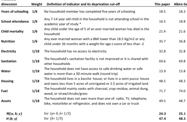
This section illustrates the ideas introduced in the preceding sections of the paper with an application to India using data from the Third National Family Health Survey (NFHS3) for 2005-6. In part, the motivation for using these data is that they have recently been used by Alkire and Seth (2009, 2013) for an analysis of multidimensional poverty in India following the AF methodology, and thus offer a useful point of comparison. The empirical
implementation thus closely follows Alkire-Seth definitions of dimensional indicators, cut-offs and weights (as set out in Table 4.1 in Alkire and Seth, 2013).34 In brief, Alkire-Seth use a
slightly modified version of the UNDP MPI methodology for India, under which there are 10 unequally-weighted indicators or dimensions, each represented by a binary variable
indicating the presence or absence of the particular deprivation for a person.35 Amongst the
10 indicators, there are two for education with weights of 1/6th each, two for health also with
weights of 1/6th each, and six indicators related to the standard of living each with a weight of
1/18th.36 The cross-dimensional cut-off is set at 1/3; thus, a person is deemed poor if
deprived in at least one-third of weighted dimensions. With this setup, multidimensional poverty measures 𝑀(𝛼, 𝛽; 𝑦) and 𝑀(𝛼, 𝑘; 𝑦) are constructed below for 𝑘 = 1/3 and different values of 𝛽. The illustration aims to highlight five points as noted in the Introduction. (i) A significant fraction of multidimensional poverty can be potentially missed by not counting deprivations of those below the cross-dimensional cut-off. Table 1 reports multidimensional poverty measures both in the aggregate as well as disaggregated by the breadth of dimensional deprivation. The estimates show that about 47% of the Indian population are deprived in one-third or more of the 10 weighed dimensions and are thus deemed to be poor under the dual cut-off approach. However, there is another 41% of the population who also experience deprivations, albeit in less than one-third of weighted dimensions. If these deprivations were to be counted in, multidimensional poverty would be
34 Estimates of the percentage of population deprived in each dimension and the corresponding AF
multidimensional poverty measures in this paper are close, though not identical, to those reported in Alkire and Seth (2013); see Table A1, Appendix 2 for a comparison. An exact replication is however not necessary for the purposes of this paper.
35 Since we are dealing with only binary variables, this is equivalent to 𝛼 = 0.
36 The NFHS3 data set can be used to construct observations on the 10 indicators for a
nationally-representative sample of 516,251 individuals in 108,938 households. Details on the sample design and methodology for NFHS3 can be found in IIPS and Macro International (2007). Further details on the dimensional indicators, weights and cut-offs can be found in Table A1, Appendix 2.