SFB 649 Discussion Paper 2008-045
Measuring and
Modeling Risk Using
High-Frequency Data
Wolfgang Härdle*
Nikolaus Hautsch*
Uta Pigorsch**
* Humboldt-Universität zu Berlin, Germany ** Universität Mannheim, Germany
This research was supported by the Deutsche
Forschungsgemeinschaft through the SFB 649 "Economic Risk". http://sfb649.wiwi.hu-berlin.de
ISSN 1860-5664
SFB 649, Humboldt-Universität zu Berlin Spandauer Straße 1, D-10178 Berlin
S
FB
6
4
9
E
C
O
N
O
M
I
C
R
I
S
K
B
E
R
L
I
N
High-Frequency Data
Wolfgang H¨ardle† Nikolaus Hautsch‡ Uta Pigorsch§ June 20, 2008
Abstract
Measuring and modeling financial volatility is the key to derivative pricing, asset allocation and risk management. The recent availabil-ity of high-frequency data allows for refined methods in this field. In particular, more precise measures for the daily or lower frequency volatility can be obtained by summing over squared high-frequency re-turns. In turn, this so–called realized volatility can be used for more accurate model evaluation and description of the dynamic and distri-butional structure of volatility. Moreover, non-parametric measures of systematic risk are attainable, that can straightforwardly be used to model the commonly observed time-variation in the betas. The discussion of these new measures and methods is accompanied by an empirical illustration using high-frequency data of the IBM incorpo-ration and of the DJIA index.
Keywords: Realized Volatility, Realized Betas, Volatility Modeling
JEL classification: C13, C14, C22, C52, C53
∗Financial support from the Deutsche Forschungsgemeinschaft through the SFB 649 “ ¨Okonomisches Risiko” is gratefully acknowledged.
†CASE - Center for Applied Statistics and Economics, School of Business and Economics, Humboldt-Universit¨at zu Berlin, Spandauerstr. 1, 10178 Berlin, Email:
‡Institute for Statistics and Econometrics, School of Business and Economics, Humboldt-Universit¨at zu Berlin, Spandauerstr. 1, D-10178 Berlin, Germany, Email:
§Department of Economics, University of Mannheim, L7,3-5, D-28131 Mannheim, Ger-many,Email: [email protected]
High-Frequency Data
Wolfgang H¨ardle, Nikolaus Hautsch and Uta Pigorsch
13.1 Introduction
Volatility modelling is the key to the theory and practice of pricing finan-cial products. Asset allocation and portfolio as well as risk management depend heavily on a correct modelling of the underlying(s). This insight has spurred extensive research in financial econometrics and mathematical finance. Stochastic volatility models with separate dynamic structure for the volatility process have been in the focus of the mathematical finance liter-ature, see Heston (1993) and Bates (2000), while parametric GARCH-type models for the returns of the underlying(s) have been intensively analyzed in financial econometrics.
The validity of these models in practice though depends upon specific dis-tributional properties or the knowledge of the exact (parametric) form of the volatility dynamics. Moreover, the evaluation of the predictive ability of volatility models is quite important in empirical applications. However, the latent character of the volatility poses a problem. To what measure should the volatility forecasts be compared to? Conventionally, the forecasts of daily volatility models, such as GARCH-type or stochastic volatility models, have been evaluated with respect to absolute or squared daily returns. In view of the excellent in-sample performance of these models, the forecasting perfor-mance, however, seems to be disappointing.
The availability of ultra-high-frequency data opens the door for a refined measurement of volatility and model evaluation. An often used and very flexible model for logarithmic prices of speculative assets is the (continuous-time) stochastic volatility model:
where σ2t is the instantaneous (spot) variance, µ denotes the drift, β is the risk premium, and Wt defines the standard Wiener process. The object of
interest is the amount of variation accumulated in a time interval ∆ (e.g., a day, week, month etc.). If n = 1,2, . . . denotes a counter for the time intervals of interest, then the term
σn2 =
Z n∆
(n−1)∆
σt2dt (13.2)
is called the actual volatility, see Barndorff-Nielsen and Shephard (2002). The actual volatility is the quantity that reflects the market risk structure (scaled in ∆) and is the key element in pricing and portfolio allocation. Actual volatility (measured in scale ∆) is of course related to the integrated volatility:
V(t) =
Z t
0
σs2ds. (13.3) It is worth noting that there is a small notational confusion here: the mathe-matical finance literature would denoteσt as “volatility” andσt2 as “variance”,
see Nelson and Foster (1994), for example.
An important result is that V(t) can be estimated from Yt via the quadratic
variation:
[Yt]M =
X
(Ytj −Ytj−1)
2, (13.4)
where t0 = 0 < t1 < · · · < tM = t is a sequence of partition points and
supj |tj+1 −tj| → 0. Andersen and Bollerslev (1998) have shown that
[Yt]M p
→V(t), M → ∞. (13.5) This observation leads us to consider in an interval ∆ with M observations
RVn = M X j=1 (Ytj −Ytj−1) 2 (13.6)
with tj = ∆{(n − 1) + j/M}. Note that RVn is a consistent estimator of
σ2n and is called realized volatility. Barndorff-Nielsen and Shephard (2002) point out that RVn −σn2 is approximately mixed Gaussian and provide the
asymptotic law of √
M(RVn −σn2). (13.7)
The realized volatility turns out to be very useful in the assessment of the validity of volatility models. For instance, reconciling evidence in favor of the forecast accuracy of GARCH-type models is observed when using realized
volatility as a benchmark rather than daily squared returns. Moreover, the availability of the realized volatility measure initiated the development of a new and quite accurate class of volatility models. In particular, based on the ex-post observability of the realized volatility measure, volatility is now treated as an observed rather than a latent variable to which standard time series procedures can be applied.
The remainder of this chapter is structured as follows. We first discuss the practical problems encountered in the empirical construction of realized volatility which are due to the existence of market microstructure noise. Sec-tion 13.3 presents the stylized facts of realized volatility, while SecSec-tion 13.4 reviews the most popular realized volatility models. Section 13.5 illustrates the usefulness of the realized volatility concept for measuring time-varying systematic risk within a conditional asset pricing model (CAPM).
13.2 Market Microstructure Effects
The consistency of the realized volatility estimator builds on the notion that prices are observed in continuous time and without measurement error. In practice, however, the sampling frequency is inevitably limited by the actual quotation or transaction frequency. Since high-frequency prices are subject to market microstructure noise, such as price-discreteness, bid-and-ask bounce effects, transaction costs etc., the true price is unobservable. Market mi-crostructure effects induce a bias in the realized volatility measure, which can straightforwardly be illustrated in the following simple discrete-time setup. Assume that the logarithmic high-frequency prices are observed with noise, i.e.,
Ytj = Y ∗
tj + εtj, (13.8)
where Yt∗j denotes the latent true price. Moreover, the microstructure noise
εtj is assumed to be iid distributed with mean zero and variance η
2, and is
independent of the true return. Let r∗tj denote the efficient return, then the high-frequency continuously compounded returns
rtj = r ∗
tj + εtj −εtj−1 (13.9)
follow an MA(1) process. Such a return specification is well established in the market microstructure literature and is usually justified by the existence of the bid-ask bounce effect, see, e.g., Roll (1984). In this model, the realized
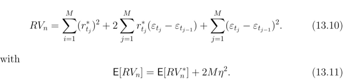
volatility is given by RVn = M X i=1 (r∗tj)2 + 2 M X j=1 rt∗j(εtj −εtj−1) + M X j=1 (εtj −εtj−1) 2 . (13.10) with E[RVn] = E[RVn∗] + 2M η 2. (13.11)
If the sampling frequency goes to infinity, we know from the previous section thatRVn∗ consistently estimatesσn2 and, thus, the realized volatility based on the observed price process is a biased estimator of the actual volatility with bias term 2M η2. Obviously, for M → ∞, RVn diverges.
1 5 10 50 100 500 1000
3200
3600
4000
4400
sampling frequency in ticks
RV
Figure 13.1. Volatility signature plot for IBM, 2001-2006. Average time between trades: 6.78 seconds. XFGsignature
This diverging behavior can also be observed empirically in so–called volatil-ity signature plots. Figure 13.1 shows the volatilvolatil-ity signature for one stock of the IBM incorporation over the period ranging from January 2, 2001 to December 29, 2006. The plot depicts the average annualized realized volatil-ity over the full sample period constructed at different frequencies measured in number of ticks (depicted in log scale). Obviously, the realized volatility is large at the very high frequency, but decays for lower frequencies and sta-bilizes around a sampling frequency of 300 ticks, which corresponds approx-imately to a 30 minute sampling frequency, given that the average duration between two consecutive trades is around 6.78 seconds.
Thus, sampling at a lower frequency, such as every 10, 15 or 30 minutes, seems to alleviate the problem of market microstructure noise and has thus
frequently been applied in the literature. This so–called sparse sampling, however, comes at the cost of a less precise estimate of the actual volatility. Alternative methods have been proposed to solve this bias-variance trade-off for the above simple noise assumption as well as for more general noise pro-cesses, allowing also for serial dependence in the noise and/or for dependence between the noise and the true price process, which is sometimes referred to as endogenous noise. A natural approach to reduce the market microstructure noise effect is to construct the realized volatility measure based on prefiltered high-frequency returns, using, e.g., an MA(1) model.
In the following we briefly present two more elaborate and under specific noise assumptions consistent procedures for estimating actual volatility. Both have been theoretically considered in several papers. The subsampling approach originally suggested by Zhang et al. (2005) builds on the idea of averaging over various realized volatilities constructed from different high-frequency subsamples. For the ease of exposition we focus again on one time period, e.g., one day, and denote the full grid of time points at which theM intradaily prices are observed by Gt = {t0, . . . , tM}. The realized volatility that makes
use of all observations in the full grid is denoted byRVn(all). Moreover, the grid
is partitioned intoL nonoverlapping subgridsG(l),l = 1, . . . , L. A simple way
for selecting such a subgrid may be the so–called regular allocation, in which the l-th subgrid is given by G(l) = {t
l−1, tl−1+L, . . . , tl−1+MlL} for l = 1, . . . , L,
and Ml denoting the number of observations in each subgrid. E.g., consider
5-minute returns that can be measured at the time points 9:30, 9:35, 9:40,
. . ., and at the time points 9:31, 9:36, 9:41,. . . and so forth. In analogy to the full grid, the realized volatility for subgridl, denoted by RVn(l), is constructed
from all data points in subgrid l. Thus, RVn(l) is based on sparsely sampled
data.
The actual volatility is then estimated by:
RVn(ZM A) = 1 L L X l=1 RVn(l)− M¯ MRV (all) n , (13.12) where ¯M = L1 PL
l=1Ml. The latter term on the right-hand side is included to
bias-correct the averaging estimator L1 PL
l=1RV (l)
n . As the estimator (13.12)
consists of a component based on sparsely sampled data and one based on the full grid of price observations, the estimator is also called the two time scales estimator.
Given the similarity to the problem of estimating the long-run variance of a stationary time series in the presence of autocorrelation, it is not surprising that kernel-based methods have been developed for estimating the realized
volatility. Most recently, Barndorff-Nielsen et al. (2008) proposed the flat-top realized kernel estimator
RVn(BHLS) = RVn+ H∗ X h=1 K h−1 H∗ (bγh+bγ−h) (13.13) with b γh = M M −h M X j=1 rtjrtj−h, (13.14)
and K(0) = 1, K(1) = 0. Obviously, the summation term on the right-hand side is the realized kernel correction of the market microstructure noise. Zhou (1996), who was the first to consider realized kernels, proposed (13.13) with H = 1, while Hansen and Lunde (2006) allowed for general H but restricted K(x) = 1. Both of these estimators, however, have been shown to be inconsistent. Barndorff-Nielsen et al. (2008) instead propose several consistent realized kernel estimators with an optimally chosen H∗, such as the Tukey-Hanning kernel, i.e. K(x) = {1−cosπ(1−x)2}/2, which performs also very well in terms of efficiency as illustrated in a Monte Carlo analysis. They further show, that these realized kernel estimators are robust to market microstructure frictions that may induce endogenous and dependent noise terms.
13.3 Stylized Facts of Realized Volatility
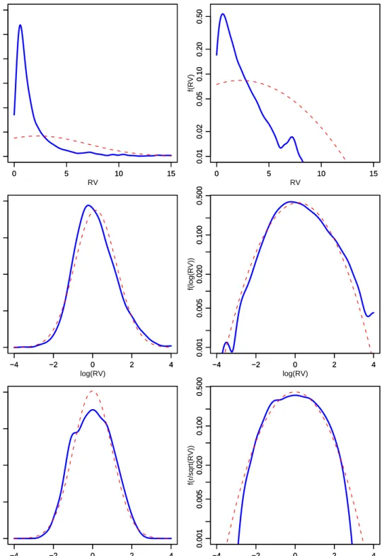
Figure 13.2 shows kernel density estimates of the plain and logarithmic daily realized volatility in comparison to plots of a correspondingly fitted (log) normal distribution based on the IBM data, 2001-2006. The pictures in the top of Figure 13.2 show the unconditional distribution of the (plain) realized volatility in contrast to a fitted normal distribution. As also confirmed by the corresponding descriptive statistics displayed by Table 13.1, we observe that realized volatility reveals severe right-skewness and excess kurtosis. This re-sult might be surprising given that the realized volatility consists of the sum of squared intra-day returns and thus central limit theorems should apply. However, it is a common finding that intra-day returns are strongly serially dependent requiring significantly higher intra-day sampling frequencies to ob-serve convergence to normality. In contrast, the unconditional distribution of the logarithmic realized volatility is well approximated by a normal distribu-tion. The sample kurtosis is strongly reduced and is close to 3. Though slight right-skewness and deviations from normality in the tails of the distribution
0 5 10 15 0.0 0.1 0.2 0.3 0.4 0.5 0.6 RV f(RV) 0 5 10 15 0.0 0.1 0.2 0.3 0.4 0.5 0.6 0 5 10 15 0.01 0.02 0.05 0.10 0.20 0.50 RV f(RV) 0 5 10 15 0.01 0.02 0.05 0.10 0.20 0.50 −4 −2 0 2 4 0.0 0.1 0.2 0.3 0.4 log(RV) f(log(RV)) −4 −2 0 2 4 0.0 0.1 0.2 0.3 0.4 −4 −2 0 2 4 0.001 0.005 0.020 0.100 0.500 log(RV) f(log(RV)) −4 −2 0 2 4 0.001 0.005 0.020 0.100 0.500 −4 −2 0 2 4 0.0 0.1 0.2 0.3 0.4 r/sqrt(RV) f(r/sqrt(RV)) −4 −2 0 2 4 0.0 0.1 0.2 0.3 0.4 −4 −2 0 2 4 0.001 0.005 0.020 0.100 0.500 r/sqrt(RV) f(r/sqrt(RV)) −4 −2 0 2 4 0.001 0.005 0.020 0.100 0.500
Figure 13.2. Kernel density estimates of the (logarithmic) re-alized volatility and of correspondingly standardized returns for IBM, 2001-2006. The dotted line depicts the density of the correspondingly fitted normal distribution. The left column depicts the kernel density estimates based on a log scale. XFGkernelcom
are still observed, the underlying distribution is remarkably close to that of a Gaussian distribution.
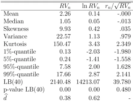
RVn lnRVn rn/ √ RVn Mean 2.26 0.14 -.000 Median 1.05 0.05 -.013 Skewness 9.93 0.42 .035 Variance 22.57 1.13 .979 Kurtosis 150.47 3.43 2.349 1%-quantile 0.13 -2.03 -1.980 5%-quantile 0.24 -1.41 -1.558 95%-quantile 7.58 2.00 1.628 99%-quantile 17.66 2.87 2.141 LB(40) 2140.48 14213.07 39.780 p-value LB(40) 0.00 0.00 0.480 b d 0.38 0.62
-Table 13.1. Descriptive statistics of the realized volatility, log realized volatility and standardized returns, IBM stock, 2001-2006. LB (40) denotes the Ljung-Box statistic based on 40 lags. The last row gives an estimate of the order of fractional integration based on the Geweke and Porter-Hudak estimator.
XFGIBm
A common finding is that financial returns have fatter tails than the normal distribution and reveal significant excess kurtosis. Though GARCH models can explain excess kurtosis, they cannot completely capture these properties in real data. Consequently, (daily) returns standardized by GARCH-induced volatility, typically still show clear deviations from normality. However, a striking result in recent literature is that return series standardized by the square root of realized volatility, rn/
√
RVn, are quite close to normality. This
result is illustrated by the plots in the bottom of Figure 13.2 and the descrip-tive statistics in Table 13.1. Though we observe deviations from normality for returns close to zero resulting in a kurtosis which is even below 3, the fit in the tails of the distribution is significantly better than that for plain log returns. Summarizing the empirical findings from Figure 13.2, we can con-clude that the unconditional distribution of daily returns is well described by a lognormal-normal mixture. This confirms the mixture-of-distribution hypothesis by Clark (1973) as well as the idea of the basic stochastic volatil-ity model, where the log variance is modelled in terms of a Gaussian AR(1) process.
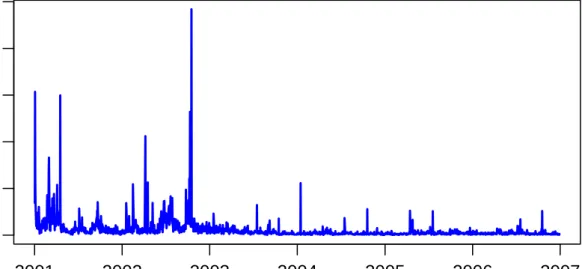
Figure 13.3 shows the evolvement of daily realized volatility over the analyzed sample period and the implied sample autocorrelation functions (ACFs). As also shown by the corresponding Ljung-Box statistics in Table 13.1, the re-alized volatility is strongly positively autocorrelated with high persistence. This is particularly true for the logarithmic realized volatility. The plot
0 20 40 60 80 100 time RV 2001 2002 2003 2004 2005 2006 2007 0 20 40 60 80 100 120 0.0 0.2 0.4 0.6 0.8 1.0 lag ACF 0 20 40 60 80 100 120 0.0 0.2 0.4 0.6 0.8 1.0 lag ACF
Figure 13.3. Time evolvement and sample autocorrela-tion funcautocorrela-tion of the realized volatility for IBM, 2001-2006.
XFGrvtsacf
shows that the ACF decays relatively slowly providing hints on the existence of long range dependence. Indeed, a common finding is that the realized volatility processes reveal long range dependence which is well captured by fractionally integrated processes. In particular, if RVn is integrated of the
order d ∈ (0,0.5), it can be shown that
Var " h X j=1 RVn+j # ≈ ch2d+1, (13.15)
with c denoting a constant. Then, plotting lnVarhPh
j=1RVn+j
i
against lnh
strongly confirm this relationship and find values for d between 0.35 and 0.4 providing clear evidence for long range dependence. Estimating d using the Geweke and Porter-Hudak estimator, we obtain db= 0.38 for the series of
realized volatilities and db= 0.62 for its logarithmic counterpart. Hence, for
both series we find clear evidence for long range dependence. However, the persistence in logarithmic realized volatilities is remarkably high providing even hints on non-stationarity of the process.
Summarizing the most important empirical findings, we can conclude that the unconditional distributions of logarithmic realized volatility and of cor-respondingly standardized log returns are well approximated by normal dis-tributions and that realized volatility itself follows a long memory process. These results suggest (Gaussian) ARFIMA models as valuable tools to model and to predict (log) realized volatility.
13.4 Realized Volatility Models
As illustrated above, realized volatility models should be able to capture the strong persistence in the sample autocorrelation function. While this seemingly long-memory pattern is widely acknowledged, there is still no con-sensus on the mechanism generating it. One approach is to assume that the long memory is generated by a fractionally integrated process as origi-nally introduced by Granger and Joyeux (1980) and Hosking (1981). In the GARCH literature this has lead to the development of the fractionally inte-grated GARCH model as, e.g., proposed by Baillie et al. (1996). For realized volatility the use of a fractionally integrated autoregressive moving average (ARFIMA) process was advocated, for example, by Andersen et al. (2003). The ARFIMA(p, q) model is given by
φ(L)(1−L)d(yn −µ) = ψ(L)un, (13.16)
with φ(L) = 1−φ1L−. . .−φpLp, ψ(L) = 1 +ψ1L+. . . ψqLq, and d denoting
the fractional difference parameter. Moreover, un is usually assumed to be a
Gaussian white noise process, andyn denotes either the realized volatility (see
Koopman et al. (2005)) or its logarithmic transformation. Several extensions of the realized volatility ARFIMA model have been proposed, accounting, for example, for leverage effects (see Martens et al. (2004)), for non–Gaussianity of (log) realized volatility or for time-variation in the volatility of realized volatility (see Corsi et al. (2008)). Generally the empirical results show sig-nificant improvements in the point forecasts of volatility when using ARFIMA rather than GARCH-type models.
An alternative model for realized volatility has been suggested by Corsi (2004). The so-called heterogeneous autoregressive (HAR) model of realized volatility approximates the long-memory pattern by a sum of multi-period volatility components. The simulation results in Corsi (2004) show, that the HAR model can quite adequately reproduce the hyperbolic decay in the sample autocorrelation function of realized volatility even if the number of volatility components is small. For the HAR model, let the k–period realized volatility component be defined by the average of the single-period realized volatilities, i.e., RVn+1−k:n = 1 k k X j=1 RVn−j. (13.17)
The HAR model with the so-defined daily, weekly and monthly realized-volatility components, is given by
logRVn = α0 +αdlogRVn−1 +αwlogRVn−5:n−1
+αmlogRVn−21:n−1 +un, (13.18)
with un typically being a Gaussian white noise. The HAR model has become
very popular due to its simplicity in estimation and its excellent in-sample fit and predictive ability (see e.g. Andersen et al. (2004), Corsi et al. (2008)). Several extensions exist and deal, for example, with the inclusion of jump measures (see Andersen et al. (2004)) or non-linear specifications based on neural networks (see Hillebrand and Medeiros (2007)).
Alternative realized volatility models have been proposed in, e.g., Barndorff-Nielsen and Shephard (2002), who consider a superposition of Ornstein– Uhlenbeck processes, and in Deo et al. (2006), who specify a long-memory stochastic volatility model. A recent and comprehensive review on realized volatility models can also be found in McAleer and Medeiros (2008).
13.5 Time-Varying Betas
So far, our discussion focused on the measurement and modeling of the volatil-ity of a financial asset using high-frequency transaction data. From a pricing perspective, however, systematic risk is most important. In this section, we therefore discuss, how high-frequency information can be used for the evalua-tion and modeling of systematic risk. A common measure for the systematic risk is given by the so-called (market) beta, which represents the sensitivity of a financial asset to movements of the overall market. As the beta plays a
crucial role in asset pricing, investment decisions, and the evaluation of the performance of asset managers, a precise estimate and forecast of betas is indispensable. While the unconditional capital asset pricing model implies a linear and stable relationship between the asset’s return and the system-atic risk factor, i.e., the return of the market, empirical results suggest that the beta is time-varying, see, for example, Bos and Newbold (1984), Hafner and Herwartz (1973), and Fabozzi and Francis (1978). Similar evidence has been found for multi-factor asset pricing models, where the factor loadings seem to be time-varying rather than constant. A large amount of research has therefore been devoted to conditional CAPM and APT models, which allow for time-varying factor loadings, see, for example, Dumas and Solnik (1995), Ferson and Harvey (1991), Ferson and Harvey (1993), and Ferson and Korajcyzyk (1995).
13.5.1 The Conditional CAPM
Below we consider the general form of the conditional CAPM. A similar dis-cussion for multi-factor models can be found in Bollerslev and Zhang (2003). Assume that the continuously compounded return of a financial asset i from period n to n+ 1 is generated by the following process
ri;n+1 = αi;n+1|n+βi;n+1|nrm;n+1 +ui;n+1, (13.19)
with rm;n+1 denoting the excess market return and αn+1|n denoting the
inter-cept that may be time-varying conditional on the information set available at time n, as indicated by the subscript. The idiosyncratic risk un+1 is serially
uncorrelated, En(un+1) = 0, but may exhibit conditionally time-varying
vari-ance. Note that En(·) denotes the expectation conditional on the information
set available at time n. Moreover, we assume that E(rm;n+1un+1) = 0 for all
n. The conditional beta coefficient of the CAPM regression (13.19) is defined as
βi;n+1|n = Cov(ri;n+1, rm;n+1)
Var(ri;n+1)
. (13.20)
Now, assume that lending and borrowing at a one-period risk-free rate rf;n
is possible. Then, the arbitrage-pricing theory implies that the conditional expectation of the next period’s return at time n is given by
En(ri;n+1) = rf;n +βi;n+1|nEn(rm;n+1). (13.21)
Thus, the computation of the future return of asset i requires to specify how the beta coefficient evolves over time.
The most common approach to allow for time-varying betas is to re-run the CAPM regression in each period based on a sample of 3 or 5 years. We refer to this as the rolling regression (RR) method. More elaborate estimates of the beta can be obtained using the Kalman-filter, which builds on a state-space representation of the conditional CAPM or by specifying a dynamic model for the covariance matrix between the return of asset i and the market return.
13.5.2 Realized Betas
The evaluation of the in-sample fit and predictive ability of various beta mod-els is also complicated by the unobservability of the true beta. Consequently, model comparisons are usually conducted in terms of implied pricing errors, i.e., ei,n+1 = rbi,n+1 − ri,n+1, with bri,n+1 = rf;n + βbi;n+1|nEn(rm;n+1). Owing
to the discussion on the evaluation of volatility models, the question arises, whether high-frequency data may also be useful for the evaluation of com-peting beta estimates. The answer is a clear “yes”. In fact, high-frequency based estimates of betas are quite informative for the dynamic behavior of systematic risk. The construction of so-calledrealized betas is straightforward and builds on realized covariance and realized volatility measures. In partic-ular, denote the realized volatility of the market by RVm;n and the realized
covariance between the market and asset i by RCovm,i;n =
PM
j=1ri,tjrm,tj,
where ri,tj and rm,tj denote the j-th high-frequency return of the asset and
the market, respectively, during day n. The realized beta is then defined as
b
βHF;i;n =
RCovm,i;n
RVm;n
. (13.22)
Barndorff-Nielsen and Shephard (2004) show that the realized beta converges almost surely for allnto the integrated beta over the time period fromn−1 to
n, i.e., the daily systematic risk associated with the market index. Note that the realized beta can also be obtained from a simple regression of the high-frequency returns of asset i on the high-frequency returns of the market, see, e.g., Andersen et al. (2006). The preciseness of the realized beta estimator can easily be assessed by constructing the (1−α)-percent confidence intervals, which have been derived in Barndorff-Nielsen and Shephard (2004) and are given by b βHF;i;n±zα/2 v u u u t M X j=1 r2m,tj !−2 b gi;n, (13.23)
where zα/2 denotes the (α/2)-quantile of the standard normal distribution, b gi;n = M X j=1 x2i;j − M−1 X j=1 xi;jxi;j+1, (13.24) and xi;j = ri,tjrm,tj −βbHF;i;nr 2 m,tj. (13.25)
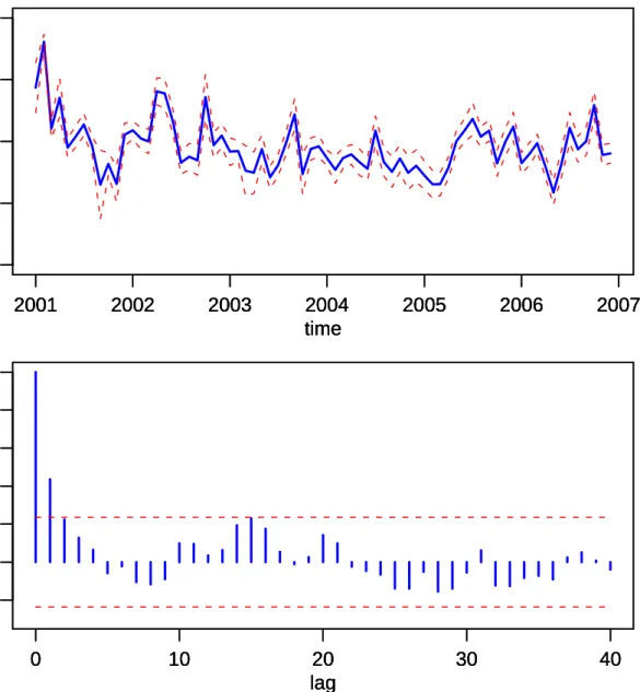
The upper panel in Figure 13.4 presents the time-evolvement of the monthly
0.0 0.5 1.0 1.5 2.0 time beta 2001 2002 2003 2004 2005 2006 2007 0.0 0.5 1.0 1.5 2.0 time beta 2001 2002 2003 2004 2005 2006 2007 0.0 0.5 1.0 1.5 2.0 time beta 2001 2002 2003 2004 2005 2006 2007 0 10 20 30 40 −0.2 0.2 0.6 1.0 lag ACF 0 10 20 30 40 −0.2 0.2 0.6 1.0 lag ACF 0 10 20 30 40 −0.2 0.2 0.6 1.0 lag ACF
Figure 13.4. Time evolvement and sample autocorrelation function of monthly realized betas for IBM, 2001-2006. The dashed lines in the upper panel present the 95% confidence intervals of the realized beta estimator as given in (13.23). The dashed lines in the lower panel depict the 95% Bartlett confidence intervals. XFGbetatsacf
realized beta for IBM incorporation over the period ranging from 2001 to 2006. We use the Dow Jones Industrial Average Index as the market in-dex and construct the realized betas using 30 minute returns. The graph also shows the 95%-confidence intervals of the realized beta estimator. The time-varying nature of systematic risk emerges strikingly from the figure and provides once more evidence for the relevance of its inclusion in asset pricing models.
Interestingly, the sample autocorrelation function of the realized betas de-picted in the lower panel of Figure 13.4 indicates significant serial correlation over the short horizon. This dependency can be explored for the prediction of systematic risk. Bollerslev and Zhang (2003), for example, find that an au-toregressive model for the realized betas outperforms the RR approach both in terms of forecast accuracy as well as in terms of pricing errors.
13.6 Summary
We review the usefulness of high-frequency data for measuring and modeling actual volatility at a lower frequency, such as a day. We present the realized volatility as an estimator of the actual volatility along with the practical prob-lems arising in the implementation of this estimator. We show that market microstructure effects induce a bias to the realized volatility and we discuss several approaches for the alleviation of this problem. The realized volatility is a more precise estimator of the actual volatility than the conventionally used daily squared returns, and thus provides more accurate information on the distributional and dynamic properties of volatility. This is important for many financial applications, such as asset pricing, portfolio allocation or risk management. As a consequence, several modeling approaches for real-ized volatility exist and have been shown to usually outperform traditional GARCH or stochastic volatility models, both in terms of in-sample as well as out-of-sample performance. We further demonstrate the usefulness of the realized variance and covariance estimator for measuring and modeling sys-tematic risk. For the empirical examples provided in this chapter we use tick-by-tick transaction data of one stock of the IBM incorporation and of the DJIA index.
Bibliography
P. R. Hansen and A. Lunde (2006). Realized Variance and Market Microstructure Noise,
Journal of Business & Economic Statistics 24: 127-161.
B. Zhou (1996). High-Frequency Data and Volatility in Foreign-Exchange Rates,Journal of Business & Economic Statistics 14: 45-52.
Ole E. Barndorff-Nielsen, Peter R. Hansen, Asger Lunde and Neil Shephard (2008). Design-ing Realised Kernels to Measure the ex-post Variation of Equity Prices in the Presence of Noise, Econometrica, forthcoming.
L. Zhang, P. A. Mykland and Y. Ait-Sahalia(1005). A Tale of Two Time Scales:
Determin-ing Integrated Volatility With Noisy High-Frequency Data, Journal of the American
Statistical Association 100(472): 1394-1411.
R. Roll (1984). A Simple Implicit Measure of the Effective Bid-Ask Spread in an Efficient Market, Journal of Finance 39: 1127-1139.
O. E. Barndorff-Nielsen and N. Shephard (2002). Estimating Quadratic Variation Using Realized Variance, Journal of Applied Econometrics4,5: 457-477.
D. S. Bates (2000). Post-’87 Crash Fears in the S&P 500 Futures Option,Journal of Econo-metrics 94,1-2: 181-238.
S. L. Heston, (1993). A Closed-Form Solution for Options with Stochastic Volatility with
Applications to Bond and Currency Options, The Review of Financial Studies 6(2):
327-343.
T. G. Andersen and T. Bollerslev, (1997). Heterogeneous Information Arrivals and
Re-turn Volatility Dynamics: Uncovering the Long-Run in High Frequency ReRe-turns, The
Journal of Finance 52: 975-1005.
T. G. Andersen, T. Bollerslev, F. X. Diebold and P. Labys (2001). The Distribution of Real-ized Exchange Rate Volatility, Journal of the American Statistical Association 96: 42-55.
T. G. Andersen, T. Bollerslev, F. X. Diebold and P. Labys (2003). Modeling and Forecasting Realized Volatility, Econometrica 71: 579-625.
T. G. Andersen, T. Bollerslev, F. X. Diebold and J. Wu, (2006). Realized Beta: Persistence and Predictability, Advances in Econometrics: Econometric Analysis of Economic and Financial Time Series, Volume B Editor: T.Fomby: 1-40.
T. G. Andersen and T. Bollerslev (1998). Answering the Skeptics: Yes, Standard Volatility Models do Provide Accurate Forecasts, International Economic Review39: 885-905. T. G. Andersen, T. Bollerslev and F. X. Diebold, (2008). Roughing it Up: Including Jump
Components in the Measurement, Modeling and Forecasting of Return Volatility,
Re-view of Economics and Statistics, forthcoming.
Torben G. Andersen, Tim Bollerslev and Xin Huang (2006). A Semiparametric Frame-work for Modeling and Forecasting Jumps and Volatility in Speculative Prices, Duke University, Working Paper.
R. T. Baillie, T. Bollerslev and H. O. Mikkelsen (1996). Fractionally Integrated Generalized Autoregressive Conditional Heteroskedasticity, Journal of Econometrics 74: 3-30. F. M. Bandi, J. R. Russell and J. Zhu (2008). Using High-Frequency Data in Dynamic
O. E. Barndorff-Nielsen and N. Shephard(2002). Econometric Analysis of Realised Volatility and its Use in Estimating Stochastic Volatility Models,Journal of the Royal Statistical Society, Series B64: 253-280.
O. E. Barndorff-Nielsen and N.S hephard (2004). Econometric Analysis of Realized Co-variation: High Frequency Based Covariance, Regression, and Correlation in Financial Economics, Econometrica 72: 885-925.
G. H. Bauer and K. Vorkink (2007 ). Multivariate Realized Stock Market Volatility, Bank of Canada, Working Paper.
T. Bollerslev, U. Kretschmer, C. Pigorsch, and G. Tauchen(2008). A Discrete-Time Model for Daily S&P500 Returns and Realized Variations: Jumps and Leverage Effects, Journal of Econometrics, forthcoming.
M. Blume (1975). Betas and Their Regression Tendencies,Journal of Finance 30: 785-95. T. Bollerslev, R. F. Engle, J. M. Wooldridge (1988). A Capital Asset Pricing Model with
Time Varying Covariances, Journal of Political Economy96: 116-131.
T. Bollerslev and B. Y. B. Zhang (2003). Measuring and Modeling Systematic Risk in Factor Pricing Models Using High-frequency Data,Journal of Empirical Finance 10: 533-558. T. Bos and P. Newbold(1984). An Empirical Investigation of the Possibility of Stochastic
Systematic Risk in the Market Model,Journal of Business 57: 35-41.
P. A. Braun, D. B. Nelson and A. M. Sunier (1995). Good News, Bad News, Volatility, and Betas,Journal of Business 50: 1575-1603.
R. Chiriac and V. Voev (2007). Long Memory Modelling of Realized Covariance Matrices,
University of Konstanz, Working Paper.
F. Corsi, S. Mittnik, C. Pigorsch and U. Pigrosch (2008). The Volatility of Realized Volatility,
Econometric Reviews27: 46-78.
D. W. Collins, J. Ledolter and J. Rayburn (1987). Some Further Evidence on the Stochastic Properties of Systematic Risk,Journal of Business 60: 425-448.
F.Corsi (2004). A Simple Long Memory Model of Realized Volatility,University of Southern Switzerland, Woking Paper.
Z. Da and E. Schaumburg (2006). The Factor Structure of Realized Volatility and its Im-plications for Option Pricing, University of Notre Dame, Working Paper.
R. Deo, C. Hurvich and Y. Lu (2006). Forecasting Realized Volatility Using a Long-Memory Stochastic Volatility Model: Estimation, Prediction and Seasonal Adjustment,Journal of Econometrics131(1-2): 29-58.
F. X. Diebold and A. Inoue (2001). Long Memory and Regime Switching , Journal of
Econometrics 2001: 131-159.
B. Dumas and B. Solnik (1995). The World Price of Exchange Rate Risk,Journal of Finance 50: 445-480.
R. F. Engle and G. G. J. Lee (1999). A Permanent and Transitory Component Model of Stock Return Volatility, Cointegration, Causality, and Forecasting: A Festschrift in Honor of Clive W. J. Granger: 475-497.
F. J. Fabozzi and J. C. Francis (1978). Beta as a Random Coefficient, Journal of Financial and Quantitative Analysis13: 101-116.
R. W. Faff, D.Hillier and J. Hillier, (2000). Time Varying Beta Risk: An Analysis of Alter-native Modelling Techniques,Journal of Business, Finance and Accounting27: 523-554
W. E. Ferson and C. R. Harvey (1991). The Variation of Economic Risk Premiums,Journal of Poltical Economy 99: 385-415.
W. E. Ferson and C. R. Harvey (1993). The Risk and Predictability of International Equity Returns, Review of Financial Studies 6527-566.
W. E. Ferson and R. A. Korajczyk (1995). Do Arbitrage Pricing Models Explain the Pre-dictability of Stock Returns?, Journal of Business 68: 309-349.
C. Gourieroux and J. Jasiak (2001). Financial Econometrics: Problems, Models, and Meth-ods, Princeton University Press, Princeton
C. W. J. Granger (1980). Long Memory Relationships and the Aggregation of Dynamic Models, Journal of Econometrics 14: 227-238.
C. W. J. Granger and N. Hyung (2004). Occasional Structural Breaks and Long Memory with an Application to the S&P 500 Absolute Stock Returns, Journal of Empirical Finance 11: 399-421.
C. W. J. Granger and R. Joyeux (1980). An Introduction to Long-Range Time Series Models and Fractional Differencing, Journal of Time Series Analysis 1: 15-30.
C. W. J. Granger and T. Ter¨asvirta (1999). A Simple Nonlinear Time Series Model with
Misleading Linear Properties, Economic Letters 62: 161-165.
E. Hillebrand and M. Medeiros (2007). Forecasting Realized Volatility Models: the Benefits of Bagging and Non-Linear Specifications, Louisana State University, Working Paper. J. R. M. Hosking (1981). Fractional Differencing,Biometrika 68: 165-176.
N. L. Jacob (1971). The Measurement of Systematic Risk for Securities and Portfolios: Some Empirical Results, Journal of Financial and Quantitative Analysis 6: 815-834.
S. J. Koopman, B. Jungbacker and E. Hall.(2005). Forecasting Daily Variability of the S&P 100 Stock Index Using Historical, Realised and Implied Volatility Measurements,
Journal of Empirical Finance 12,3: 445-475.
X. Li (2003). On Unstable Beta Risk and Its Modelling Techniques for New Zealand Industry Portfolios, Massey University, Working Paper.
T. Lux and M. Marchesi (1999). Scaling and Criticality in a Stochastic Multi-Agent Model of a Financial Market, Nature397: 498-500
M. Martens, D. van Dijk and M.dePooter (2004). Modeling and Forecasting S&P 500 Volatil-ity: Long Memory, Structural Breaks and Nonlinearity, Erasmus University Rotterdam, Working Paper.
M. Martens and J. Zein (2004). Predicting Financial Volatility: High-Frequency Time-Series Forecasts vis-`a-vis Implied Volatility, Journal of Futures Markets 11: 1005-1028.
M. McAleer and M.Medeiros (2008). Realized Volatilty: A Review, Econometric Reviews
26: 10-45.
M. McAleer and M.Medeiros (2006). A Multiple Regime Smooth Transition Heterogenous
Autoregressive Model for Long Memory and Asymmetries, Pontifical Catholic
Univer-sity of Rio de Janeiro, Working Paper.
U. A. M¨uller, M. M. Dacorogna, R. D. Dav, R. B. Olsen, O. V. Pictet and J. E. von
Weizs¨acker(1997). Volatilities of Different Time Resolutions - Analyzing the Dynamics of Market Components, Journal of Empirical Finance 4(2-3); 213-239.
T. Mikosch and C. St˘aric˘a (2004). Nonstationarities in Financial Time Series, the
Long-range Dependence, and the IGARCH Effects, The Review of Economics and Statistics
D. B. Nelson and D. P. Foster (1994). Asymptotic Filtering Theory for Univariate ARCH Models,Econometrica 62: 1-41.
M. dePooter, M. Martens and D. van Dijk (). Predicting the Daily Covariance Matrix for
S&P 100 Stocks Using Intraday Data - But Which Frequency to Use?, Econoemtric
Reviews, forthcoming.
S. Pong, M. B. Shackleton, S. J. Taylor and X. Xu (). Forecasting Currency Volatility: A Comparison of Implied Volatilities and AR(FI)MA Models, Journal of Banking & Finance28: 2541-2563.
M. Scharth and M. Medeiros (2006). Asymmetric Effects and Long Memory in the Volatility of DJIA Stocks,Pontifical Catholic University of Rio de Janeiro, Working Paper. S. Sunder (1980). Stationarity of Market Risk: Random Coefficients Tests for Individual
Stocks, Journal of Finance 35: 883-896.
D. D. Thomakos (2003). Realized Volatility in the Futures Markets, Journal of Empirical Finance10: 321-353.
V. Voev (2008). Dynamic Modelling of Large-Dimensional Covariance Matrices, in High Frequency Financial Econometrics, edited by L.Bauwens, W.Pohlmeier and D.Veredas, Physica-Verlag, Heidelberg: 293-312.
C. M. Hafner and H. Herwartz (1998). Time Varying Market Price of Risk in the CAPM-Approaches, Empirical Evidence and Implications,Finance 19: 93-112.
P. K. Clark (1973). A Subordinated Stochastic Process Model with Finite Variance for Speculative Prices, Econometrica 41: 135-156.
For a complete list of Discussion Papers published by the SFB 649, please visit http://sfb649.wiwi.hu-berlin.de.
001 "Testing Monotonicity of Pricing Kernels" by Yuri Golubev, Wolfgang Härdle and Roman Timonfeev, January 2008.
002 "Adaptive pointwise estimation in time-inhomogeneous time-series models" by Pavel Cizek, Wolfgang Härdle and Vladimir Spokoiny,
January 2008.
003 "The Bayesian Additive Classification Tree Applied to Credit Risk Modelling" by Junni L. Zhang and Wolfgang Härdle, January 2008.
004 "Independent Component Analysis Via Copula Techniques" by Ray-Bing Chen, Meihui Guo, Wolfgang Härdle and Shih-Feng Huang, January 2008.
005 "The Default Risk of Firms Examined with Smooth Support Vector Machines" by Wolfgang Härdle, Yuh-Jye Lee, Dorothea Schäfer and Yi-Ren Yeh, January 2008.
006 "Value-at-Risk and Expected Shortfall when there is long range dependence" by Wolfgang Härdle and Julius Mungo, Januray 2008. 007 "A Consistent Nonparametric Test for Causality in Quantile" by
Kiho Jeong and Wolfgang Härdle, January 2008.
008 "Do Legal Standards Affect Ethical Concerns of Consumers?" by Dirk Engelmann and Dorothea Kübler, January 2008.
009 "Recursive Portfolio Selection with Decision Trees" by Anton Andriyashin, Wolfgang Härdle and Roman Timofeev, January 2008.
010 "Do Public Banks have a Competitive Advantage?" by Astrid Matthey,
January 2008.
011 "Don’t aim too high: the potential costs of high aspirations" by Astrid Matthey and Nadja Dwenger, January 2008.
012 "Visualizing exploratory factor analysis models" by Sigbert Klinke and Cornelia Wagner, January 2008.
013 "House Prices and Replacement Cost: A Micro-Level Analysis" by Rainer Schulz and Axel Werwatz, January 2008.
014 "Support Vector Regression Based GARCH Model with Application to Forecasting Volatility of Financial Returns" by Shiyi Chen, Kiho Jeong and Wolfgang Härdle, January 2008.
015 "Structural Constant Conditional Correlation" by Enzo Weber, January 2008.
016 "Estimating Investment Equations in Imperfect Capital Markets" by Silke Hüttel, Oliver Mußhoff, Martin Odening and Nataliya Zinych, January 2008.
017 "Adaptive Forecasting of the EURIBOR Swap Term Structure" by Oliver Blaskowitz and Helmut Herwatz, January 2008.
018 "Solving, Estimating and Selecting Nonlinear Dynamic Models without the Curse of Dimensionality" by Viktor Winschel and Markus Krätzig,
February 2008.
019 "The Accuracy of Long-term Real Estate Valuations" by Rainer Schulz, Markus Staiber, Martin Wersing and Axel Werwatz, February 2008. 020 "The Impact of International Outsourcing on Labour Market Dynamics in
Germany" by Ronald Bachmann and Sebastian Braun, February 2008. 021 "Preferences for Collective versus Individualised Wage Setting" by Tito
Boeri and Michael C. Burda, February 2008.
SFB 649, Spandauer Straße 1, D-10178 Berlin http://sfb649.wiwi.hu-berlin.de
This research was supported by the Deutsche
SFB 649, Spandauer Straße 1, D-10178 Berlin http://sfb649.wiwi.hu-berlin.de
This research was supported by the Deutsche
Forschungsgemeinschaft through the SFB 649 "Economic Risk".
S&P 500 Firms" by Jörn Hendrich Block, February 2008.
024 "Skill Specific Unemployment with Imperfect Substitution of Skills" by Runli Xie, March 2008.
025 "Price Adjustment to News with Uncertain Precision" by Nikolaus Hautsch, Dieter Hess and Christoph Müller, March 2008.
026 "Information and Beliefs in a Repeated Normal-form Game" by Dietmar Fehr, Dorothea Kübler and David Danz, March 2008.
027 "The Stochastic Fluctuation of the Quantile Regression Curve" by Wolfgang Härdle and Song Song, March 2008.
028 "Are stewardship and valuation usefulness compatible or alternative objectives of financial accounting?" by Joachim Gassen, March 2008. 029 "Genetic Codes of Mergers, Post Merger Technology Evolution and Why
Mergers Fail" by Alexander Cuntz, April 2008.
030 "Using R, LaTeX and Wiki for an Arabic e-learning platform" by Taleb Ahmad, Wolfgang Härdle, Sigbert Klinke and Shafeeqah Al Awadhi, April 2008.
031 "Beyond the business cycle – factors driving aggregate mortality rates" by Katja Hanewald, April 2008.
032 "Against All Odds? National Sentiment and Wagering on European Football" by Sebastian Braun and Michael Kvasnicka, April 2008.
033 "Are CEOs in Family Firms Paid Like Bureaucrats? Evidence from Bayesian and Frequentist Analyses" by Jörn Hendrich Block, April 2008. 034 "JBendge: An Object-Oriented System for Solving, Estimating and
Selecting Nonlinear Dynamic Models" by Viktor Winschel and Markus Krätzig, April 2008.
035 "Stock Picking via Nonsymmetrically Pruned Binary Decision Trees" by Anton Andriyashin, May 2008.
036 "Expected Inflation, Expected Stock Returns, and Money Illusion: What can we learn from Survey Expectations?" by Maik Schmeling and Andreas Schrimpf, May 2008.
037 "The Impact of Individual Investment Behavior for Retirement Welfare: Evidence from the United States and Germany" by Thomas Post, Helmut Gründl, Joan T. Schmit and Anja Zimmer, May 2008.
038 "Dynamic Semiparametric Factor Models in Risk Neutral Density Estimation" by Enzo Giacomini, Wolfgang Härdle and Volker Krätschmer,
May 2008.
039 "Can Education Save Europe From High Unemployment?" by Nicole Walter and Runli Xie, June 2008.
042 "Gruppenvergleiche bei hypothetischen Konstrukten – Die Prüfung der Übereinstimmung von Messmodellen mit der Strukturgleichungs-methodik" by Dirk Temme and Lutz Hildebrandt, June 2008.
043 "Modeling Dependencies in Finance using Copulae" by Wolfgang Härdle, Ostap Okhrin and Yarema Okhrin, June 2008.
044 "Numerics of Implied Binomial Trees" by Wolfgang Härdle and Alena Mysickova, June 2008.
045 "Measuring and Modeling Risk Using High-Frequency Data" by Wolfgang Härdle, Nikolaus Hautsch and Uta Pigorsch, June 2008.