Algorithm
Hang Yu1, Jie Lu2[0000-0003-0690-4732] and Guangquan Zhang3 1,2,3 Decision System and e-Service Intelligence Laboratory, Centre for Artificial Intelligence,
Faculty of Engineering and Information Technology, University of Technology Sydney Australia
[email protected],[email protected], [email protected]
Abstract. Support vector regression (SVR) has been a hot research topic for several years as it is an effective regression learning algorithm. Early studies on SVR mostly focus on solving large-scale problems. Nowadays, an increasing number of researchers are focusing on incremental SVR algorithms. However, these incremental SVR algorithms cannot handle uncertain data, which are very common in real life because the data in the training example must be precise. Therefore, to handle the incremental regression problem with uncertain data, an incremental dual nu-support vector regression algorithm (dual-v-SVR) is pro-posed. In the algorithm, a dual-v-SVR formulation is designed to handle the un-certain data at first, then we design two special adjustments to enable the dual-v-SVR model to learn incrementally: incremental adjustment and decremental adjustment. Finally, the experiment results demonstrate that the incremental du-al-v-SVR algorithm is an efficient incremental algorithm which is not only ca-pable of solving the incremental regression problem with uncertain data, it is al-so faster than batch or other incremental SVR algorithms.
Keywords: Support Vector Regression, Regression Learning Algorithm, In-cremental Regression Problem, Uncertain Data.
1
First Section
1.1 A Subsection Sample
Support vector regression (SVR) has been a hot research topic for several years be-cause it is an effective regression learning algorithm [1-4]. It aims to minimize a combination of the empirical risk and a regularization term [5]. Early studies on SVR mostly focus on solving large-scale problems [6-8]. Nowadays, an increasing number of researchers are focusing on incremental SVR algorithms [9-13]. Junshui et al. in-troduced ε-SVR and developed an accurate online support vector regression (AOSVR) [9]. Omitaomu et al. propose AOSVR with varying parameters that uses varying SVR parameters rather than fixed SVR parameters [11]. Later, Gu et al. pro-posed an exact incremental ν-SVR algorithm (INSVR) [13].
These incremental SVR algorithms require precise data for the training examples. However, the data in many practical applications is not precise yet represented by an uncertain data. For example, the height of a man is between 180 cm and 185 cm. Therefore, some researchers have proposed many improved SVR algorithms [14-16] which explicitly handle uncertain data and perform better than traditional SVRs. Hao et.al incorporate the concept of fuzzy set theory into the SVM regression model [15]. Peng proposed an interval twin support vector regression algorithm for interval input-output data [16]. Several SVR algorithms treat uncertain data as random noise [17-19]. By replacing the constraints in the standard ε-SVR with probability constraints, chance-constrained, robust regression formulations can be obtained. For example, an robust SVR algorithm which is robust to bounded noise was proposed in [19]. How-ever, the quadratic programming problems (QPPs) of these algorithms is too complex to translate these algorithms into incremental algorithms directly.
Hence, to handle the incremental regression problem with uncertain data, the in-cremental dual nu-support vector regression (dual-v-SVR) algorithm is proposed. In the algorithm, a dual-v-SVR formulation be designed to handle the uncertain data at first, then we design two special adjustments to enable the dual-v-SVR model to learn incrementally: incremental adjustment and decremental adjustment. Finally, the ex-periment results demonstrate that the incremental dual-v-SVR algorithm is an effi-cient incremental algorithm which is not only capable of solving the incremental re-gression problem with uncertain data, it is also faster than batch or other incremental SVR algorithms.
The rest of this paper is organized as follows. In Section 2, we describe the formu-lation, KKT conditions and two adjustments of the incremental dual-v-SVR algo-rithm. The experimental setup, results and discussions are presented in Section 3. Section 4 provides the concluding remarks.
2
An Incremental Dual-v-SVR
As previously mentioned, the QPPs of many SVR algorithms are too complex to translate into online algorithms directly. Hence we propose a dual-v-SVR algorithm estimates the upper bound functions
1
x
w x
1·
b
1 and lower bound functions
2
x
w x
2b
2
·
at same time, and the final regression function is constructed as follows:
12 x
f1
x f2
x .2.1 The formulation
For cases with data uncertainties, we suppose the independent variables are per-turbed by noise:
x
i
x
i
i, such that
i
, where
i represents a bounded perturbation with andx
i constructs a nominal vectorX
x x
1,
2,
,
x
N
. Thedependent variable Y is also perturbed by noise:
Y
y
[ , ]
u l
, such that , where
represents a bounded perturbation with
. Thus, we can get:
i i
i
iw x w x w (1) By the Cauchy-Schwarz inequality, we have:
i iw w w (2)
Hence a formulation of dual-v-SVR is:
1 1 1 2 1 1 1 1 1 , , 1 min 2 i N i w b i N w C v b N
s.t. w1
xi
w1 b1 u
1i,
1i
0
, i = 1,…,N (3) and 2 2 2 2 2 2 2 2 2 , , 1 min 2 i N i w b i N w C v b N
s.t. w2
xi
w2 b2 l
2i,
2i
0
, i = 1,…,N (4) where
is a nonlinear transform: RN→ F to map the data points into a higher dimen-sional feature space F, w1,2 2is the regularization term, C1, C2≥ 0 are theregulariza-tion parameters and
1i,
2i are the slack variables. Parameter v1 ∈ (0, 1) controls thetradeoff between the minimization of b1,2 and the minimization of errors.
2.2 KKT Conditions
Let Qi j, 1k x xi, j 1
xi
xj
N N
, the dual problem of (3)
can be written as:
1 1 1 1 , 1 1 1 min 2 N N i j ij i i i j i Q y
s.t. 1 1 1 1 N i i C v N
,0
1i
C
1,
i = 1,…,N (5)From equation (5), we can see the box constraints of
1i are independent of the size of the training sample set.Then, we introduce the extended training set S, which is defined as SS
S , where
1,
1,
11
1 N i i i iS
x y z
,
1,
1,
11
1 N i i i iS
x y z
andz
iis the label of the training sample
x y
1i,
1i
. Thus, the minimization problem (5) can be further re-written as: 2 1 1 , 1 1 min 2 N i j ij i j Q
s.t. 2 1 1 1 0 N i i i z
, 2 1 1 1 1 2 N i i C v N
,0
1i
C
1,
i = 1,…,2N (6)The solution of the minimization problem (6) can also be obtained by minimizing the following convex quadratic objective function under constraints:
1 1 2 2 2 1 1 1 1 1 1 1 0 , 1 1 1 1 min 2 2 i N N N i j ij i i i C i j i i W Q z C v N
(7)Then by the KKT theorem, the first-order derivative of W leads to the following KKT conditions: 2 1 1 1 0 N i i i W z
(8) 2 1 1 1 1 2 N i i W C v N
(9)
2 1 1 1 1 1 : N i ij i i j i W i S g Q z
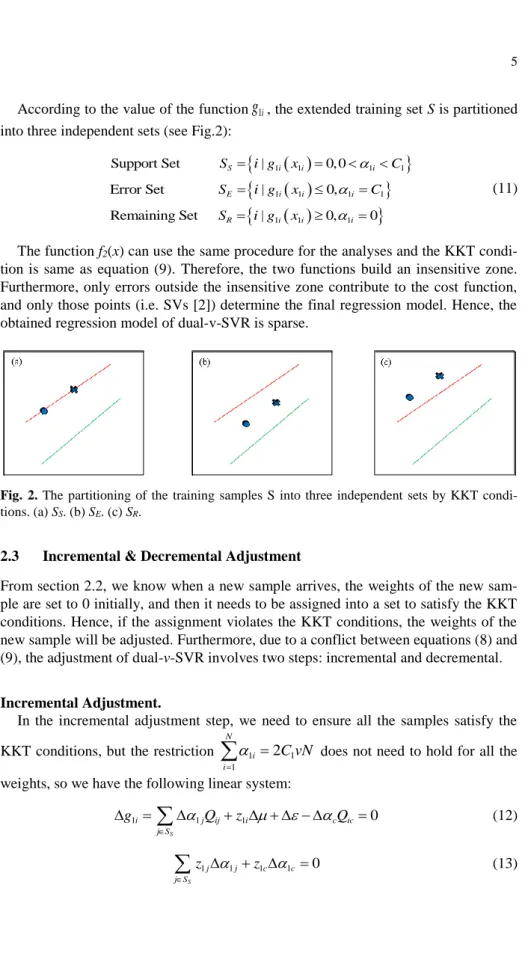
1 1 1 1 1 0 0 0 0 0 i i i for for C for C (10)According to the value of the function
g
1i, the extended training set S is partitioned into three independent sets (see Fig.2):Support Set SS
i g| 1i
x1i 0, 01iC1
Error Set SE
i g| 1i
x1i 0,1iC1
(11)
1 1 1
Remaining Set SR i g| i xi 0,i0
The function f2(x) can use the same procedure for the analyses and the KKT
condi-tion is same as equacondi-tion (9). Therefore, the two funccondi-tions build an insensitive zone. Furthermore, only errors outside the insensitive zone contribute to the cost function, and only those points (i.e. SVs [2]) determine the final regression model. Hence, the obtained regression model of dual-v-SVR is sparse.
Fig. 2. The partitioning of the training samples S into three independent sets by KKT condi-tions. (a) SS. (b) SE. (c) SR.
2.3 Incremental & Decremental Adjustment
From section 2.2, we know when a new sample arrives, the weights of the new sam-ple are set to 0 initially, and then it needs to be assigned into a set to satisfy the KKT conditions. Hence, if the assignment violates the KKT conditions, the weights of the new sample will be adjusted. Furthermore, due to a conflict between equations (8) and (9), the adjustment of dual-v-SVR involves two steps: incremental and decremental.
Incremental Adjustment.
In the incremental adjustment step, we need to ensure all the samples satisfy the KKT conditions, but the restriction 1 1
1 2 N i i C vN
does not need to hold for all the weights, so we have the following linear system:1 1 1 0 S i j ij i c ic j S g Q z Q
(12) 1 1 1 1 0 S j j c c j S z z
(13)where
1j,z
1j,
and
g
1i denote the corresponding variations. Then we define
1, ,1
S
T S
e as the
S
s dimensional column vector with all ones, let 1,S S
T
S S
z z z , and let
Q
S SS Sdenote the matrix, the above liner system can be fur-ther rewritten as:\ \ 1 1 0 z S 0 S S S S S S T S c c S S c S S S S h Q z Q e z Q (14)
where
Q
\ is the abbreviation of the matrix above the under brace,
h
\ is also the abbreviation which is defined in the same way.Let R Q\1
and 0, then the linear relationship between
h
\ and
1c can be easily solved as follows:\ 1 \ 1 S S S c c c c c S S c S z h R Q (15) where \ c
stands for the dimension corresponding to
in the vector \c
. S c S
is the vector with the same meaning of
\c . Accordingly, let
\c
0
, then therelation-ship between
h
\ and
ccan also be defined as: cc
h
(16)By substituting (15) and (16) into (12), we can get the linear relationship between
1i
g
and
c as follows: 1 1 1 1 S c c c c i j ij i ic c i c j Sg
Q
z
Q
, i S (17)Obviously
i
S
S, so we have
1ci
0
. Thus, for each incremental adjustment, we can compute the maximal increment of
1c (here denoted as
1cmax), update α, g, SS, SE, SR and the inverse matrix R, similar to the approaches in [20].In the decremental adjustment step, we gradually adjust 1i
i S
to restore theequality 1i 2 ( 1)
i S
Cv N
, so that the KKT conditions are satisfied by all the samples. For each adjustment of 1ii S
, in order to ensure all the samples satisfy the KKT conditions, the weights of the samples in SS, the Lagrange multipliers and
should also be adjusted accordingly, and these have the following linear system:1 1 1 0 S i j ij i j S g Q z
,
i
S
S (18) 1 1 0 S i j j S z
(19) 1 0 S j j S
(20)where
is the introduced variable of adjusting
i S
1i,
is any negativenum-ber, and is incorporated in (20) as an extra term. Using this extra term can pre-vent the recurrence of conflicts between equations (8) and (9). The above linear sys-tem can also be further rewritten as:
0 0 0 0 1 0 S S S S S S S T S T S S S S S S h Q z e z e Q (21) Let 1
RQ , then the linear relationship between hand
can be obtained as follows: 0 1 0 S S S S h R
(22)From equation (20), we have
i S
1i
1
, which implies that thecontrol of the adjustment of 1i
i S
is achieved by
.Finally, substituting equation (20) into equation (16), we can also get the linear re-lationship between
g
1i and
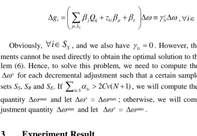
as follows:1 1 S c i j ij i i j S
g
Q
z
, i S (23)Obviously,
i
S
S, and we also have
1i0. However, the decrementaladjust-ments cannot be used directly to obtain the optimal solution to the minimization prob-lem (6). Hence, to solve this probprob-lem, we need to compute the adjustment quantity
*
for each decremental adjustment such that a certain sample migrates among the sets SS, SR and SE. If
i S
1i 2Cv N( 1), we will compute the maximal adjustmentquantity
max and let
* =
max; otherwise, we will compute the minimalad-justment quantity
min and let
* =
min.3
Experiment Result
3.1 Experiment setup
In this section, we validate the performance of the proposed incremental dual-v-SVR algorithm (IDVSVR) through several experiments which compare our algorithm with standard TSVR [22], AOSVR [9], and INSVR [12]. All regression models are imple-mented in MATLAB 2016a version on Windows 7 running on a PC with system con-figuration Intel Core i5 processor (2.40 GHz) with 8-GB RAM. We also use cadata, and Friedman data sets. Cadata [12] is a real data set, Friedman is an artificial data set [21]. The details of the three data sets are shown in Table 1.
Table 1. Data sets used in the experiments
Data set #training set # attributes
cadata 20000 8
Friedman 40000 10
For simplicity, the Gaussian radial basis function kernel is adopted for all exam-ples. We set the model parameters C1 = C2 = C and v1 = v2 = v. The values of parame-ter C, q, ε, v are, respectively, selected from the sets {10i | i = 0, 1, ... , 6}, {2i | i = −9,−8, ..., 2}, {0.01, 0.02, ..., 0.4}, and {0.01, 0.02, ..., 0.6}. As for uncertainty, as the aforementioned data sets are not noisy, we artificial introduce a noisy ei into predictor variable X and dependent variable Y, and ei is drawn from a uniform distribution on U(-k, k). Here, U(-k, k) represents the uniformly random variable in [-k, k].
3.2 Performance Evaluation
In the first experiment, we compare their trends in relation to regression risk on noisy data when the data size N is increased. We use RMSE [22] to represent the ac-curacy where a smaller RMSE represents a lower risk. Fig.3 shows the comparison result for different data sets, different data size N and different k.
(a). k=0.0, cadata (b). k=0.0, Friedman
(c). k=0.5, cadata (d). k=0.5, Friedman
(e). k=1.0, cadata (f). k=1.0, Friedman Fig. 3. Comparison result of RMSE
From Fig.3, we can see that when the data size N is increased, no matter how much k is, the RMSE of any regression is gradually decreasing. When k = 0, IDVSVR and INSVR have the better performance. These results identify that both IDVSVR and INSVR have the advantage of using parameter v to control the bounds on the fraction of SVs and errors. However, when k increases, or in other words, when the data is perturbed by noise, the IDVSVR still has the better performance, as the performance of INSVR is very poor. Furthermore, Fig.3 also shows that the accuracy of IDVSVR remains relatively stable even when k=1. Hence, a major advantage of the proposed IDVSVR over the other algorithms is its effectiveness in handling uncertain data.
In the second experiment, we compare the training speed on noisy data when the data size N is increased. In the previous experiment, we know TSVR has the worst generalization ability. Hence, we only test the training time of AOSVR, INSVR, and IDVSVR. Fig.4 shows the comparison results in terms of time for the different data sets, different data size N and different k.
(a). k=0.0, cadata (b). k=0.0, Friedman
(e). k=1.0, cadata (f). k=1.0, Friedman Fig. 4. Comparison result of training speed.
Fig.4 demonstrates that the learning speed of the IDVSVR algorithm is generally much faster than the other online SVR algorithms when data size N increases. One reason for this is that in IDVSVR, the two nonparallel functions are estimated by solving two SVR-type QPPs of smaller size at the same time, so the learning speed of IDVSVR is faster. The second reason is using an extra term to prevent the recurrence of conflicts between the equation (8) and (9) and reduce the number of adjustment. Fig.4 furthermore suggests that the prediction speed of IDVSVR model remained relatively stable in different k. But the training speed of other online SVR algorithms becomes slower with the k increased.
4
Concluding remarks
As there is no effective SVR algorithm which can handle incremental regression problem with uncertain data, we design an incremental dual-ν-SVR algorithm in this paper. Our proposed incremental dual-v-SVR has good robustness against uncertainty and can handle the incremental regression problem efficiently. Furthermore, there are a total of five advantages of our proposed incremental algorithm: (1) the learning speed of incremental dual-v-SVR algorithm is fast; (2) the sparsity of incremental dual-v-SVR algorithm is improved; (3) the incremental dual-v-SVR algorithm has good generalization performance; (4) the incremental dual-v-SVR algorithm also can use parameter v to control the bounds on the fractions of SVs and errors; and (5) in incremental dual-v-SVR algorithm, the box constraints are independent of the size of the training sample set. The experimental results also prove our conclusion.
References
1. Scholkopf, Bernhard Smola, A.J.: New Support Vector Algorithms. Neural Comput. Learn. II. 1245, 1207–1245 (1998).
2. Chang, C.-C., Lin, C.-J.: Libsvm. ACM Trans. Intell. Syst. Technol. 2, 1–27 (2011). 3. Gu, B., Sheng, V.S.: A Robust Regularization Path Algorithm for ν-Support Vector
Classi-fication. IEEE Trans. Neural Networks Learn. Syst. 28, 1241–1248 (2017).
4. Wang, G., Zhang, G., Choi, K., Lu, J.: Deep Additive Least Squares Support Vector Ma-chines for Classification With Model Transfer. IEEE Trans. Syst. Man, Cybern. Syst. 1–14 (2017).
5. Smola, A.J., B.~Schölkopf: A Tutorial on Support Vector Regression. Stat. Comput. 199– 222 (2001).
6. Shevade, S.K., Keerthi, S.S., Bhattacharyya, C., Murthy, K.R.K.: Improvements to the SMO algorithm for SVM regression. IEEE Trans. Neural Networks. 11, 1188–1193 (2000).
7. Takahashi, N., Guo, J., Nishi, T.: Global convergence of SMO algorithm for support vec-tor regression. IEEE Trans. Neural Netw. 19, 971–982 (2008).
8. Collobert, R., Williamson, R.C.: SVMTorch: Support Vector Machines for Large-Scale Regression Problems. J. Mach. Learn. Res. 1, 143–160 (2001).
9. Ma, J., Theiler, J., Perkins, S.: Accurate on-line support vector regression. Neural Com-put. 15, 2683–2703 (2003).
10. Omitaomu, O.A., Jeong, M.K., Badiru, A.B., Hines, J.W.: Online support vector regres-sion approach for the monitoring of motor shaft misalignment and feedwater flow rate. IEEE Trans. Syst. Man Cybern. Part C Appl. Rev. 37, 962–970 (2007).
11. Omitaomu, O.A., Jeong, M.K., Badiru, A.B.: Online support vector regression with var-ying parameters for time-dependent data. IEEE Trans. Syst. Man, Cybern. Part ASys-tems Humans. 41, 191–197 (2011).
12. Gu, B., Sheng, V.S., Tay, K.Y., Romano, W., Li, S.: Incremental Support Vector Learn-ing for Ordinal Regression. IEEE Trans. Neural Networks Learn. Syst. 26, 1403–1416 (2015).
13. Gu, B., Sheng, V.S., Wang, Z., Ho, D., Osman, S., Li, S.: Incremental learning for ν -Support Vector Regression. Neural Networks. 67, 140–150 (2015).
14. Hong, D.H.H.D.H., Hwang, C.H.C.: Interval regression analysis using quadratic loss sup-port vector machine. IEEE Trans. Fuzzy Syst. 13, 229–237 (2005).
15. Yang, X., Zhang, G., Lu, J., Ma, J.: A kernel fuzzy c-Means clustering-based fuzzy sup-port vector machine algorithm for classification problems with outliers or noises. IEEE Trans. Fuzzy Syst. 19, 105–115 (2011).
16. Peng, X., Chen, D., Kong, L., Xu, D.: Interval twin support vector regression algorithm for interval input-output data. Int. J. Mach. Learn. Cybern. 6, 719–732 (2015).
17. Chen, G., Zhang, X., Wang, Z.J., Li, F.: Robust support vector data description for outlier detection with noise or uncertain data. Knowledge-Based Syst. 90, 129–137 (2015). 18. Yang, X., Tan, L., He, L.: A robust least squares support vector machine for regression and
classification with noise. Neurocomputing. 140, 41–52 (2014).
19. Huang, G., Member, S., Song, S., Wu, C., You, K.: Robust Support Vector Regression for Uncertain Input and Output Data. IEEE Trans. NEURAL NETWORKS Learn. Syst. 23, 1690–1700 (2012).
20. Gu, B., Wang, J., Yu, Y., Zheng, G., Huang, Y., Xu, T.: Accurate on-line ν-support vector learning. Neural Networks. 27, 51–59 (2012).
21. Meyer, D., Leisch, F., Hornik, K.: The support vector machine under test. Neurocompu-ting. 55, 169–186 (2003).
22. Peng, X.: TSVR: An efficient Twin Support Vector Machine for regression. Neural Net-works. 23, 365–372 (2010).