Movement and Gesture Recognition Using Deep Learning
and Wearable-sensor Technology
Baao Xie, Baihua Li*, Andy Harland
Loughborough University, Loughborough, UK LE11 3TU
First Author: [email protected]
*Corresponding Author: [email protected]
ABSTRACT
Pattern recognition of time-series signals for movement and gesture analysis plays an important role in many fields as diverse as healthcare, astronomy, industry and entertainment. As a new technique in recent years, Deep Learning (DL) has made tremendous progress in computer vision and Natural Language Processing (NLP), but largely unexplored on its performance for movement and gesture recognition from noisy multi-channel sensor signals. To tackle this problem, this study was undertaken to classify diverse movements and gestures using four developed DL models: a 1-D Convolutional neural network (1-D CNN), a Recurrent neural network model with Long Short Term Memory (LSTM), a basic hybrid model containing one convolutional layer and one recurrent layer (C-RNN), and an advanced hybrid model containing three convolutional layers and three recurrent layers (3+3 C-RNN). The models will be applied on three different databases (DB) where the performances of models were compared. DB1 is the HCL dataset which includes 6 human daily activities of 30 subjects based on accelerometer and gyroscope signals. DB2 and DB3 are both based on the surface electromyography (sEMG) signal for 17 diverse movements. The evaluation and discussion for the improvements and limitations of the models were made according to the result.
Keywords
Pattern Recognition; Deep Learning; Movement Classification; Wearable-sensor; Time-series Signals Processing;
1.
INTRODUCTION
For several decades, the pattern recognition of movement and gesture shows promise for human-machine interaction in many areas. A remarkable application of movement recognition is human activity recognition (HAR). Most HAR applications are based on raw sensor inputs such as accelerometer and gyroscope signals which show its ability in learning profound knowledge about movement recognition [2]. Another potential application in this area is gesture classification for upper limb amputees which uses surface electromyography (sEMG) to capture the muscle activation as electrical signals. sEMG signals are recorded by several electrodes placed on the skin of the upper limb to detect voltage potential difference of muscle activities. Each hand movement can be treated as a class during the training process. The trained model can be applied on the applications ranging from polyarticulated prosthetic hands to entertainment interfaces.
The traditional machine learning approaches such as decision tree, support vector machine, naive Bayes, and hidden Markov models have been widely used in classification and pattern recognition tasks [3]. These conventional models give a high accuracy with large amounts of hand-crafted, structured, and under controlled data. However, traditional ML models require lengthy offline and
batch training which is not incremental or interactive for real time application. For a trained model, the testing data should be seen and labeled to produce a satisfactory result. In addition, ML models always cost a long period of time to extract a set of reliable features especially for high-dimensional, complex and noisy data because of the various situations in practical applications. It also requires a high-level domain knowledge for the hand-crafted feature extracting which lead to the poor transfer learning ability and poor re-usability. Besides the ML methodologies, recent years have witnessed the fast development and advancement of deep learning, which made significant progress in many areas such as pattern recognition and logic reasoning [1]. As a novel methodology for processing a large amount of data, DL technology makes it possible for computers via artificial intelligence to collect data, analyze data, classify data and sort out the result without hand-crafted feature extraction. The high accuracy and reliability of DL models such as Convolutional Neural Network (CNN) and Recurrent Neural Network (RNN) are proved especially in fields of image recognition, signal recognition and activity classification. The aim of this work is to develop deep learning based methods for human movement recognition from time-series signals such as obtained using sEMG and wearable sensors (IMU, accelerometers). We would like to understand the performance of DL for time-series signal analysis and accuracy, as to our knowledge, this aspect is still understudied. A series of experiments have been conducted to achieve it with different datasets and signals. The DB1 is a well-known HAR dataset from 30 subjects. The DB2 and DB3 are sub-datasets of Ninapro database contains the recordings of 17 gestures from subjects by collecting sEMG signal. There are 4 different DL models designed for the experiments to find out the optimum solution by performance comparison: a 1-D CNN, a LSTM model, a C-RNN and 3+3 C-RNN. The details of datasets and models are described in the following sections. In addition, performances and results of models are presented and analyzed. The limitations and potential improvements are discussed after the comparison of different models.
2.
RELATED WORK
Traditionally, movement and gesture recognition is based on the machine learning approaches which produce a satisfactory result with large amounts of hand-crafted and structured data. As a research of ML and signal recognition, an artificial neural network (ANN) was developed in [4] to classify the sEMG movement signals based on handcrafted features. A series of features in time-domain and frequency time-domain such as Mean Absolute Value (MAV), Root Mean Square (RMS) and Variance of EMG (VAR) were selected to train the ANN model [4]. Another application of ML in this field is mentioned in [5], which developed a support vector machine (SVM) model to train the data and give a strategy of parameter adjustment to improve controller performance [5]. Similarly, in [6], an unsupervised adaptation strategy of linear
discriminant analysis (ALDA) was developed to improve the performance of sEMG-based motion recognition. The ML models above rely on the accurate and complex hand-crafted features which require a high-level domain knowledge for researches. In the recent years, many researchers turn to DL models like CNN and RNN for a potential improvement of signal recognition. In an early work in this direction [7], the signal in each dimension of the accelerometer data is treated as the data in RGB channels of an image. Then the convolution and pooling can be applied separately in each channel. Another similar work in [8] use 1-D CNN to train the data where the single sensor input is treated as a 1-D image. The limitation of these works based on 1-D CNN is the ignored dependencies between sensors and dimension, which make a difference on the performance [2]. For the signals from multiple channels, some researchers such as [9] use 2-D CNN which regards the signals from channels as a complete image, the height of the ‘image’ is the channels of signal where the width of the ‘image’ is the time period of input signal (usually presented as a sliding window width). So that it is possible to feed multiple channels signal into an image recognition model. Besides, there are also some hybrid models of CNN and RNN. In [10], a deeper network was developed named DeepConvLSTM, which contains 4 convolution layers and 2 recurrent layers. It leads to a better performance compared to basic CNN models on HAR recognition. In addition, other researches combined CNN with different models such as restricted Boltzmann machine (RBM) [11] and Stacked autoencoder (SAE) [12]. In these compound models, CNN is used to extract features before the data go through the classifier. As a similar project in [13], Carl (2017) used 5 different classifiers on the DB3, where the Random Forest (RF) classifier performs best out of all five. The DL models used in this paper were inspired by previous works, especially the 1-D CNN and the hybrid model of different networks.
3.
METHOD
In this section, the structures of four designed models are described. In addition, section 3.3 presents more details of the advanced hybrid model.
3.1
1-D CNN
CNN is the most well-known model of DL in recent years. It is a special kind of multi-layer neural network which at the early stage was developed for image pattern recognition. CNN is able to recognize different patterns based on the features analyzed by itself [17]. The most famous CNN application on visual recognition is that in 2012, Alex Krizhevsky used them to win that year’s ImageNet competition, dropping the classification error rate from 26% to 15%. It is an outstanding improvement in this field at that time [18]. After that, more and more CNN applications in other fields such as video recognition [17], natural language processing, online photo searching and speech recognition show up in recent years. And for signal recognition, the CNN traditionally treats the multiple channels signal as a 2-D image where the height is the number of channels and the width is the sliding window size. However, the signal and image are vastly different. The features and variabilities of the signal are materialized on the time domain. Therefore, in the experiment, a 1-D CNN was designed which was inspired by [19]. The model processes separable convolution operation on each channel of the data rather than do the convolution on the entire input matrix. There are 2 convolutional layers in the model with max pooling and activation function applied after each convolution layer. The output of several separable convolution layers is the feature maps of inputs from different channels. And a
fully-connected layer will be applied on these nodes, following by the classifier to generate the result.
3.2
LSTM
As mentioned in the last section, the features of data based on time domain are significant in signal recognition. In this field, RNN shows its ability on sequence data such as speech, texts, and signals. Especially, LSTM is a powerful variation of RNN models for time-series signal recognition focusing on the relationships between the data at different time points. The features and information from previous time point are stored in a memory node of each neuron. The input and memory of current time point influence the prediction synchronously.
The RNN used in the experiment is a basic LSTM model with the sequence length of 128 which equals to the sliding window size. There is a dropout layer after the LSTM layer with problem rate of 0.8 to overcome the overfitting problem. And a fully-connected layer will be applied on these nodes, following by the classifier to generate the result.
3.3
C-RNN
The hybrid model combined with CNN and RNN for pattern recognition has become a trend in recent years. One or more convolutional layers are applied as a feature extractor in the structure. The output of the convolutional layers is the feature map of the input signal which contains useful information for other layers and the classifier. The LSTM layers focus on the influence from previous time point and generate a probability map for each input. In the early stage of the experiment, a basic C-RNN model was developed including 1 convolutional and 1 recurrent layer. After some literature reviews and modifications, another advanced C-RNN model was built with 3 convolutional layers and 3 recurrent layers. In this section, the structure of the 3+3 C-RNN is described with more details.
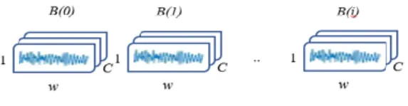
Figure 1. Input format of 3+3 C-RNN.
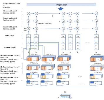
As shown in Figure 1, the input of the model should be a signal piece fixed by a sliding window. The width of the input is in the time domain, and the size equals to the window size w. The height of the signal should always be 1. C represents the number of input channels while the signal from each channel will be fed into 1-D convolutional layers separately. For one round of training, a batch of such signal piece will be fed into the network where the batch size equals to i. As Figure 2 shows, the number of filters of the 1st Conv layer is designed as C*2, with the filter size of 2 and stride size of 1. The zero-padding approach is applied after each Conv layer to generate a feature map (FM) in the same width. The output format of 1st Conv layer should be [B(i), w, C*2]. The 2nd and 3rd Conv layers are designed to have the same filter size and stride size but twice of the number of filters. The output of the 3rd Conv layer should be [B(i), w, C*8]. It is worth mentioning that, the parameters in the layers are controllable for a better performance. And different from traditional CNN, there is no max pooling layer after convolution which aims to keep the integrality of data and ensure the fixed length of the sequence to feed into LSTM layers.
Figure 2. Structure of 3+3 C-RNN.
As shown in Figure 2, the output of convolutional layers are sequences of the feature map. These feature sequences will be reshaped into a node for recurrent layers. The width of the sequence is treated as the time period of recurrent layers which equals to w. Then, a dense layer will transform these nodes and feed them into the LSTM cells, each with the dimension LSTM size (Ls). This size parameter is designed to be 3 times larger than the number of channels, which is the similar way in the embedding layers in text applications where words are embedded as vectors from a given vocabulary [20]. Then the sequence with the length of window size will be feed into three LSTM layers continuously. The input of each layer is the output from the previous layer. The dropout function is applied with problem rate of 0.8 for 1st and 2nd layers. And for the 3rd recurrent layer, the problem rate will be 0.5. In addition, the gradient clipping approach is added to improve training by preventing exploding gradients during back propagation. Only the last member of the sequence at the last LSTM layer is used as the final result, which will be feed into the fully-connected layers and a Softmax layer for classification.
3.4
DATA
This section describes the datasets and signal types used in the experiments. All the databases are public and available online.
3.4.1
Database 1
The DB1 used in the experiment is the HAR dataset from the UCI repository. The dataset is taken from with 30 subjects within an age range of 19-48 years. Each volunteer was asked to perform six movements (walking, walking upstairs, walking downstairs, sitting, standing and laying) wearing a smartphone on the waist. The accelerometers, gyroscope, and body accelerometer signals were recorded at a sampling rate of 50 Hz. The dataset was separated into two parts randomly where 70% of the set was selected as training set and 30% as the testing set. In the pre-processing step, noise filters were applied to the signals. The signals sampled in the fixed-width sliding window of 2.56 sec with 50% overlapping [14]. More details and attributes information of DB1 are available at
https://archive.ics.uci.edu/ml/index.php.
3.4.2
Database 2
The DB2 and DB3 used in the experiment are sub-datasets of Ninapro database which provides a repository of sEMG data.
sEMG measures the electrical activity when muscles are moving and exercising. It is an important attribute of the nervous systems aimed at collecting more muscular force or compensating for force losses. When measuring the movements of muscle, sEMG is reliable, but with light movements and deep muscles, sEMG collected by the wearable sensor is required for a high level of accuracy [16]. The purpose of the Ninapro project is to aid research on advanced hand myoelectric prosthetics with public datasets [15]. Currently, there are 7 databases available, each containing results from a series of movements where volunteers performed sets of hand, wrist and finger movements in controlled laboratory situations. The DB2 is the sub-dataset 5 of Ninapro database which contains data acquisitions of 10 subjects. The sEMG signals in the set were collected using two Thalmic Myo armbands with 16 electrodes, providing the upsampled sEMG signal at 200 Hz. The armbands were fixed close to the elbow according to the Ninapro standards. Each subject repeats 17 different hand movements for 6 times. Each movement lasts for 5 seconds and following by 3 seconds of rest as shown in Figure 3.
Figure 3. 17 Movements in Ninapro databases.
The subject 1-7 were treated as training set and subject 8,9,10 were selected as the testing set.
3.4.3
Database 3
The DB3 is the sub-dataset 2 of Ninapro database, which contains data acquisitions of 40 subjects. The sEMG signals in the set were collected using 12 electrodes from a Delsys Trigno Wireless System, providing the raw sEMG signal at 2 kHz. The type of movements of DB3 is same as DB2. The dataset was separated into two parts randomly where 70% of the set was selected as training set and 30% as the testing set. More details and attributes information of DB2 and DB3 are available at
http://ninapro.hevs.ch/node/7.
3.5
Evaluation
In the above sections, 3 databases and 4 DL models are described. This section contains the evaluation function and configurations of the experiments. During the testing, the average accuracy of each model is measured by a testing set with the loss function of multiclass cross-entropy as shown in (1).
𝐻(𝑝, 𝑞) = − ∑ 𝑝(𝑥) 𝑥 log 𝑞(𝑥). (1)
Multiclass cross-entropy compares two values or matrices, which present the label and prediction of the network and generate a loss of the model. Where the p(x) equals the value of label for dataset x and q(x) equals to the prediction result for dataset x. The lower loss rate means the prediction is closer to the label.
4.
RESULT
For each model, the learning rate is set at 0.0001 and the epoch size is set as 1000. The batch size is designed as 600. The training and testing are implemented on a computer with GPU of GTX 1080ti and CPU of Intel(R) Core(TM) i7-7700k @ 4.20Ghz. The programming platform is Tensorflow with python.
Table 1 shows the average accuracy of different models when applied on datasets. It is obvious that 3+3 C-RNN gives the best performance on three datasets, which are 90.29%, 83.61% and
63.74%. For the Ninapro datasets (DB2 and DB3), 1-D CNN produces an unsatisfactory result of 53.17% when compared to other models. It is clear that for these 2 datasets, the models containing LSTM layer give a better accuracy, which means the relationships between different time points have more influence on the sEMG signal recognition.
Table 1. Performance of DL models
Models DB1 DB2 DB3
1-D CNN 88% 72.49% 52.17% LSTM 86.8% 78.13% 55.3% C-RNN 87.62% 82.1% 59.31% 3+3 C-RNN 90.29% 83.61% 63.74%
However, for the HAR dataset, 4 models produce a high accuracy (above 85%). The one reason is the HAR database has fewer classes (6) than the Ninapro database (18) which makes it easier to classify. In addition, the class of ‘rest’ in Ninapro datasets seems to cause a decrease of the accuracy.
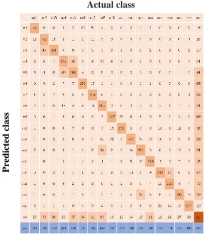
It is also worthy to mention that a large number of subjects (40 for DB3) with insufficient sample data cause a confusion for DL models and lead to a lower accuracy. Theoretically, this situation should be ameliorated if more sample data are fed to the networks. Since some researchers and organizations are interested in the performance of specific movements, the confusion matrices of 3+3 C-RNN are provided for each dataset. Each row of the matrix represents the instances in predicted movements while each column represents the instances in actual movements. Figure 5 is the confusion matrix of DB1. During the testing, 94 samples of movement 4 were classified as movement 5 and 95 samples of movement 5 were classified as movement 4. It means the 3+3 C-RNN still make mistakes between movement 4 (sitting) and movement 5 (standing) after training. In addition, the classification of movement 1 (walking) and movement 2 cause a trivial confusion for the model.
Figure 5. Confusion matrix of 3+3 C-RNN for DB1.
The confusion matrix of DB2 and DB3 shows the similar result because they based on the same dataset. Figure 6 is the confusion matrix of DB2 as an example, which contains the specific accuracy of 18 movements. The movement 0 is the pausing class which obviously cause a confusion for the 3+3 C-RNN when classifying it with other movements. The similarity of movements and pausing is mainly distributed in the early stage and the ending stage of signals.
Figure 6. Confusion matrix of 3+3 C-RNN for DB2.
5.
DISCUSSION
From the results, the DL models give a satisfactory result on DB1 and DB2 where the accuracy of DB3 is lower. The larger amount of data, the higher sampling rate, and unsuitable model strategy can be the reasons. Therefore, there is still potential to improve the DL models for a better performance.
● Hyperparameter Tuning
Hyperparameter tuning is an important approach in Model optimization for machine learning and deep learning. The parameters such as learning rate, sliding window size, and batch size make a vital influence on the performance and can be tuned to control the behavior of a DL algorithm. The window size adjustment can be a direction of improvement where the size is fixed to 128 in this stage. It seems to be reasonable to set different window size for each dataset with different sampling rate to ensure that each window contains the same amount of sample as the inputs. More experiments should be done with diverse sets of hyperparameter for a better performance.
● Dataset Strategy Adjustment
Obviously, different dataset strategy leads to the different results for models. The adjustment of data can be a potential way to improve the performance. For instance, in the DB2 and DB3, removing the class of pausing may increase the accuracy because this class causes a confusion for DL models with other movements as shown in previous sections. In addition, for the practical application, each model should be able to give a reasonable performance on unseen subjects. It is a possible optimization to use unseen dataset for testing in the experiment.
● Structure Modification
The DL model is the core of the experiment so the structure modification is another fact for improvement. For instance, the adding of dropout layer solved the overfitting problem for each model. In the future work, more functional layers can be inserted into the networks for a better result.
● Data Preprocessing
A critical difference between traditional machine learning and deep learning is the ML models use hand-crafted features as the input
Actual class Pr edi cte d cl ass Actual class Pr edi cte d cl ass
where the DL models use raw data. The ML approaches such as support vector machine and deep belief network with well-designed features give a tremendous performance in pattern recognition field. It can be a worthy trial to feed preprocessed data or hand-crafted features as the input to DL models rather than using the raw signals.
6.
CONCLUSION
Signal-based recognition is an important research area in pattern recognition and signal processing. In this paper, four different deep learning models were applied for signal recognition. The structure of each model was introduced. In the experiment, three databases were used including an IMU dataset and two EMG datasets. The 3+3 C-RNN gave the best performance over 3 datasets where the accuracy reached 90.29%, 83.61%, and 63.74%. Based on the performance result, the potential improvements were discussed in different aspects.
7.
ACKNOWLEDGMENTS
The sEMG data used in this paper are from the NinaPro project [15], we would like to express special thanks. We would also like to thank Carl Peter Robinson who provided his knowledge to support to this work.
8.
REFERENCES
[1] LeCun, Y., Bengio, Y., Hinton, G. 2015. Deep learning.
Nature 521,1 (May. 2015), 436-444.
[2] Wang, J., Chen, Y., Hao, S., Peng, X., and Hu, L. 2018. Deep Learning for Sensor-based Activity Recognition: A Survey. Pattern Recognition Letters 103,1 (Feb. 2018), 1-9. [3] Lara, O.D., Labrador, M.A. 2012. A survey on human
activity recognition using wearable sensors. IEEE Communications Surveys & Tutorials 15, 3 (Nov. 2012) 1192-1209.
[4] Ahsan, M., Ibrahimy, M., and Khalifa, O. 2011. Electromygraphy (EMG) signal-based hand gesture
recognition using artificial neural network. In Proceedings of IEEE Int. Conf on Mechatronics. (Kuala Lumpur, Malaysia). IEEE, 1-6.
[5] Oskoei, M. A. and Hu, H. 2008. Support vector machine-based classification scheme for myoelectric control applied to upper limb. IEEE Transactions on biomedical
engineering. 55, 8 (Mar. 2008), 1956-1965.
[6] Zhang, H., Zhao, Y., Yao, F., Xu, L., Shang, P., and Li, G. 2013. An adaptation strategy of using lda classifier for EMG pattern recognition. In Proceedings of 35th Annual
International Conference of the IEEE. (Osaka, Japan). IEEE, 4267-4270
[7] Zeng, M., Nguyen, L.T., Yu, B., Mengshoel, O.J., Zhu, J., Wu, P., Zhang, J. 2014. Convolutional neural networks for human activity recognition using mobile sensors. In
Proceedings of Mobile Computing, Applications and Services, 2014 6th International Conference. (Austin, TX, USA). IEEE, 197-205.
[8] Pourbabaee, B., Roshtkhari, M.J., Khorasani, K. 2017. Deep convolution neural networks and learning ecg features for screening paroxysmal atrial fibrillatio patients. IEEE Trans.
on Systems, Man, and Cybernetics, (June. 2017), 1-10. DOI: 10.1109/TSMC.2017.2705582
[9] Ha, S., Yun, J.M., Choi, S. 2015. Multi-modal convolutional neural networks for activity recognition. In Proceedings of Systems, Man, and Cybernetics (SMC), 2015 IEEE International Conference (Kowloon, China). IEEE, 3017-3022.
[10]Ordonez, F.J. and Daniel, R. 2016 Deep convolutional and LSTM recurrent neural networks for multimodal wearable activity recognition. Sensors, 16, 1 (Jan. 2016), 1-25. [11]Liu, C., Zhang, L., Liu, Z., Liu, K., Li, X., Liu, Y., 2016.
Lasagna: towards deep hierarchical understanding and searching over mobile sensing data. In Proceedings of the 22nd Annual International Conference on Mobile Computing and Networking (New York, USA). ACM, New York, NY. 334-347.
[12]Zheng, Y., Liu, Q., Chen, E., Ge, Y., Zhao, J.L. 2016. Exploiting multichannels deep convolutional neural networks for multivariate time series classification. Frontiers of Computer Science 10,1 (Feb. 2016) 96-112.
[13]Robinson, C. et al. 2017. Pattern classification of hand movements using time domain features of electromyography. In Proceedings of 4th Int. Conf Movement Computing (London, United Kingdom). MOCO ’17. ACM, New York, NY, 27:1–6.
[14]Anguita D, Ghio A, Oneto L, et al. 2013. A public domain dataset for human activity recognition using smartphones. In
Proceedings ofEuropean Symposium on Artificial Neural Networks, Computational Intelligence and Machine Learning. (Bruges, Belgium).
[15]Pizzolato, S., Tagliapietra, L., Cognolato, M., Reggiani, M., Müller, H., & Atzori, M. 2017. Comparison of six
electromyography acquisition setups on hand movement classification tasks. PloS one, 12, 10 (Oct. 2017), e0186132. [16]Allen, T. R., Brookham, R. L., Cudlip, A. C., & Dickerson,
C. R. 2013. Comparing surface and indwelling electromyographic signals of the supraspinatus and infraspinatus muscles during submaximal axial humeral rotation. Electromyogr Kinesiol, 23, 6, 1343-1349. [17]Phạm D.V. 2012. Online Handwriting Recognition Using
Multi Convolution Neural Networks. In Proceedings of Simulated Evolution and Learning. (Hanoi, Vietnam) Springer, Berlin, Heidelberg, 310-319.
[18]Deshpande, A. 2016. A Beginner's Guide to Understanding Convolutional Neural Networks. Retrieved from
https://adeshpande3.github.io/A-Beginner%27s-Guide-To-Understanding-Convolutional-Neural-Networks/
[19]Saeed, A., 2016. Implementing a CNN for Human Activity Recognition in Tensorflow. Retrieved from
https://aqibsaeed.github.io/2016-11-04-human-activity-recognition-cnn/
[20]Burakhimmetoglu. 2017. Retrieved from
https://burakhimmetoglu.com/2017/08/22/time-series-classification-with-tensorflow/