Debt stabilizing fiscal rules

WO R K I N G PA P E R S E R I E S

N O. 5 7 6 / J A N UA RY 2 0 0 6

DEBT STABILIZING

FISCAL RULES

by Philippe Michel,

In 2006 all ECB publications will feature a motif taken from the €5 banknote.

W O R K I N G PA P E R S E R I E S

N O. 5 7 6 / J A N U A RY 2 0 0 6

DEBT STABILIZING

FISCAL RULES

by Philippe Michel

,

Leopold von Thadden

and Jean-Pierre Vidal

1 We thank Roel Beetsma, Andrew Hughes Hallett, Luisa Lambertini, Eric Leeper, José Marin, Efraim Sadka, Andreas Schabert, as well

This paper can be downloaded without charge from http://www.ecb.int or from the Social Science Research Network electronic library at http://ssrn.com/abstract_id=873586.

© European Central Bank, 2006 Address

Kaiserstrasse 29

60311 Frankfurt am Main, Germany

Postal address

Postfach 16 03 19

60066 Frankfurt am Main, Germany

Telephone +49 69 1344 0 Internet http://www.ecb.int Fax +49 69 1344 6000 Telex 411 144 ecb d

All rights reserved.

Any reproduction, publication and reprint in the form of a different publication, whether printed or produced electronically, in whole or in part, is permitted only with the explicit written authorisation of the ECB or the author(s).

The views expressed in this paper do not necessarily reflect those of the European Central Bank.

C O N T E N T S

Abstract 4

Non-technical summary 5

1 Introduction 7

2 The model with exogenous labour supply 11

3 Stability under a debt targeting rule:

a common framework with three instruments 16

3.1 Underaccumulation steady states 19

3.2 Golden rule steady states 22

4 Extensions 26

4.1 Alternative representations of the

debt targeting rule 26

4.2 Endogenous labour supply and

distortionary taxes 27

4.2.1 Underaccumulation steady state 30

4.2.2 Golden rule steady state 31

5 Conclusion 32

References 33

Appendix 1: Fixed labour supply and

lump sum taxes 36

Appendix 2: Endogenous labour supply and

distortionary taxes 41

Figures 43

51

Abstract

Unstable government debt dynamics can typically be corrected by various

fiscal instruments, like appropriate adjustments in government spending, pub-lic transfers, or taxes. This paper investigates properties of state-contingent debt targeting rules which link stabilizing budgetary adjustments around a target level of long-run debt to the state of the economy. The paper es-tablishes that the size of steady-state debt is a key determinant of whether it is possible to find a rule of this type which can be implemented under all availablefiscal instruments. Specifically, considering linear feedback rules, the paper demonstrates that there may well exist a critical level of debt beyond which this is no longer possible. From an applied perspective, this finding is of particular relevance in the context of a monetary union with decentralized

fiscal policies. Depending on the level of long-run debt, there might be a

con-flict between a common fiscal framework which tracks deficit developments as a function of the state of the economy and the unrestricted choice of fiscal policy instruments at the national level.

Keywords: Fiscal regimes, Overlapping generations

Non-technical summary

In European Monetary Union the principle of subsidiarity (as laid down in Article 5 of the Treaty or Article I-9 of the draft constitution) is of key importance for the distribution of responsibilities between the union and the national member states. According to this principle, the union shall act only if and insofar as the objectives of the intended action cannot be sufficiently achieved by the member states. Applied to the field of fiscal policy this principle means that member states are responsible for their national and sub-national budgetary policies, subject to certain constraints of a common fiscal framework. Such constraints are needed to keep free-riding incentives at the national level in check. Without such constraints, an insufficient lack of fiscal discipline could undermine the smooth working of automatic fiscal stabilizers, lead to unstable government debt dynamics and ultimately result in conflicts with monetary policy. To avoid such outcomes, the common fiscal framework, which is implemented at the level of the union, monitors how broad fiscal indicators, like the deficits of member states, react to the state of the economy. Whenever corrective fiscal policy measures are needed, the framework respects, in principle, national preferences with respect to the implementation of such measures. In other words, in line with the subsidiarity principle, governments are free to correct imbalances by adjusting any revenue or expenditure component and to design their own fiscal policy reactions, provided that they are consistent with the broad requirements of the overall fiscal framework.

Motivated by these features (which are qualitatively of importance for any monetary union with decentralized fiscal policies), this paper develops a simple dynamic general equilibrium model in which governments can choose between various fiscal instruments to achieve stable debt dynamics, subject, however, to the provisions of a rule-based common framework. The model analysis is rather stylized and the broad modelling assumptions maintained in this paper cannot capture many of the institutional details which characterize the particular arrangement of fiscal policies in EMU. Yet, the paper shows that a sufficiently low level of average debt facilitates the smooth functioning of any carefully balanced arrangement of this type. By contrast, at high levels of average debt conflicts may arise between the provisions of a common fiscal framework and the unrestricted choice of fiscal policy instruments at the national level.

More specifically, the paper starts out with the observation that unstable government debt dynamics can normally be corrected by appropriate budgetary adjustments. Moreover, to achieve the needed corrections a government can typically adjust a broad range of fiscal instruments, like government spending, public transfers, or various taxes. Given this multiplicity of fiscal instruments, this paper develops the idea that there are two different ways to conceptualize state-contingent fiscal rules which stabilize government debt dynamics around a certain long-run level of debt. First, for a particular instrument one can think of rules which establish a link between

Whether it is preferable to condition the path of budgetary adjustments on the state-contingent path of a particular instrument (or a combination of various instruments) or, alternatively, to condition the choice of the instrument on a particular state-contingent path of budgetary adjustments depends on the context at hand. This paper argues that the second line of reasoning is particularly relevant for the design of fiscal rules in a monetary union with decentralized fiscal policies, in which the objectives are constrained by the common framework while the instruments are left to the choice of national governments. Specifically, it can be used to see that, depending on the target level of government debt, conflicts may arise between a common fiscal framework which imposes constraints on deficit developments and the unrestricted choice of fiscal policy instruments at the national level.

To see intuitively, why a debt targeting rule, when expressed in terms of budgetary adjustments, may not always be implementable under all instruments consider, for simple illustration purposes, a government which can generate surpluses by reducing government expenditures or alternatively by raising wage income taxes. In a life-cycle framework one can well imagine that the second measure will decrease private sector savings, while the first measure may leave savings constant. Accordingly, for any given fiscal consolidation requirement, the crowding out of private sector investments is likely to be different under the two instruments, implying that the state of the economy is likely to evolve differently under the instruments. As a result, it is a priori not clear whether for a given specification of such a debt targeting rule its implementability under both instruments will be ensured.

The paper shows that the answer to this question depends on the target level of debt around which the economy is stabilized. Considering a model economy with three distinct fiscal instruments (government consumption expenditures, transfer payments and a wage income tax), the key theoretical result of the paper states that the number of instruments which can be used to implement such a rule declines in the level of steady-state debt. Essentially, this result reflects that the model economy consists of two parts: the budget constraint of the government and a second part which summarizes all the remaining private sector activities in the economy. By construction, the source of instability is confined to the first part, while the instruments which can be used to achieve the required fiscal surpluses operate through different channels and have therefore different effects on private sector activities. The level of steady-state debt determines the relative importance of these effects within the set of intertemporal equilibrium conditions. Under a low level of steady-state debt, these effects carry low weights, making it possible that the debt targeting rule can be implemented with a common set of feedback coefficients under all three instruments. With high debt, however, the strength of these effects increases, and, as debt rises, the between budgetary adjustments and the state of the economy. This second reasoning leads to the question under which instruments a particular specification of such a rule can be implemented.

1

Introduction

Unstable government debt dynamics can typically be corrected by appropriate bud-getary adjustments. To achieve the needed corrections a government can normally adjust a broad range of fiscal instruments, like government spending, public trans-fers, or various taxes. Given the multiplicity of fiscal instruments, this paper builds on the idea that there are two different ways to conceptualize state-contingent fi s-cal rules which stabilize government debt dynamics around a certain long-run level of debt. First, for a particular instrument one can think of rules which link the use of this instrument to the state of the economy. Keeping the other instruments constant, any such rule then implies a certain sequence of budgetary adjustments. Alternatively, one can think of rules which, following the reverse logic, leave the choice of the instrument a priori open and specify directly a state-contingent path of budgetary adjustments. This second reasoning leads then to the question under which of the available instruments a particular specification of such a rule can be implemented.

These two approaches, while algebraically being closely related, offer different in-sights. This paper argues that the second approach is particularly relevant for the design of fiscal rules in a monetary union with decentralized fiscal policies. Specif-ically, the logic of the second approach can be used to see that, depending on the target level of government debt, it may not be possible to find a state-contingent prescription of stabilizing budgetary adjustments that can be implemented under all available instruments. In other words, the paper argues that, depending on the target level of government debt, conflicts may arise between a commonfiscal frame-work which tracks deficit developments as a function of the state of the economy and the unrestricted choice of fiscal policy instruments at the national level.

To make this reasoning precise, this paper considers a small and fully tractable model which distinguishes between three distinct fiscal instruments in the govern-ment’sflow budget constraint, namely government consumption, transfer payments and a wage income tax. The analysis is based on a deterministic overlapping gener-ations economy with government debt dynamics in the spirit of Diamond (1965). To operationalize the notion of unstable government debt dynamics, the paper identifies steady states which are characterized by non-negative levels of government debt and which are locally unstable under the assumption of a permanently balanced primary budget. However, the economy can be stabilized at the corresponding steady-state levels if one allows for appropriate budgetary adjustments. Such adjustments can be brought about by any of the three instruments. For the sake of simple tractability, the paper considers for each instrument a rule which sets the instrument as a linear function of the two state variables of the model, physical capital and real govern-ment bonds. For given feedback coefficients associated with the two states of the economy, any such rule, when combined with the linearized flow budget constraint

of the government, generates a ‘debt targeting rule’ which specifies a particular lin-ear reaction of the primary balance to the two states of the economy. In sum, this experiment leads to a broad class of debt targeting rules, defined over the set of admissible feedback coefficients.

In line with the motivation of the opening paragraph, this class of debt targeting rules can be investigated in two directions. First, we derive for each instrument the range of instrument-specific feedback coefficients which stabilize government debt at the target value. When considered in isolation such ranges are shown to exist for all instruments. Second, we follow the reverse logic and establish whether there exists a debt targeting rule which can be implemented under all instruments

with common feedback coefficients. This amounts to check whether the ranges

of stabilizing feedback coefficients induced by the three instruments do overlap. The paper shows that the answer to this question is not trivial and depends on the level of long-run debt around which the economy is stabilized. Specifically, the key theoretical results of the paper state that at a zero level of steady-state debt there always exists a debt targeting rule which can be implemented under all three instruments with common feedback coefficients. As the level of steady-state debt rises, however, the instrument-specific adjustment paths become increasingly diverse. As we show, this feature implies that there may well exist a critical long-run level of debt beyond which there exists no longer a debt targeting rule that is implementable under all three instruments with common feedback coefficients. The novelty of these results can be assessed from different angles. First, the re-sults relate to the literature on fiscal closure rules, as typically used in large scale macroeconomic models. In this literature it is widely understood that different in-struments, when residually used to enforce the intertemporal budget constraint of the government, lead to different dynamic outcomes which preclude simple compar-isons across simulations, as discussed in Bryant and Zhang (1996), Mitchell et al. (2000), and Pérez and Hiebert (2002). Yet, by construction, this literature offers few explicit analytical findings and we are not aware of a systematic discussion of the role of government debt in this context.

Turning to tractable small scale models, stability features of Diamond-models have been discussed in a number of studies, but typically not with the intention to com-pare between the stabilization properties of different fiscal instruments.1 _More

1_{For a detailed discussion of dynamic equilibria in Diamond-models with production, but}

with-out government debt, see Galor and Ryder (1989). For comprehensive surveys of the dynamics

with debt and with zero (and, more generally, constant) primary deficits, see Azariadis (1993), and

de la Croix and Michel (2002). Special features of constant deficit rules are discussed by Farmer

(1986), with a focus on cyclical adjustment patterns, and Chalk (2000), with a focus on sustain-ability issues. For a comparison of adjustment dynamics under a balanced primary budget and a time-varying unbalanced budget, stressing labour market aspects, see Kaas and von Thadden

closely related to the spirit of this paper, Schmitt-Grohé and Uribe (1997), Guo and Harrison (2004), and Giannitsarou (2004), all considering Ramsey economies with infinitely lived agents, show that for a given fiscal rule (in their context: a balanced-budget rule) equilibria can be locally unique or indeterminate, depending on whether budget balance is achieved by distortionary income taxes, consumption taxes or government spending adjustments. Our paper shares with these papers the descriptive nature of the fiscal rule, but our focus is not on balanced budget dynamics and the role of debt is substantially different.2

Implementation issues of fiscal policy have also been addressed in a large number of papers which explicitly solve for optimal fiscal (and monetary) policies from the perspective of Ramsey economies.3 _{In such modelling environments, however, there}

is little conceptual agreement about the optimal target level of long-run debt it-self.4 _{Reflecting this feature, recent studies by Kollmann (2004), Lambertini (2004)}

and Schmitt-Grohé and Uribe (2004), for example, consider only a restricted set of optimal policies, in the sense that the long-run level of debt around which the optimization takes place is pre-specified. By contrast, the long-run target levels of government debt analyzed in our overlapping generations structure have a simple normative foundation because of dynamic efficiency considerations.5

Why may it not always be possible in our set-up tofind a state-contingent prescrip-tion of stabilizing budgetary adjustments that can be implemented under all avail-able instruments? Intuitively, this finding reflects that the model economy consists of two parts: the budget constraint of the government and a block which summa-rizes all the remaining private sector activities in the economy. By construction, the source of instability is confined to the first part, while the instruments which can be used to achieve the required budgetary adjustments affect the second part

Annicchiarico and Giammarioli (2004) and Fernandez Huertas-Moraga and Vidal (2004).

2_{Related to this literature, see also the dynamic analysis of tax changes in Judd (1987),}

Turnovsky (1990) and Mankiw and Weinzierl (2004). However, these papers do not explicitly

focus on the stabilization properties of different fiscal instruments, but rather compare between

short- and long-run features of equilibria which are characterized by different tax structures.

3_{This literature goes back to Lucas and Stokey (1983). For recent authoritative treatments,}

see, in particular, Chari and Kehoe (1999) and Benigno and Woodford (2003).

4_{In the framework of Aiyagari et al. (2002) the optimal long-run level of government debt}

is shown to be negative because of the non-distortionary nature of the interest income that a

government receives in such a constellation. Benefits of positive government debt, like the loosening

of private sector borrowing constraints because of an enhanced liquidity position, are discussed in

Aiyagari and McGrattan (1998). Costs and benefits of long-run debt levels are also discussed in

Martin (2004), with a focus on time consistency issues in the presence of non-indexed government debt. Similarly, see Díaz-Giménez et al. (2004).

5_{We do not optimize over the feedback coefficients in the debt targeting rule. The studies by}

Schmitt-Grohé and Uribe as well as by Kollmann show that simple feedback rules may well have welfare properties similar to those one obtains from fully optimizing programs. Whether a similar claim can be made in this context for overlapping generations economies needs to be investigated.

through different margins. The level of steady-state debt determines the relative im-portance of these margins within the set of intertemporal equilibrium conditions. At a zero level of steady-state debt, these margins carry zero weights, ensuring thereby that there always exists a debt targeting rule which can be implemented under all three instruments. For positive and rising levels of steady-state debt, however, these margins gain importance, implying that for any particular debt targeting rule the instrument-specific stabilization profiles become increasingly distinct. Exploiting this feature, we show that there may well exist a critical debt level beyond which it is no longer possible to find a debt targeting rule that can be implemented under all three instruments.

We think that one particularly interesting application of our results is given by mon-etary unions in which member states remain responsible for their national budgmon-etary policies, subject to the provisions of a common fiscal framework that are needed to keep free-riding incentives at the national level in check. The European Monetary Union is a good example for this since the Treaty and the Stability and Growth Pact constitute a rule-based fiscal framework that sets certain limits to deficits and debt levels and strengthens multilateral budgetary surveillance.6 _{Moreover, whenever}

corrective fiscal policy measures are needed the framework respects, in principle, national preferences with respect to the implementation of such measures, in line with the subsidiarity principle.7 _{Evidently, the broad modelling assumptions}

main-tained in this paper cannot fully capture further institutional details which charac-terize this particular arrangement. Yet, the analysis of this paper clearly indicates that a sufficiently low level of average debt facilitates the smooth functioning of any carefully balanced arrangement of this type.

The paper is organized as follows. As a particularly tractable starting point, Section

2presents a Diamond-type overlapping generations model with an exogenous labour supply, enriched with a government sector and public debt. The model allows for three fiscal instruments, namely government consumption, lump-sum taxes levied on young agents and lump-sum transfers to old agents. Section 3 introduces the notion of the debt targeting rule and derives the main results of the paper. Section

4 establishes the robustness of the main results of Section 3 along two dimensions. 6_{The main arguments forfiscal rules are: i) dynamic time inconsistency issues of (fiscal)}

policy-making, similar to that of politically dependent central banks; ii) irrationality of voters triggering political business cycles (myopic behaviour orfiscal illusion); iii) political polarization and strategic

considerations of parties alternating in office and attempting to bind the hands of their successors;

iv) common-pool problems and strategic interactions specific to monetary unions. For a recent

review of theoretical arguments in favour of a rule-based fiscal framework in a monetary union,

see Calmfors (2005). See also for further references on this widely studied topic Chari and Kehoe (2004), Fatás et al. (2003), and Uhlig (2002).

7_{According to the subsidiarity principle, as laid down in Article 5 of the Treaty (and Article I-9}

of the draft Constitution), the Union shall act only if and insofar as the objectives of the intended

First, we show that our results remain unaffected if the debt targeting rule is no longer expressed in terms of state-contingent adjustments of the primary balance, but imposes instead state-contingent restrictions on the path of the overall deficit or, alternatively, on the path of newly emitted debt. Second, at the expense of more tedious algebra, we allow for an endogenous labour supply and distortionary income taxation. This modification, while mitigating some of the effects, does not change qualitatively any of our results. Section 5 offers conclusions. Proofs and some technical issues are delegated to two Appendices at the end of the paper.

2

The model with exogenous labour supply

For simple tractability thefirst part of the paper is based on a version of a Diamond-type overlapping generations economy with exogenous labour supply and lump-sum taxes and transfers.

Problem of the representative agent

In period t, the economy is populated by a large number Nt of young agents and

Nt−1 of old agents. Each agent lives for two period and has a time-invariant, fixed

labour supply l = 1 when being young and a zero labour supply when being old. The population grows at the constant rate n > 0, i.e. Nt = (1 + n)· Nt−1. Let

preferences of the representative agent born in period t be given by

U(ct, dt+1),

where ct anddt+1 denotefirst-period and second-period consumption, respectively.

(A 1) The function U(c, d) is twice continuously differentiable, strictly increas-ing, strictly quasi-concave and satisfies for all c, d > 0, limc→0Uc(c, d) → ∞ and

limd→0Ud(c, d)→ ∞.

In any periodt,agents take the wage rate (wt) and the return factorRt+1 on savings

(st) as given. There exists a tax-transfer-system such that young agents pay

lump-sum taxes ηt >0,while they receive lump-sum transfersθt+1 when being old.8 This

leads to the pair of budget constraints

wt−ηt = ct+st

dt+1 = Rt+1st+θt+1,

which can be used to rewrite the objective as:

U(wt−ηt−st, Rt+1st+θt+1).

8_{We do not make any explicit sign restrictions regarding the second-period lump-sum payment}

The optimal choice of savings is characterized by the first-order condition

U1 =Rt+1U2.

To characterize the savings decision of agents we refer to the well-investigated Dia-mond model without second-period transfers (i.e. θt+1 = 0) and assume w−η >0.

Then, according to (A 1), there exists the savings function

s(w₋η, R) = arg maxU(w₋η₋s, Rs), (1) with s(w₋η, R) :R++×R++→R++ being continuously differentiable. In order to

extend (1) to a situation with θt+1 6= 0 it is assumed that the present value of the

income of agents is positive, i.e. w₋η+ _Rθ >0. Then, savings will be given by

st=s(wt−ηt+ θt+1 Rt+1 , Rt+1)− θt+1 Rt+1 , and st satisfies − θt+1

Rt+1 < st < wt−ηt, ensuring non-negative consumption in both

periods.9 _{Finally, to impose further structure on the function s(w, R), we make the}

customary assumption:

(A 2) ConsiderU(c, d) and assume that consumption goods are normal and gross substitutes. Then, 0< sw <1andsR≥0.

Production

It is assumed that there exists a larger number of competitive firms with access to a standard neoclassical technology F(Kt, Lt), where K andLdenote the aggregate

levels of physical capital and labour, respectively.

(A 3)The functionF(K, L) :R++×R++→R++is positive valued, twice

continu-ously differentiable, homogenous of degree 1, increasing and satisfiesFKK(K, L)<0.

Firms are price takers in input and output markets. In a competitive equilibrium, labour market clearing requires Lt = Nt. Let kt =Kt/Nt denote the capital stock

per young agent, giving rise to the familiar pair of first-order conditions

Rt = 1−δ+FK(kt,1) =R(kt) (2)

wt = FL(kt,1) =w(kt), (3)

with δ denoting the depreciation rate on capital. According to (2) and (3), the equilibrium return rates of the two production factors depend only on the equi-librium capital intensity and change along the factor price frontier with R0_(k

t) =

FKK(kt,1)<0 andw0(kt) =FLK(kt,1)>0.

9_{For a more detailed discussion of the savings problem under second-period lump-sum payments,}

Government

In the representative periodt, the government consumes an amountGt of aggregate

output which does not affect the utility of consumers.10 Let

Πt =Ntηt−Nt−1θt−Gt

denote the aggregate primary surplus. In intensive form this reads as

πt=ηt−

θt

1 +n−gt

wheregtandπtdenote government consumption and the primary surplus per young

individual, respectively. It is assumed that agents perceive investments in physical capital and government bonds (in real terms) as perfect substitutes with identical return factorRt.Then, theflow budget constraint of the government, expressed per

young agent, reads as

(1 +n)bt+1 =R(kt)bt−πt.

Intertemporal equilibrium conditions

In sum, we obtain a version of the intertemporal equilibrium conditions of the Diamond-model, modified for the existence of a simple tax-transfer system and the possibility of a primary balance that does not have to be balanced in every period

(1 +n)(kt+1+bt+1) = st=s(w(kt)−ηt+ θt+1 R(kt+1) , R(kt+1))− θt+1 R(kt+1) (4) (1 +n)bt+1 = R(kt)bt−πt (5) πt = ηt− θt 1 +n−gt. (6) Initial conditions

In each periodt,the state of the economy is summarized by the pair(bt,kt),denoting

the beginning-of-period per capita values of the capital stock and of real government bond holdings which are predetermined by past investment decisions undertaken in period t −1. Hence, when we subsequently classify the dynamic behaviour of the system (4)-(6) under various fiscal closures, it is natural to assume that dynamics are characterized by two initial conditions, b0 andk0.11

10_{If publicly provided public goods enter the utility of the representative consumer in an}

addi-tively separable manner, they do not affect the consumer’s saving decision. Our analysis would

still hold under this assumption.

11_{Note, however, that there is also a branch of the literature which stresses the role of bubbles}

in closely related models and treats real government debt as a jumping variable, see Tirole (1985). More recently, the treatment of real government debt as a jumping variable plays also a key role

Dynamics under a permanently balanced primary budget

The equations (4)-(6), without further restrictions, allow for a rich set of dynamic equilibria. In the remainder of this paper, however, we focus on the local stability behaviour of the system around steady states which have the particular feature of a balanced primary budget (i.e. π = 0). Moreover, to set the stage for a meaning-ful discussion of stabilizing off-steady-state adjustments in the primary balance in Section 3, we establish benchmark steady states of (4)-(6) which, assuming b0 6= b

and k0 6= k, are locally unstable if the primary budget is permanently balanced,

i.e. if πt ≡ 0 for all t. Specifically, consider a stationary tax-transfer system with

g _≡η₋ θ

1+n >0,leading to the two-dimensional dynamic system in kt andbt

(1 +n)(kt+1+bt+1) = st =s(w(kt)−η+ θ R(kt+1) , R(kt+1))− θ R(kt+1) (7) (1 +n)bt+1 = R(kt)bt. (8)

Using a first-order approximation, dynamics around steady states of (7) and (8) evolve according to A1·dkt+1+ (1 +n)·dbt+1 = A2·dkt (9) (1 +n)_·dbt+1 = R0(k)b·dkt+R(k)·dbt, with: (10) A1 = 1 +n−R0(k)·[sR+ (1−sw) θ R(k)2] (11) A2 = sww0(k)>0 (12)

Existence and stability conditions of steady states of (7) and (8) have been widely discussed in the literature. In particular, under mild assumptions the system is associated with two distinct types of steady states which are unstable under a per-manently balanced primary budget: i) steady states with zero debt and underaccu-mulation (k >0, b= 0, R(k)>1 +n) and ii)golden rule steady states with positive debt (k >0, bgr >0, R(k) = 1 +n). To this end, we make the assumption

(A 4) There exist steady states of (7) and (8) with k > 0 and b _≥ 0, satisfying

A2 < A1.

Remark: Assumption (A 4) is not very restrictive. For illustration, assume first

g = η = θ = 0. Then, if assumptions (A 1)-(A 3) are satisfied and, for example, the aggregate production function is of Cobb-Douglas type, there exists a unique steady state with k >0 andb= 0,satisfyingA2 < A1.12 Moreover, if at this steady

12_{If the production function is of the more general CES-type this reasoning extends to the case}

of an elasticity of substitution larger than one. If the elasticity is less than one, there are zero or two steady states with k >0andb = 0. In the latter case, the high activity steady state satisfies

state R(k) < 1 +n, there exists a golden rule steady state with k > 0, b > 0 and

R(k) = 1 +n, also satisfyingA2 < A1.Ifg =η >0andθ = 0,this reasoning can be

extended as long as g is smaller than some positive boundg. Finally, by continuity, if g _≡ η₋ θ

1+n > 0 and θ 6= 0, such steady states continue to exist as long as θ is

sufficiently small.13

From a normative perspective, the two mentioned steady-state types are relevant benchmarks because of dynamic efficiency considerations. For further reference, we conclude this section with a brief discussion of why these steady states are locally unstable. In general, according to the linearized system (9)-(10), dynamics without government debt dynamics are stable if A2 < A1, as ensured by (A 4). In the

presence of government debt dynamics, however, instability can occur because of two partial effects. First, assuming a constant interest rate (R0(k) = 0), interest payments induce a snowball effect on debt, and this effect is unstable whenever the interest rate is higher than the (population) growth rate of the economy, i.e. whenever R(k)>1 +n. Second, out of steady state the interest rate does not stay constant in an economy with capital stock dynamics, implying that, for any initial level of debt, there is an additional effect on debt according to R0_(k)b·dk

t. Any

crowding out of capital leads over time to a higher interest rate which reinforces debt dynamics. We call this second channel the interest rate effect on debt.

Benchmark 1: Underaccumulation steady state (k >0, b= 0, R(k)>1 +n)

Sinceb= 0,the interest rate effect on debt in the linearized dynamics is zero and the instability is entirely caused by the snowball effect. Because of the absence of the interest rate effect, government debt dynamics are independent of (9) and it is easy to verify that the two eigenvalues of (9) and (10) are given by λ1 =A2/A1 ∈(0,1),

andλ2 =R(k)/1 +n >1.This pattern of eigenvalues implies that, for initial values

k0 6= k andb0 6= 0 close to the steady state, dynamics are locally unstable under a

balanced primary budget rule.

Benchmark 2: Golden rule steady state (k >0, bgr >0, R(k) = 1 +n)

At the golden rule steady state with positive debt, the snowball effect is associated with a unit root, and strict instability is ensured by the additionally operating interest rate effect on debt. This can be verified from the characteristic polynomial associated with (9) and (10), evaluated at the golden rule steady state:

p(λ) =λ2₋[1 + A2 A1 − R0(k)·bgr A1 ]_·λ+A2 A1 .

13_{For a detailed discussion of the existence and stability of dynamic equilibria in Diamond-models}

with zero primary deficits, see the references quoted in footnote1. Specifically, de la Croix and

Then,p(0) =A2/A1 ∈(0,1)andp(1) =R0(k)bgr/A1 <0,implying0< λ1 <1< λ2.

Hence, at the golden rule steady state with bgr > 0 dynamics are locally unstable

under a balanced primary budget rule.

3

Stability under a debt targeting rule: a

com-mon framework with three instruments

Compared with the analysis of the previous section, we now allow for adjustments in the primary balance with the idea to stabilize the benchmark steady states, i.e.

πt 6= 0 is admitted for the off-steady-state dynamics. For a generic discussion of

such stabilizing adjustments it seems natural to think of state-contingentfiscal rules which link the variations inπt to deviations of the two state variablesbt andkt from

their steady-state values, as given by

πt =π(kt−k, bt−b), with: π(0,0) = 0.

In combination with the budget constraint of the government, appropriate rules of this type give rise to the expression

(1 +n)_·bt+1 =R(kt)bt−π(kt−k, bt−b), (13)

which, in contrast to the budget identity (5), describes a genericdebt targeting rule

which aims to stabilize the economy at the benchmark steady states. To opera-tionalize (13), the use of at least one of the three instruments needs to be linked to the states of the economy. In the following, we distinguish between three scenarios in which adjustments are achieved by variations of one of the three available fiscal instrumentsgt, ηt orθt+1,while holding the other two instruments constant at their

steady-state values.

For simplicity, we assume in all scenarios that the instruments are set as a linear function of the states. According to (6), this implies that the primary surplus πt

will also be linear in the two states.14 _{Hence, (13) can be written as}

(1 +n)_·bt+1 =R(kt)bt−πk(kt−k)−πb(bt−b), (14)

where (14) describes a broad class of debt targeting rules, parametrized by the pair of linear feedback coefficientsπkandπb.For further reference, we summarize briefly

these three scenarios, all of them being consistent with (14). 14_{In the generalized version of the model in Section4.2., tax revenuesη}

tare no longer lump sum,

but the product of a tax rate and the tax base which itself depends on the states of the economy.

Then, assuming a linear instrument rule, the coefficientsπkandπbsummarize the induced reaction

Instrument 1 : Variations in government spending gt

Assume the government satisfies (14) by adjusting government spending, according togt−g =−πt.15 Then, the intertemporal equilibrium conditions can be summarized

as (1 +n)(kt+1+bt+1) = s(w(kt)−η+ θ R(kt+1) , R(kt+1))− θ R(kt+1) (15) (1 +n)_·bt+1 = R(kt)bt−πk(kt−k)−πb(bt−b) (16) gt = eg(kt, bt) =g−πk(kt−k)−πb(bt−b) (17)

Importantly, adjustments in the primary balance via variations in gt do not affect

the accumulation equation, i.e. (15) is identical to (4). In other words, variations in gt offer a particularly convenient, non-distortionary channel to stabilize the

two-dimensional benchmark system (7)-(8). Since (17) does not feed back into the first equation the linearized dynamics read as

A1·dkt+1+ (1 +n)·dbt+1 = A2·dkt (18)

(1 +n)_·dbt+1 = (R0(k)b−πk)·dkt+ (R(k)−πb)·dbt (19)

Instrument 2 : Variations in lump-sum taxes η_t

We assume now, alternatively, that the government satisfies (14) by adjustingfi rst-period lump-sum taxes such that ηt−η =πt. Then, the intertemporal equilibrium

evolves according to (1 +n)(kt+1+bt+1) = s(w(kt)−eη(kt, bt) + θ R(kt+1) , R(kt+1))− θ R(kt+1) (20) (1 +n)bt+1 = R(kt)bt−πk(kt−k)−πb(bt−b) (21) η_t = _eη(kt, bt) =η+πk(kt−k) +πb(bt−b)

Again, dynamics are two-dimensional in kt andbt but adjustments in the primary

balance via variations in ηt do affect the disposable income of young agents and,

hence, the accumulation equation. Linearization of (20)-(21) yields

A1·dkt+1+ (1 +n)·dbt+1 = (A2−swπk)·dkt−swπb·dbt (22)

(1 +n)_·dbt+1 = (R0(k)b−πk)·dkt+ (R(k)−πb)·dbt, (23)

where the link between the instrument and the accumulation equation is captured by the use of the partial derivatives eηk =πk andeηb =πb.

15_{Primary surpluses requireg}

t< g.Recall the assumption ofg >0.In the following, we assume

thatgis sufficiently positive such that for the local dynamics around the steady state the inequality

Instrument 3 : Variations in transfers θt+1

Finally, we consider the case where the government satisfies (14) by adjusting second-period transfers such that θt+1 −θ = −(1 +n)πt+1. Then, the intertemporal

equi-librium conditions are given by

(1 +n)(kt+1+bt+1) = s(w(kt)−η+ eθ(kt+1, bt+1) R(kt+1) , R(kt+1))− eθ(kt+1, bt+1) R(kt+1) (24) (1 +n)_·bt+1 = R(kt)bt−πk(kt−k)−πb(bt−b) (25) θt+1 = eθ(kt+1, bt+1) =θ−(1 +n)·[πk(kt+1−k) +πb(bt+1−b)]

Variations in θt+1 affect the second-period disposable income of agents and, hence,

the accumulation equation. This is reflected in the linearized versions of (24) and (25) [A1−(1−sw) (1 +n) R(k) πk]·dkt+1+ [1 +n−(1−sw) (1 +n) R(k) πb]·dbt+1 =A2·dkt (26) (1 +n)_·dbt+1 = (R0(k)b−πk)·dkt+ (R(k)−πb)·dbt, (27)

where we have usedeθk =−(1 +n)πk andeθb =−(1 +n)πb.

In line with the motivation of the introduction, these three scenarios can be inves-tigated in two directions. First, for any of the two benchmark steady states it is possible to derive three instrument-specific sets of feedback coefficients πk and πb

which ensure locally stable dynamics. A simple geometric representation of these sets can be achieved if one recognizes that for each instrument the linearized local dynamics around any steady state are two-dimensional in kt and bt, giving rise to

characteristic polynomials p(λ)i, i=g, η, θ, and that stability requires

p(1)_|i >0, p(₋1)_|i >0, p(0)_|i <1, with: i=g, η, θ.

As illustrated below, for each instrument these constraints (at equality) have at any steady state a linear representation in πb − πk−space, giving rise to

instrument-specific stability regions. Intuitively, it is clear that these three regions are not identical, since variations in gt leave the intertemporal accumulation equation (15)

unaffected, while variations in η_t and θt+1 affect this equation through different

margins, as to be inferred from (20) and (24).

Second, it can be investigated whether there exists a particular debt targeting rule, characterized by a particular pair of πk and πb, which can be implemented under

all instruments. This amounts to check whether the regions of stabilizing feedback coefficients associated with the three instruments do overlap. Whenever this is the case such a debt targeting rule may be considered as the basis of a common fiscal

framework. Loosely speaking, under such a framework there are no tensions between stabilization issues and the unrestricted choice of fiscal instruments. As shown in the following two subsections, such a common framework may not always exist, depending on the characteristics of the particular steady state under consideration.

3.1

Underaccumulation steady states

This subsection shows that underaccumulation steady states, as derived in Section

2, have the particular feature that, without imposing further restrictions, all three instrument-specific sets of stabilizing feedback coefficients have a common intersec-tion. This feature is directly linked to the absence of the interest rate effect on debt at this steady state, i.e. since b = 0 any deviation of the capital stock from its steady-state value does not have by itself destabilizing effects on government debt dynamics. In other words, the instability of debt dynamics comes entirely from the snowball effect which can be fully corrected by an appropriate choice ofπb.

Accord-ingly, for all three instruments, if the debt targeting rule is characterized by πk = 0

government debt dynamics are independent of the accumulation equation and for all three linearized dynamic systems the two eigenvalues are identically given by

λ1 =A2/A1 ∈(0,1), λ2 =

R(k)₋πb

1 +n ,

as one can directly infer from the three systems (18) and (19), (22) and (23), and (26) and (27), respectively. Evidently, if πk = 0 and πb ∈ (R(k)−(1 +n), R(k) +

1 + n) dynamics will be locally stable under all three instruments. Moreover, if one considers the subset characterized by πk = 0 and πb ∈ (R(k)−(1 +n), R(k))

dynamics will not only be locally stable but also exhibit monotone adjustment for all three instruments. This reasoning leads to

Proposition 1 Consider the three instrument-specific sets of feedback coefficients

πk and πb which ensure local stability at the underaccumulation steady state under

the debt targeting rule (14). These three sets have a joint intersection, i.e. there exist values for πk andπb such that the debt targeting rule can be implemented under

all three instruments with a common set of feedback coefficients. Moreover, for some

values in the joint intersection local adjustment dynamics are monotone under all three instruments.

Proposition 1 is not confined, however, to the special assumption of πk = 0.

Gen-erally speaking, whenever πk 6= 0 this creates a policy-induced interdependence

between capital stock dynamics and government debt dynamics. This interdepen-dence differs between the three instruments. Yet, a debt targeting rule with πk 6= 0

may nevertheless be implementable under all three instruments. To demonstrate this we turn now to a more detailed discussion of the instrument-specific stability regions and consider for illustration

Example 1: F(K, L) =zKα_L1−α_{, U(c, d) =φlnc+βlnd}

δ = 1, z= 15, α= 0.4, φ= 1, β = 0.5 (i.e. sw =β/(φ+β) = 1/3), η=−θ= 2.91,

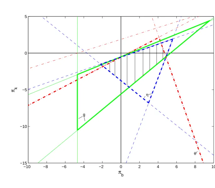
g = 4.1,1 +n= 2.43. Assuming a period length of 30 years, this implies an annual population growth of0.03.Assumingb= 0,one obtainsR= 6.29which corresponds to an annual real interest rate of0.06,consistent with an underaccumulation steady state, i.e. R(k)>1 +n. Moreover, k= 0.92, y = 14.53,where y denotes per capita output, leading to g/y = 0.28, η/y = 0.2, θ/y = ₋0.2, i.e. agents have a similar steady-state tax burden in both periods, measured in terms of per capita output. It is instructive to discussfirst in some detail the stabilizing variations in government spending gt because of their non-distortionary character. Illustrating Example 1,

Figure 1a plots the stability region in πb −πk−space for adjustments in gt. Points

inside the triangle in bold line are associated with two stable eigenvalues. The first dynamic benchmark of a permanently balanced primary budget discussed in the previous section has coordinates πb = πk = 0 and lies, by construction, outside

the stability triangle. The triangle reflects that there are potentially two margins for stabilizing adjustments of the primary balance, πb andπk, which can be used in

isolation or in combination. To further understand the shape of the triangle depicted in Figure 1a it is important to realize that there is one key difference between these two channels. Specifically, in the vicinity of any underaccumulation steady state with k0 6= k and b0 6= 0, only debt imbalances, because of the snowball effect,

destabilize on impact government debt dynamics, and consolidations according to

πb react immediately to this instability. By contrast, consolidations according to

πk respond with the delay of one period to the snowball effect and only to the

extent that it leads to the crowding out of capital. Because of the different timing of the reactions under the two channels, stabilization can always be achieved if the primary surplus exclusively reacts to the debt imbalance, i.e. ifπk = 0local stability

is ensured ifπb ∈(R(k)−(1 +n), R(k) + 1 +n)). By contrast, if the primary surplus

exclusively reacts to the capital stock imbalance stabilization may not be possible, i.e. if πb = 0 there may not exist a range forπk such that local stability is ensured,

as illustrated in Figure 1a.16 _{Hence, the effectiveness of the two fiscal feedback}

16_{However, this finding depends on the strength of the snowball effect. To further illustrate}

this, consider example1and assume, everything else being equal, α= 1/3.Because of the higher

wage income share this induces, ceteris paribus, higher savings and at b= 0 a lower return factor

R= 4.35, implying an annual real interest rate of0.05,i.e. the snowball effect will be smaller than in example 1. Then, R₋A1/A2(1 +n)<0, and full stabilization can be achieved if πb = 0 and

ifπk takes on appropriate negative values. Apart from the leftward shift of the stability triangle,

margins, when considered in isolation, is different, reflecting the general principle that, from a stabilization perspective, imbalances should be addressed directly at their source rather than indirectly and with some delay.

In any case, there exists a wide range of combinations of the two feedbacks which are consistent with locally stable dynamics. In particular, assume that πb < R(k)−

(1 +n),i.e. there is no fully stabilizing direct reaction viaπb to the snowball effect.

Then, if πk is sufficiently negative (i.e. there is a sufficient reaction to the crowding

out of capital) overall dynamics may nevertheless be stable. Conversely, assume that πb > R(k) + (1 +n), i.e. the direct reaction to debt imbalances overshoots

and risks destabilizing fluctuations. Then, it may nevertheless be possible to have overall stable dynamics if πk is sufficiently positive.

In general, stable pairs of feedback coefficients inside the stability triangle of Figure

1a are associated with a wide range of possible adjustment patterns. In partic-ular, the area to the southwest of the hyperbola is associated with endogenously

fluctuating adjustment dynamics because of complex eigenvalues. Note that only points within the small, shaded triangle ABD are associated with two stable and positive eigenvalues, ensuring monotone adjustment dynamics. Moreover, Figure

1a indicates that the combination of πb and πk associated with the highest speed

of adjustment (λ1 = λ2 = 0), denoted by the point B, requires reactions along

both margins. One easily verifies in (18) and (19) that the point B has coordinates

πb = R(k) and πk = −A2. Intuitively, to fully offset any initial deviation from the

steady-state values, the response of the primary balance should not only neutralize the debt imbalance (πb = R(k)), but also fully correct for the disturbed savings

behaviour of young agents (πk =−A2). More generally, the location of B indicates

that for any given stabilizing direct reaction to debt imbalances, measured in terms of πb,variations in πk lead to different speeds of adjustments of the system. This is

illustrated in Figure 1bwhich plots the impulse response of the system to an initial constellation b0 > 0 and k0 < k for πb = R(k) and three distinct values of πk :

i) πk = −A2 (maximum speed of adjustment at point B, implying λ1 = λ2 = 0);

ii) πk = 0 (intermediate speed of adjustment at point C which, by construction,

corresponds in terms of kt to the Diamond model without debt dynamics and has

λ1 = 0 and λ2 = A2/A1 ∈ (0,1)); iii) πk = A1−A2−ε (slow speed of adjustment

at a point close to D with λ1 = 0 and λ2 = 1−ε/A1, i.e. by choosing some small

ε >0 the second root can be made arbitrarily close to unity and Figure 1buses for illustration ε = 0.1).17

Finally, Figure 1c completes the illustration of Example 1 and includes also the stability regions for the other two instruments which distort the accumulation equa-tion. It is worth pointing out that for small values of πb the area corresponding

17_{The initial conditions are such thatk}

0is by1%smaller than the steady state value ofk.Since

to adjustments in η_t leaves less scope for compensating reactions of the primary balance to capital stock imbalances. Intuitively, this is the case since the disposable income of young agents depends negatively on first-period tax payments ηt. Hence,

if the fiscal rule attempts to stabilize the unstable snowball effect, at least partly, via responses to capital stock imbalances this introduces not only a costly delay, but it also diminishes the disposable income of young agents and, hence, savings which are needed in the first place to support higher investments. Because of this effect, there is less scope to substitute delayed reactions via πk for direct reactions via πb

than under non-distortionary variations of gt.

By contrast, if the fiscal adjustment is instead achieved via reduced second-period transfers θt+1 the same mechanism works in the opposite direction since this

en-courages savings. Consequently, for small values of πb the stability region associated

with variations in θt+1, is much wider than the one associated with both gt and ηt.

More specifically, as one infers from Figure 1c, the stability region associated with variations in θt+1 is not bounded from below. This reflects that under this regime

debt-stabilizingfiscal measures lead to higher savings, reinforcing thereby the overall stability of the system.

In sum, Figure 1c illustrates that the three instrument-specific stability regions, while having a common intersection, also have a clear idiosyncratic component. Specifically, acting as a counterpart to the existence of a common intersection, one can show that for each instrument there exists in general (i.e. beyond the particular functional forms used in the example) a stability region which does not lead to stability under the other two instruments.

Proposition 2 For each of the three instruments there exist stabilizing feedback coefficients πk and πb which lie outside the stability regions of the other two

instru-ments.

Proof: see Appendix 1.

As the following subsection shows, at steady states with positive debt (b > 0) this idiosyncratic component may become the dominating force, precluding the existence of a common intersection of the three instrument-specific stability regions.

3.2

Golden rule steady states

Let us now assume that savings in this economy are sufficiently high such that the economy can settle down at a golden rule steady state with a lower interest rate (such that R(k) = 1 +n) and a positive debt level, satisfying

s(w₋η+₁₊θ_n, 1 +n)_{− 1+}θ_n

Compared to Section3.1.,higher savings may reflect structural reasons (like a higher propensity to save out of current wage income because of differences in preferences) or the response to different government policies (like lower transfer payments in the second period).

As discussed in Section 2 for the special case of a permanently balanced primary budget, at the golden rule steady state with bgr >0 the interest rate effect on debt

is a key margin of instability. This subsection shows that it is precisely this margin which makes it difficult tofind for such steady states a debt targeting rule that can be implemented under all three instruments. The weight of this margin rises in the level of debt, leading to increasingly distinct stabilization profiles under the three instruments. Hence, the implementability problem (which requires a common set of feedback coefficients) becomes increasingly severe as the level of debt rises.

Generally speaking, the presence of the interest rate effect on debt gives rise to two distinct features. First, it is impossible to address this instability directly by means of adjustments viaπkand, at the same time, to maintain a recursive dynamic

structure which insulates the accumulation equation of the Diamond-model under all three instruments against the stabilization of debt dynamics. Second, to address this instability indirectly through adjustments viaπb comes with a delay and, depending

on the strength of the interest rate effect on debt, this delay can be costly in terms of destabilizing dynamics. In combination, these two features give rise to the general result:

Proposition 3 Consider the three instrument-specific sets of feedback coefficients

πk andπb which ensure under the debt targeting rule (14) local stability at the golden

rule steady state. These three sets do not necessarily have a joint intersection, i.e. it is possible that the debt targeting rule cannot be implemented under all three

instruments with a common set of feedback coefficients.

Before we further operationalize Proposition 3 by linking it explicitly to the level of steady state debt bgr, we offer some intuition by discussing two examples. First,

varying Example1, we choose a parametrization which leads to a golden rule steady state with a ‘small’ debt ratio of 0.02.18 _{To this end, by lowering α, Example 2}

chooses a slightly higher wage income share which raises effectively the propensity to save out of total income. This structural variation is sufficient to shift the economy to a golden rule steady state:19

Example 2: Consider Example 1, but let α = 0.2, η = ₋θ = 3.16, g = 4.46. Assuming b = 0, one obtains R = 1.76 < 1 +n = 2.43. At the golden rule steady

18_{To put this number into perspective it should be stressed that throughout the paper government}

debt is expressed as net debt.

19_{Moreover, to allow for comparability with Example1,we adjust the levels ofη, θ and g such}

state, R= 1 +n= 2.43,yielding an annual real interest rate of0.03, bgr = 0.36>0,

k = 1.3, y = 15.8and a debt ratio ofbgr/y = 0.02.Moreover,g/y = 0.28, η/y= 0.2,

θ/y =₋0.2, i.e. agents have a relative tax burden in both periods as in Example1. Figure 2 illustrates the stability regions associated with all three instruments for Example 2. By construction, the second benchmark discussed in Section 2 with coordinates πb = πk = 0 lies outside all three instrument-specific stability regions.

Moreover, reflecting the low level of debt, Figure2shares with Figure1cthe feature that the three regions have a common intersection.20

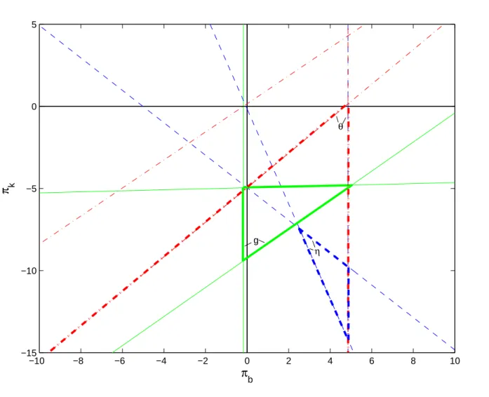
Alternatively, Example 3 varies Example 1 by allowing for a more substantial in-crease in savings through structural factors (by further loweringαand by raising the savings rate via a higher value of β) as well as policy-related factors (by considering a tax-transfer system which shifts the tax burden more strongly to second period income). In sum, this leads to a substantially higher steady-state debt ratio of0.14. Example 3: Consider Example 1, but let now α = 0.15 and β = 1 (i.e. sw =

β/(φ+β) = 1/2). Moreover, η = 0.74, θ =₋6.63, g = 3.47. Assuming b= 0, one obtains R= 0.32<1 +n= 2.43.At the golden rule steady state,R= 1 +n= 2.43,

yielding bgr = 2.11 > 0, k = 0.89, y = 14.74 and a debt ratio of bgr/y = 0.14.

Moreover, g/y = 0.24, η/y= 0.05, θ/y =₋0.45,i.e. the tax burden of agents in the second period is now substantially higher than in the first.

Figure 3 illustrates the stability regions associated with all three instruments for Example 3. The key result to be inferred from Figure 3 says that at sufficiently high debt level the three instrument-specific stability regions may no longer have a common intersection.21 _{More specifically, for the particular functional forms and}

baseline parameter values used in Example 3 the two stability regions associated with variations in gt and ηt cease to have a common intersection as bgr exceeds

some threshold value.22 _{This finding reflects that the high interest rate effect on}

20_{However, as far as the region associated with variations in g}

t is concerned, there is one

im-portant difference with Figure 1c. Since the interest rate effect on debt is now a key margin of

instability, stabilization in Figure 2can always be achieved if the primary surplus exclusively

re-acts to the capital stock imbalance, i.e. ifπb = 0local stability is always ensured for some values

πk<0. By contrast, if the primary surplus exclusively reacts to the debt imbalance (i.e. ifπk= 0)

stabilization can only be achieved if debt is low (like in Example 2).This holds no longer true in a

high debt regime (Example 3), indicating the implementability problems if debt is high.

21_{When interpreting the parameter values related to the effective savings rate in Examples1−3}

one should recall that the model set-up, counterfactually, does not allow for bequest motives.

Hence, in every period all assets need to be refinanced out of the savings of young agents.

22_{The fact that in Figure 3one side of the the η-triangle (corresponding to p(}

−1)_|η = 0) falls exactly onto a demarcation line of theθ-type stability region (corresponding to p(₋1)_|θ= 0) is not

generic but caused by the particular numerical assumption β = 1 (i.e. sw = 1), as one can verify

debt requires a stabilizing response via πk which leads to quite different

accumula-tion equaaccumula-tions under the gt-regime and theηt-regime. For an intuitive explanation,

it helps to realize that, compared with Figure 2, the stability triangle associated with the η_t-regime in Figure 3 has shifted to the southeast of the stability triangle associated with the gt-regime. Under the gt-regime points to the southeast of the

gt-triangle have one unstable eigenvalue. For the sake of the argument consider an

initial constellation with b0 > bgr and k0 < k. Then, under the gt-regime for

feed-back coefficients to the southeast of the gt-triangle there is, for given savings, too

much stabilization of debt dynamics, i.e. there is too little emission of new bonds

bt+1.This implies that the composition of next period’s assets(kt+1+bt+1)becomes

too productive, relative to the capacity of the economy to absorb investments in capital. However, points to the southeast of the gt-triangle may nevertheless be

consistent with fully stabilizing dynamics under the η_t-regime. The reason for this is that under the η_t-regime total savings will be lower because of the tax burden imposed on young agents. Because of this there is less scope that a strong reduction of bt+1 can trigger ‘overinvestment’ in physical capital kt+1. This reasoning shows

that the instrument-specific reactions to imbalances may not only be different, but also mutually exclusive if one wishes to maintain over time the knife-edge portfo-lio composition between government bonds and physical capital at the golden rule steady state.

If one attempts to make the role of the steady-state level of debt in Proposition 3 more precise one faces the challenge that bgr,in general, is a function of both

struc-tural and policy parameters. In the simple example economy introduced above, the sets corresponding to these two types of parameters amount to S ={α, β, φ, n, z, δ} and P ={η, θ, g}. From a policy perspective, it seems preferable to isolate imple-mentability problems which can be cured by policy changes. To control for this aspect requires to keep the structural parameters fixed and to look only at those variations in bgr which are policy-induced. For any set S consistent with the

ex-istence of a golden rule steady state it is possible to increase steady-state debt by shifting the tax burden more strongly to second period income. Yet, the maximum amount of debt that can be achieved with such a policy experiment depends itself onSand this debt level may not always be high enough to prevent the existence of a debt targeting rule which ensures implementability under all three instruments. This non-trivial interaction between structural and policy parameters is acknowledged in Proposition 4. A fairly tractable discussion of this interaction can be achieved by variations of the example economy, as shown in Appendix 1. Hence, to make the role of bgr in Proposition3more operational, Proposition 4draws directly on properties

of the example economy.

slopes downward. Conversely, if β > 1, p(₋1)_|η = 0 slopes downward and p(₋1)_|θ = 0 slopes

Proposition 4 Consider the example economy discussed in examples 1₋3, char-acterized by F(K, L) =zKα_L1−α _{and U(c, d) =φlnc+βlnd. Then, at any golden}

rule steady state the per capita debt level bgr >0 is a function of both structural

pa-rameters S ={α, β, φ, n, z, δ} and policy parameters P ={η, θ, g}. Consider golden

rule steady states which are characterized by the same set S, but different

policy-induced debt levels bgr because of differences in the setP. Then, many (although not

all conceivable) sets of S have the property that the debt targeting rule cannot be

implemented under all three instruments if bgr exceeds some policy-induced threshold

value b∗ gr >0.

Proof: For a proof of Propositions 3and 4, see Appendix 1.

4

Extensions

4.1

Alternative representations of the debt targeting rule

It is worth pointing out that there exist alternative representations of the debt targeting rule which lead to the same results summarized in Propositions 1₋4.We consider two particularly intuitive alternatives. As a starting point, we repeat the

flow budget constraint of the government

(1 +n)_·bt+1 =R(kt)·bt−πt,

and maintain the assumption that at the steady states under consideration the primary balance is zero, i.e. πt = 0.

First, let us assume that the debt targeting rule is now expressed in terms of stabi-lizing reactions of the overall deficit ∆t (i.e. inclusive interest payments), using

(1 +n)_·bt+1 = bt+∆t,

∆t = ∆(kt, bt) = (R(kt)−1)·bt−πt

Note that the deficit ∆t, at any moment in time, consists of a predetermined

com-ponent linked to interest payments on debt, and a policy comcom-ponent linked to the primary balance. Only the latter part can actively react to the two predetermined states of the economy, bt andkt.Accordingly, a debt targeting rule with stabilizing

reactions of the deficit to the states of the economy, in linearized form, needs to be established from

(1 +n)_·dbt+1 = ∆k·dkt+ (1 +∆b)·dbt, (28)

Consider the three linearized dynamic systems (18)-(19), (22)-(23), and (26)-(27) which were derived above for the three instruments. Using (28) as the second equa-tion in these 3 systems and replacing πk and πb by the terms R0(k)·b−∆k and

R(k)₋1₋∆b in thefirst equation of the 3systems, respectively, these systems can

be transformed into three new systems, all exhibiting two-dimensional dynamics in

kt and bt. However, since R(k), R0(k), and b are all evaluated at constant

steady-state values, the switch from the representation inπb−πk−space to a representation

in ∆b−∆k−space amounts to an affine transformation, which leaves the results of

Propositions 1₋4unaffected.

Second, the debt targeting rule can be reinterpreted as a rule which expresses the issuance of new per capita debt directly in terms of stabilizing reactions to the states of the economy, according to

(1 +n)_·bt+1 = ht, (30)

ht = h(kt, bt) =R(kt)·bt−πt.

After linearizing (30) and substituting out the relevant terms in the three systems, it is clear that a switch from a representation inπb−πk−space to a representation in

hb−hk−space amounts to another affine transformation, leaving, again, the results

of Propositions 1₋4unaffected.

4.2

Endogenous labour supply and distortionary taxes

The purpose of this subsection is to show that all the central findings of Section 3, as summarized by Propositions 1₋4, prevail qualitatively in a richer setting which is characterized by an endogenous labour supply and distortionary taxes. Yet, there is an interesting twist to the results of this richer setting which is worth pointing out. To this end, we assume now that preferences are described by the more general expression

U(ct−ϕ(lt), dt+1),

where lt denotes the variable labour supply of the representative young agent and

the function ϕ(lt) captures the disutility of work, with ϕ(0) > 0, and ϕ0(lt) > 0,

ϕ00_(l

t)>0for alllt >0.As discussed in Greenwood et al. (1988), this labour supply

specification has the convenient feature that it can be solved independently from the intertemporal consumption and savings decisions, allowing for easy comparability with the analysis of the previous section. Moreover, also for simple comparability, it is assumed that total tax revenues have a lump-sum and a distortionary component

η_t=η+τtwtlt, (31)

whereτtdenotes the wage income tax rate. We maintain the assumption that for the

matter. In contrast to the previous analysis, however, the entire out-of-steady-state adjustment burden falls on variations of the distortionary component τt, whenever

tax adjustments are the preferred instrument to stabilize the debt level around the steady-state target. Accordingly, the objective can be replaced by

U(wtlt−ϕ(lt)−ηt−st, Rt+1st+θt+1),

giving rise to the pair of first order conditions

ϕ0(lt) = (1−τt)wt (32)

U1 = Rt+1U2. (33)

With an endogenous labour supply, the labour market equilibrium condition be-comes Lt =ltNtand thefirst-order conditions from the profit maximization offirms

are given by

Rt = 1−δ+FK(kt, lt) (34)

wt = FL(kt, lt). (35)

Combining (31), (32), and (35) yields

ltϕ0(lt) =ltFL(kt, lt)−(ηt−η),

which implicitly defines the equilibrium labour supply

lt =l(kt, ηt)

in the vicinity of some steady state l = l(k, η), with partial derivatives lk(k, η) = FLK(k,l)

ϕ00(l)−FLL(k,l) > 0 and lη(k, η) =

−1

l·[ϕ00(l)−FLL(k,l)] < 0.

23 _{To keep the structure of the}

analysis as similar as possible to Section2, we define the adjusted gross wage income net of the disutility term ϕ(lt) as

e

wt≡wtlt−ϕ(lt) =FL(kt, lt)·lt−ϕ(lt) =we(kt, ηt). (36)

Using (36), the savings function reduces to

st=s(wet−ηt+ θt+1 Rt+1 , Rt+1)− θt+1 Rt+1 .

23_{For clarification, note that partial derivatives use the notation l}

k(k, η) = _{δ kt}δ lt ¯ ¯ ¯_kt=k and lη(k, η) = _{δ η}δ lt t ¯ ¯ ¯ ηt=η

, i.e. in the latter case the derivative is taken with respect to η_t and then