Doctoral Dissertations Graduate School
Fall 2012
Adaptive grid based localized learning for
multidimensional data
Sheetal Saini
Follow this and additional works at:https://digitalcommons.latech.edu/dissertations
ADAPTIVE GRID BASED LOCALIZED LEARNING FOR MULTIDIMENSIONAL DATA
by
Sheetal Saini, B. Eng.
A Dissertation Presented in Partial Fulfillment of the Requirements of the Degree
Doctor of Philosophy
COLLEGE OF ENGINEERING AND SCIENCE LOUISIANA TECH UNIVERSITY
All rights reserved
INFORMATION TO ALL USERS
The quality of this reproduction is dependent upon the quality of the copy submitted. In the unlikely event that the author did not send a complete manuscript
and there are missing pages, these will be noted. Also, if material had to be removed, a note will indicate the deletion.
UMI 3534292
Published by ProQuest LLC 2012. Copyright in the Dissertation held by the Author. Microform Edition © ProQuest LLC.
All rights reserved. This work is protected against unauthorized copying under Title 17, United States Code.
ProQuest LLC
789 East Eisenhower Parkway P.O. Box 1346
LOUISIANA TECH UNIVERSITY
by_ entitled
THE GRADUATE SCHOOL
9/21/2012 Date
We hereby recommend that the dissertation prepared under our supervision
Sheetal Saini
Adaptive Grid Based Localized Learning for Multidimensional Data
be accepted in partial fulfillment of the requirements for the Degree of
Doctor of Philosophy in Computational Analysis and Modeling
Supervisor oQ)issctiation Research Head ofDepartment
Computational Analysis and Modeling
Department Recommendation concurred in:
yfijmj W TKrmjtJon/ S-P
Apprised: C J
Director of Graduate Studies
—
/ [ I
Dean of the College
Advisory Committee
Approved:
Dean of tfte Graduate School
CiS I orm 13a (6/07)
Rapid advances in data-rich domains of science, technology, and business has amplified the computational challenges of "Big Data" synthesis necessary to slow the widening gap between the rate at which the data is being collected and analyzed for knowledge. This has led to the renewed need for efficient and accurate algorithms, framework, and algorithmic mechanisms essential for knowledge discovery, especially in the domains of clustering, classification, dimensionality reduction, feature ranking, and feature selection. However, data mining algorithms are frequently challenged by the sparseness due to the high dimensionality of the datasets in such domains which is particularly detrimental to the performance of unsupervised learning algorithms.
The motivation for the research presented in this dissertation is to develop novel data mining algorithms to address the challenges of high dimensionality, sparseness and large volumes of datasets by using a unique grid-based localized learning paradigm for data movement clustering and classification schema. The grid-based learning is
recognized in data mining as these algorithms are inherently efficient since they reduce the search space by partitioning the feature space into effective partitions. However, these approaches have not been successfully devised for supervised learning algorithms or sparseness reduction algorithm as they require careful estimation of grid sizes, partitions and data movement error calculations. Grid-based localized learning algorithms can scale well with an increase in dimensionality and the size of the datasets.
iv
To fulfill the goal of designing and developing learning algorithms that can handle data sparseness, high data dimensionality, and large size of data, in a concurrent manner to avoid the feature selection biases, a set of novel data mining algorithms using grid-based localized learning principles are developed and presented. The first algorithm is a unique computational framework for feature ranking that employs adaptive grid-based data shrinking for feature ranking. This method addresses the limitations of existing feature ranking methods by using a scoring function that discovers and exploits dependencies from all the features in the data. Data shrinking principles are established and metricized to capture and exploit dependencies between features. The second core algorithmic contribution is a novel supervised learning algorithm that utilizes grid-based localized learning to build a nonparametric classification model. In this classification model, feature space is divided using uniform/non-uniform partitions and data space subdivision is performed using a grid structure which is then used to build a classification model using grid-based nearest-neighbor learning. The third algorithm is an unsupervised clustering algorithm that is augmented with data shrinking to enhance the clustering performance of the algorithm. This algorithm addresses the limitations of the existing grid-based data shrinking and clustering algorithms by using an adaptive grid-based learning. Multiple experiments on a diversified set of datasets evaluate and discuss the effectiveness of dimensionality reduction, feature selection, unsupervised and supervised learning, and the scalability of the proposed methods compared to the established
The author grants to the Prescott Memorial Library of Louisiana Tech University the right to reproduce, by appropriate methods, upon request, any or all portions of this Dissertation. It is understood that "proper request" consists of the agreement, on the part of the requesting party, that said reproduction is for his personal use and that subsequent reproduction will not occur without written approval of the author of this Dissertation. Further, any portions of the Dissertation used in books, papers, and other works must be appropriately referenced to this Dissertation.
Finally, the author of this Dissertation reserves the right to publish freely, in the literature, at any time, any or all portions of this Dissertation.
Author _ SHEETAL SAINI
Date 09/21/2012
GS Form 14 (5/03)
DEDICATION
To my family and elders for their sacrifices, support, patience, and endless prayers for me.
ABSTRACT iii
DEDICATION vi
LIST OF TABLES xii
LIST OF FIGURES xiv
ACKNOWLEDGEMENTS xvii
CHAPTER 1 INTRODUCTION 1
1.1 Knowledge Discovery in Databases 2
1.2 Data Mining 4 1.3 Learning Techniques 5 1.3.1 Unsupervised Learning 6 1.3.2 Supervised Learning 6 1.4 Localized Learning 7 1.4.1 Nearest-Neighbor Learning 7
1.4.2 Grid-Based Nearest-Neighbor Learning 8
1.5 Dissertation Organization 9
CHAPTER 2 RELATED RESEARCH 12
2.1 Grid-Based Localized Learning 13
2.2 Data Shrinking 14
2.2.1 Point-Based Approach 16
2.2.2 Grid-Based Approach 16
2.3 Feature Selection and Ranking 16 2.4 Classification 17 2.5 Clustering 19 2.5.1 Partitioning-Based Clustering 19 2.5.2 Density-Based Clustering 19 2.5.3 Hierarchical Clustering 20
2.5.3.1 Agglomerative Hierarchical Clustering 20
2.5.3.2 Divisive Hierarchical Clustering 21
2.5.4 Grid-Based Clustering 21
2.5.4.1 Uniform Grid-Based Clustering 22
2.5.4.2 Non-Uniform Grid-Based Clustering 22
2.5.5 Data Shrinking Based Clustering 22
2.6 Conclusion 24
CHAPTER 3 PRELIMINARIES OF GRID-BASED LOCALIZED LEARNING 25
3.1 Notations 25
3.2 Formal Definitions 26
CHAPTER 4 GRID-BASED LOCALIZED LEARNING FOR DATA
PREPROCESSING 35
4.1 Data Preprocessing 36
4.2 Data Sparseness 38
4.3 Research Motivation 39
4.3.1 Limitations of Existing Techniques 39
4.3.2 Advantages of Non-Uniform Grid 40
4.4.1 Datasets 41
4.4.2 Effect of Sparseness 42
4.4.3 Comparative Study 43
4.4.3.1 Comparison of Partitioning Methods 43
4.4.3.2 Comparison of Shrinking Methods 46
4.5 Conclusion 50
CHAPTER 5 GRID-BASED LOCALIZED LEARNING FOR FEATURE
RANKING 51
5.1 Research Motivation 52
5.2 Problem Statement 53
5.3 Methodology 53
5.3.1 Data Preprocessing 54
5.3.2 Adaptive Grid Generation 54
5.3.3 Data Shrinking 55
5.3.3.1 Data Movement Model 56
5.3.3.2 Data Shrinking Process 57
5.3.4 Feature Ranking Method 58
5.4 Results and Discussions 60
5.4.1 Datasets 60
5.4.2 Validation 61
5.4.3 Experiments 61
5.5 Conclusion 68
CHAPTER 6 GRID-BASED LOCALIZED LEARNING FOR CLASSIFICATION 69
X
6.2 Problem Statement 70
6.3 Methodology 70
6.3.1 Data Preprocessing 71
6.3.2 Grid Generation 71
6.3.2.1 Uniform Grid Generation 71
6.3.2.2 Adaptive Grid Generation 72
6.3.3 Training Phase 74
6.3.4 Test Phase 76
6.4 Results and Discussions 77
6.4.1 Datasets 78
6.4.2 Validation 79
6.4.3 Experiments 80
6.4.3.1 Scalability Analysis 80
6.4.3.2 Comparative Analysis 87
6.4.4 Time Complexity Analysis 89
6.5 Conclusion 90
CHAPTER 7 GRID-BASED LOCALIZED LEARNING FOR CLUSTERING 92
7.1 Research Motivation 93
7.2 Problem Statement 93
7.3 Methodology 94
7.3.1 Data Preprocessing 95
7.3.2 Adaptive Grid Generation 95
7.3.2.2 Data Transformation 97
7.3.2.3 MOSAH Partitioning 98
7.3.2.4 Algorithmic Description 99
7.3.3 Adaptive Grid-Based Shrinking 100
7.3.3.1 Ranking Neighboring Grid Cells 100
7.3.3.2 Data Movement Model 102
7.3.3.3 Data Shrinking Process 103
7.3.4 Adaptive Grid-Based Clustering 105
7.4 Results and Discussion 107
7.4.1 Datasets 107
7.4.2 Validation 108
7.4.3 Experiments 109
7.4.3.1 Scalability Analysis 110
7.4.3.2 Comparative Analysis 114
7.4.4 Time Complexity Analysis 129
7.5 Conclusion 130
CHAPTER 8 CONCLUSIONS 132
8.1 Contribution to Grid-Based Supervised Learning 132 8.2 Contribution to Grid-Based Unsupervised Learning 133
LIST OF TABLES
Table 5.1: Common Top Ranked Features 63
Table 5.2: Comparison of F-measure for Neural Network 64
Table 5.3: Comparison of F-measure for PART 65
Table 5.4: Comparison of F-measure for Logistic Regression 66 Table 5.5: Comparison of Avg. Precision, Recall, Accuracy for PART 66 Table 5.6: Comparison of Avg. Precision, Recall, Accuracy for Logistic Regression... 67 Table 5.7: Comparison of Avg. Precision, Recall, Accuracy for Neural Network 68 Table 7.1: Benchmark v/s Adaptive Shrinking Based Method on Wine Dataset 115 Table 7.2: CURE v/s Adaptive Shrinking Based Method on Wine Dataset 116 Table 7.3: DBSCAN v/s Adaptive Shrinking Based Method on Wine Dataset 116 Table 7.4: Benchmark v/s Adaptive Shrinking Based Method on Ecoli Dataset 117 Table 7.5: CURE v/s Adaptive Shrinking Based Method on Ecoli Dataset 118 Table 7.6: DBSCAN v/s Adaptive Shrinking Based Method on Ecoli Dataset 119 Table 7.7: Benchmark v/s Adaptive Shrinking Based Method on Protein Dataset 120 Table 7.8: CURE v/s Adaptive Shrinking Based Method on Protein Dataset 121 Table 7.9: DBSCAN v/s Adaptive Shrinking Based Method on Protein Dataset 122 Table 7.10: Benchmark Method v/s Adaptive Shrinking Based Method on a
Synthetic Dataset 123
Table 7.11: CURE v/s Adaptive Shrinking Based Method on a Synthetic Dataset 124 Table 7.12: DBSCAN v/s Adaptive Shrinking Based Method on a Synthetic
Dataset 124
Table 7.13: Benchmark Method v/s Adaptive Shrinking Based Method on a
Synthetic Dataset 125
Table 7.14: CURE v/s Adaptive Shrinking Based Method on a Synthetic Dataset 126 Table 7.15: DBSCAN v/s Adaptive Shrinking Based Method on a Synthetic
Dataset 127
Table 7.16: Benchmark Method v/s Adaptive Shrinking Based Method on a
Synthetic Dataset 128
Table 7.17: CURE v/s Adaptive Shrinking Based Method on a Synthetic Dataset 129 Table 7.18: DBSCAN v/s Adaptive Shrinking Based Method on a Synthetic
LIST OF FIGURES
Figure 1.1: KDD Process 3
Figure 1.2: Data Mining as Confluence of Multiple Disciplines 5
Figure 1.3: Two-Dimensional Grid 8
Figure 1.4: Key Elements of This Dissertation 9
Figure 2.1: Grid-Based Localized Learning Paradigm 14
Figure 2.2: Data Shrinking Approaches 15
Figure 2.3: Types of Data Grids 22
Figure 3.1: A Two-Dimensional Uniform Grid 27
Figure 3.2: A Two-Dimensional Non-Uniform Grid 28
Figure 3.3: A Grid Cell Representation 28
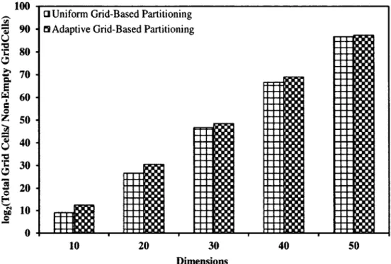
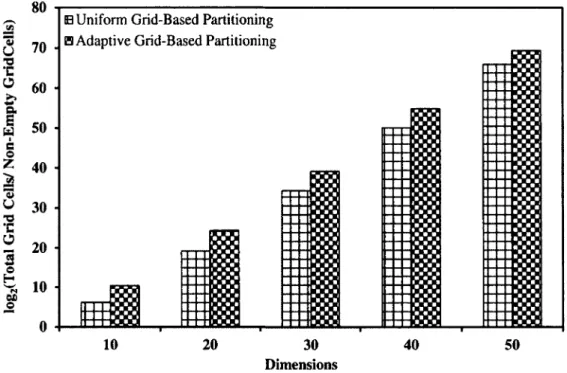
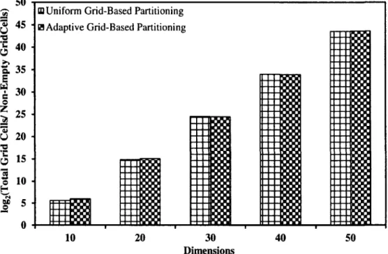
Figure 4.1: Average Pairwise Euclidean Distance v/s Dimensions 42 Figure 4.2: log2 (Total Grid Cells/Non-Empty Grid Cells) v/s Dimensions 44 Figure 4.3: log2 (Total Grid Cells /Non-Empty Grid Cells) v/s Dimensions 45 Figure 4.4: log2 (Total Grid Cells/Non-Empty Grid Cells) v/s Dimensions 46 Figure 4.5: Cumulative Wavelet Entropy v/s Dimensions 47
Figure 4.6: Cumulative Energy v/s Dimensions 48
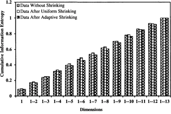
Figure 4.7: Cumulative Information Entropy v/s Dimensions 49
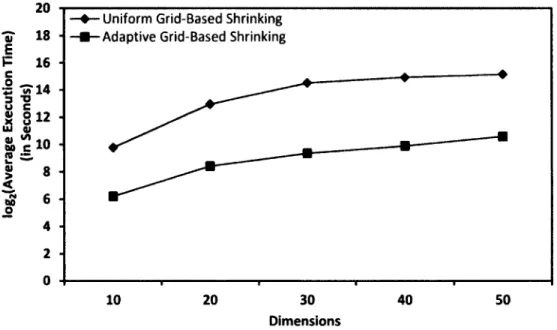
Figure 4.8: Average Execution Time v/s Dimensions 50
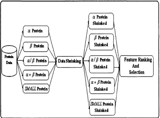
Figure 5.1: Data Shrinking Based Feature Ranking Framework 54
Figure 5.2: Adaptive Grid Generation Algorithm 55
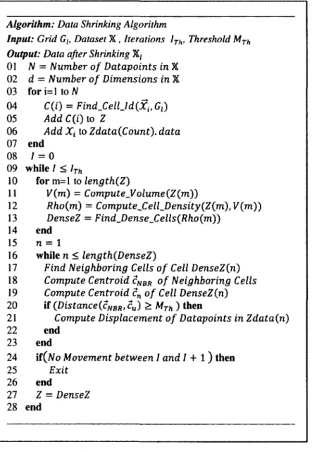
Figure 5.3: Adaptive Data Shrinking Algorithm 57 Figure 5.4: Feature Ranking and Selection Algorithm 59
Figure 5.5: Comparison of Top Ranked Features 62
Figure 6.1: Variance-Based Partitioning Algorithm 73
Figure 6.2: Training Phase of the Grid-Based Classifier 75 Figure 6.3: Test Phase of the Grid-Based Classifier 77 Figure 6.4: Training Phase Execution Time v/s Dimensions 81 Figure 6.5: Training Phase Execution Time v/s Dataset Size 82 Figure 6.6: Average Execution Time/Sample v/s Dimensions 83 Figure 6.7: Average Execution Time/Sample v/s Dataset Size 83
Figure 6.8: Execution Time v/s Dimensions 84
Figure 6.9: Execution Time v/s Dataset Size 85
Figure 6.10: Average Execution Time/Sample v/s Dimensions 86 Figure 6.11: Average Execution Time/Sample v/s Dataset Size 86 Figure 6.12: Comparative Study on Letter Recognition Dataset 87 Figure 6.13: Comparative Study on Profile Correlation Feature Set 88 Figure 6.14: Comparative Study on Protein Structural Classification Dataset 89 Figure 7.1: Adaptive Shrinking Based Clustering Approach 94 Figure 7.2: MOSAH Partitioning of Micro-partitions 98 Figure 7.3: Data Adaptive Grid Generation Algorithm 99 Figure 7.4: A Two-Dimensional Grid with Cell ID's 101 Figure 7.5: Hierarchical Decomposition of Data Adaptive Partitions 103 Figure 7.6: Pseudo-code for Data Shrinking Algorithm 104
xvi
Figure 7.7: Grid-Based Hierarchical Clustering 105
Figure 7.8: Pseudo-code for Adaptive Grid-Based Clustering 106 Figure 7.9: Execution Time v/s Dataset Size (Analysis for Grid Generation
Method) 110
Figure 7.10: Execution Time v/s Dimensions (Analysis for Grid Generation
Method) Ill
Figure 7.11: Execution Time v/s Dataset Size (Analysis for Data Shrinking
Method) 112
Figure 7.12: Execution Time v/s Dimensions (Analysis for Data Shrinking
Method) 112
Figure 7.13: Execution Time v/s Dataset Size (Analysis for Clustering Method) 113 Figure 7.14: Execution Time v/s Dimensions (Analysis for Clustering Method) 113
My dissertation has not only tested my skills and determination, but it has also tested the support and patience of my family, close friends and people around me. First of all, I would like to thank Dr. Sumeet Dua for providing his guidance and financial
support throughout my PhD. I am grateful to the Louisiana Biomedical Research
Network (LBRN), the Louisiana Alliance for Simulation-Guided Materials Applications (LA-SiGMA), National Science Foundation (NSF), and National Institutes of Health (NIH) for providing financial support for my education and research. I am only able to achieve my goals through the support and patience of my whole family. I am indebted to them for their support and patience throughout my PhD, especially my grandmother's and my mother's endless prayers for me. Finally, I would like to thank my close friends who extended their valuable support whenever possible. I would have not finished it without their support.
CHAPTER 1
INTRODUCTION
The common characteristics of contemporary datasets are multi dimensionality, sparseness, and the large size of the data. These characteristics are the main motivation behind the development of novel algorithms and frameworks for automated and
sophisticated data mining systems that search nontrivial, previously unknown, and potentially useful knowledge from the data. Many researchers and scientists have developed automated systems that address these problems. As a result, ample literature on these problems and potential solutions are available. However, there is always a need to improve the existing algorithms, frameworks, and systems to achieve better
performance and address the shortcomings of the existing data mining techniques. Data mining techniques are commonly categorized based on the type of knowledge mined by these techniques. The most common data mining techniques are classification, and clustering. Classification is used to build models based on the data and known class labels that can describe data classes or groups [1, 2]. It predicts categorical class labels based on known examples. Therefore, it is also referred to as supervised learning. There are ample classification techniques, such as decision tree classifier, Bayesian classifier, rule based classifier, neural network classifier, support vector machine, k-nearest-neighbor classifier, and others. Unlike classification, clustering and unsupervised learning does not rely on predefined classes and class-labeled training
examples. For this reason, clustering is a form of learning by observation, rather than learning by examples.
The algorithms presented in this dissertation are created using the grid-based localized learning paradigm of data mining for knowledge discovery. To explain these paradigms, the understanding of the knowledge discovery process, data mining, machine learning, and localized learning are critical. Therefore, the process of knowledge
discovery in databases (KDD), data mining, which is the core of the KDD process, machine learning, and localized learning and grid-based localized learning paradigms are outlined and explained in this chapter.
1.1 Knowledge Discovery in Databases
The phrase knowledge discovery in databases commonly (KDD) refers to the process of extracting nontrivial, implicit, previously unknown, valid, potentially useful, and understandable patterns/knowledge from data in databases by applying data mining algorithms [1]. Knowledge discovery in databases (KDD) is an interactive and iterative process that involves many decisions made by the end user. Knowledge discovery in databases process includes data selection, data preprocessing, data transformation, data mining, and data evaluation/interpretation. All the steps involved in the KDD process are defined and discussed below. Figure 1.1 depicts the KDD process.
3 Data Evaluation/ Interpretation Data Mining Data T ransf ormation Patterns Data Preprocessing Data Selection Target Data >,D»ta Figure 1.1: KDD Process
1. Data Selection: Data selection is the process of creating a target dataset on which knowledge discovery is to be performed. Extracting a target dataset refers to the selection of a subset of data attributes, data samples, or both attributes and samples that are relevant for the analysis task at hand [1].
2. Data Preprocessing: Data preprocessing is a data cleaning process, which involves operations such as removing noise, filling in missing values, and eliminating inconsistent data. It requires identification and selection of appropriate method for each operation.
3. Data Transformation: Data transformation is the process of converting data into the format that is most appropriate for relevant data mining tasks. Data
transformation includes data aggregation, data smoothing, data normalization, data generalization, and feature construction [1].
4. Data Mining: Data mining in the KDD process is a step that involves
extracting patterns/knowledge of interest in a particular representational form by applying an appropriate data modeling technique. These data modeling techniques include
association rule discovery, classification models, clustering models, and prediction models [1].
5. Data Evaluation/Interpretation: Data evaluation and interpretation is the process in which discovered patterns/knowledge is evaluated. This step also involves the interpretation of patterns through visualization or other means of representation.
1.2 Data Mining
Data mining is the process of extracting or mining interesting and useful patterns or knowledge from the given data [2]. In data mining, the term 'extraction of patterns or knowledge' refers to fitting a model to data, finding implicit structure from the data, or describing the data through a high level of abstraction [3]. There are two prevalent perspectives regarding data mining. The first perspective treats data mining as a synonym for knowledge discovery in databases (KDD), and the second perspective treats data mining as an essential step in the process of knowledge discovery in databases (see Figure 1.1). In both cases, data mining is an interdisciplinary field, and it is a confluence of multiple disciplines. Disciplines that contribute to data mining are database systems, statistics, machine learning, visualization, and information science [2]. It relies heavily on machine learning, pattern recognition, mathematics, and statistical techniques to find
5
patterns/knowledge from data [2], Figure 1.2 depicts the interdisciplinary view of data mining.
Figure 1.2: Data Mining as Confluence of Multiple Disciplines
As shown in Figure 1.2, data mining is the process of applying specific methods to extract interesting patterns/knowledge from the data [1].
1.3 Learning Techniques
Machine learning is a domain of artificial intelligence methods that are designed to automatically learn to recognize the evolving behavior of the system based on sample data. The term also refers to designing algorithms that optimize the performance criteria of the chosen mathematical model based on the input data [4]. These mathematical models can be predictive or descriptive. Predictive models are used to predict future outcomes, and descriptive models are used to gain knowledge about the data. Machine learning techniques can be broadly categorized into supervised learning and unsupervised
learning [4J. In subsections 1.3.1 and 1.3.2, supervised learning and unsupervised learning methods are explained.
1.3.1 Unsupervised Learning
Unsupervised learning is learning by observation, rather than learning by
example. It does not rely on predefined classes and class-labeled training examples [2]. In unsupervised learning, the class label of each data point is not known. In some cases, the total number of classes to be learned may not be known in advance. The aim of the unsupervised learning is to identify patterns in the data that occur more often than others based on the structure of the data space [4, 5]. Commonly employed unsupervised learning techniques are clustering, subspace clustering, bi-clustering, and density estimation. The basic principle of all these techniques is to group the data into clusters such that data points within a cluster are very similar to each other but are very dissimilar to the data points in other clusters.
1.3.2 Supervised Learning
Supervised learning is learning by example. It relies on the knowledge about the class labels of each data point and the number of classes. Supervised learning is a two-step process. In the first two-step, a learning model is built using the predefined number of classes and class labels of each data point. This learning step is called the training phase. Each data point is assumed to belong to a predefined class which is determined by a class label attribute. The class label attribute is categorical, and each value serves as a class identifier [2]. The data points that are part of the training phase are collectively referred to as a training set and are selected from the given dataset. In the second step, the model learned in the first step is used to assign class labels to the data points that do not have any class label. This step is also called the testing phase. The data points that are part of
7
the testing phase are collectively referred to as the test set and are also selected from the given dataset for validation.
1.4 Localized Learning
Two commonly used learning techniques are known as parametric learning and nonparametric learning, respectively [4]. In parametric learning, a valid model is assumed for the whole input space, whereas in nonparametric learning no model is assumed. In nonparametric learning, there is no single global model, but local models are built based on the local neighborhood [4]. Therefore, a nonparametric learning strategy can also be referred to as 'localized learning.'
All the localized learning methods follow the same philosophy and can only be differentiated based on the similarity criteria of the neighborhood. Distance based nearest-neighbor learning is the most common form of neighborhood learning, but other methods such as grid-based nearest-neighbor learning and rule based nearest-neighbor learning are used in machine learning as well [2, 6, 7, 8, 9, 10]. Localized learning refers to the method of learning in which local models are learned or built based on a local neighborhood.
1.4.1 Nearest-Neighbor Learning
Nearest-neighbor learning is based on the intuition that an input data instance is more likely to be similar to input data instances that are in the neighborhood. 1-NN and k-NN are two common neighbor learning strategies. In the 1-NN neighbor method only one neighbor is identified, whereas, in the k-NN nearest-neighbor method the total 'k' numbers of nearest-nearest-neighbors are identified [5]. Nearest-neighbor learning is also referred to as a prototype method [5]. Nearest-Nearest-neighbor learning
has been used for both supervised (k-NN classifier) and unsupervised (k-NN estimator) learning. Grid-based nearest-neighbor learning, an important aspect of the research presented in the first part of the dissertation, is explained below.
1.4.2 Grid-Based Nearest -Neighbor Learning
The idea of grid-based nearest-neighbor learning originates from a class of
clustering algorithms known as grid-based clustering algorithms [6,7, 8, 9,10, 11, 12]. In grid-based clustering algorithms, initially, dimensions are divided into two or more partitions, and a grid structure is imposed on the feature space. This grid structure then divides the feature space into small cells called grid cells (see Figure 1.3). Next, each data sample is mapped onto the grid structure and assigned to a corresponding grid cell.
Finally, these grid cells are used for clustering, and neighbors are identified by searching for adjacent non-empty grid cells. Figure 1.3 depicts a two-dimensional grid structure.
Neighbors Non-Empty Cell
Grid Structure fS a •2 o <£ «n § o E
5
<n <N o Grid Cells Data Point 0.0 0.25 0.50 0.75 1 Dimension 19
Thus, in grid-based nearest-neighbor learning, the definition of a neighborhood is based on the concept of grid cells, rather than individual data points.
1.5 Dissertation Organization
The remainder of the dissertation is further divided into seven more chapters. The organization and the outline of the remaining dissertation are as follows. A pictorial representation of the key elements of this dissertation is presented in Figure 1.4.
DlsVI l< I \1 ION
Figure 1.4: Key Elements of This Dissertation
Chapter 2: In Chapter 2, research related to the problem domain of this dissertation is presented. It includes discussion on pertinent literature review on data shrinking preprocessing, feature ranking, classification and clustering techniques.
Chapter 3: In Chapter 3, preliminaries of grid-based localized learning are presented. It includes description of notations that are used in subsequent chapters. It also includes formal definitions of various terminologies that are essential in understanding the concepts of grid-based localized learning paradigm.
Chapter 4: In Chapter 4, the need for data preprocessing and various methods of data preprocessing techniques are discussed. However, special emphasis is given to data shrinking preprocessing techniques and its need for sparseness reduction in
multidimensional data. This chapter also includes experimental studies that demonstrate the benefits of the newly developed sparseness reduction technique presented in this dissertation.
Chapter 5: In Chapter 5, a feature ranking method is presented that uses the grid-based localized learning method. This chapter discusses research motivation, problem statement, and methodology. Experimental studies are also presented in which
comparative studies of the existing and newly developed feature ranking methods are performed.
Chapter 6: In Chapter 6, a grid-based localized learning method is presented for classification. This chapter includes discussion on research motivation, problem
statement and explains the developed grid-based classification framework. Finally, experimental studies are presented to compare the newly developed framework with existing methodology.
Chapter 7: In Chapter 7, grid-based data shrinking and clustering algorithm is presented. This chapter includes motivation and the problem statement for the research.
11
The developed methodology is also explained in detail which is further supported by experimental study conducted.
Chapter 8: In Chapter 8, the conclusions and future directions are presented. It also includes the outcomes of this dissertation.
RELATED RESEARCH
Many data mining algorithms have been developed to address the challenges of data sparseness, the curse of dimensionality, and the large size of the data [2,4, 5, 13, 14]. Many learning techniques have been developed to address these challenges. These learning techniques are categorized into parametric and nonparametric approaches [2,4, 5, 15, 16, 17, 18]. In parametric learning approaches, a global model is built for all data samples at once. In nonparametric learning approaches, local models are built using the local neighborhood [4, 5]. Therefore, nonparametric approaches can also be referred to as localized learning approaches. Nonparametric techniques of data modeling have
advantages over parametric techniques because of its simplicity [4, 5]. In the past, several approaches have been developed for data mining using both parametric and
nonparametric learning models [2,4, 5]. However, the focus of the research in this
dissertation is on using grid-based localized learning techniques to address the challenges of data sparseness, the curse of dimensionality, and the large size of data in data mining. This chapter includes a discussion on the research related to clustering techniques , feature ranking techniques, data shrinking techniques, and classification techniques to provide the general idea of these techniques and demonstrate a need to develop grid-based localized learning techniques in these areas to address data mining challenges.
13
The remainder of the chapter is organized as follows. In Section 2.1, grid-based localized learning is explained and discussed. In Section 2.2, research related to data shrinking preprocessing, including existing grid-based shrinking approaches and non-grid/point-based approaches, is explained [13,14, 20,21, 22, 23, 24]. In Section 2.3, research related to feature selection and ranking is discussed. In 2.4, research related to classification techniques. In Section 2.5, research related to clustering techniques is discussed in general. However, special emphasis is given to grid-based clustering techniques and clustering techniques that are augmented with data preprocessing techniques to boost their performance. Finally, in Section 2.6, the conclusions of this chapter are presented.
2.1 Grid-Based Localized Learning
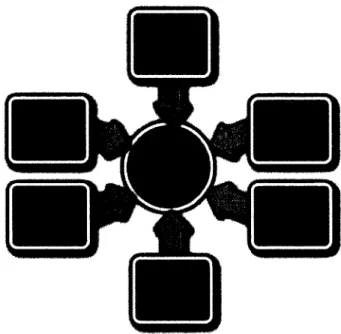
Grid-based learning algorithms are nonparametric learning algorithms. In these algorithms, a grid structure is imposed on the data space that divides it into smaller partitions called grid cells. Data is mapped in these grid cells which are then used to build local models using grid-based neighborhood learning [2]. In the past, grid-based localized learning has been used extensively for designing unsupervised learning algorithms such as clustering, subspace clustering, and data shrinking [25, 26, 27, 28, 29,13,14]. In this dissertation, the scope of based localized learning is further expanded into grid-based data preprocessing techniques, such as data shrinking, grid-grid-based supervised learning techniques, grid-based clustering techniques, and grid-based data shrinking and dimensionality reduction [30, 31]. Figure 2.1 depicts a schematic of a grid-based
Figure 2.1: Grid-Based Localized Learning Paradigm
The schematic depicts the applicability of gird-based localized learning in the area of clustering, classification, data shrinking and dimensionality reduction techniques.
2.2 Data Shrinking
Data shrinking is a data preprocessing technique that is used to reduce the sparseness in a multidimensional dataset. The sparseness of the data increases as the number of dimensions increases [13, 14]. As a result, clusters of data points lack distinct boundaries, and the detection of clusters with better accuracies is severely affected. The data shrinking process utilizes the inherent characteristics of data distribution and outputs a more condensed and reorganized dataset [13, 14]. In the data shrinking process, the movement of data points is performed through the principle of data gravitation. Points are attracted by their surrounding neighbors and move toward the center of their natural clusters along the direction of the density gradient [20, 21, 22, 23, 24], Furthermore, data shrinking approaches can be broadly categorized into grid-based approaches and
non-15
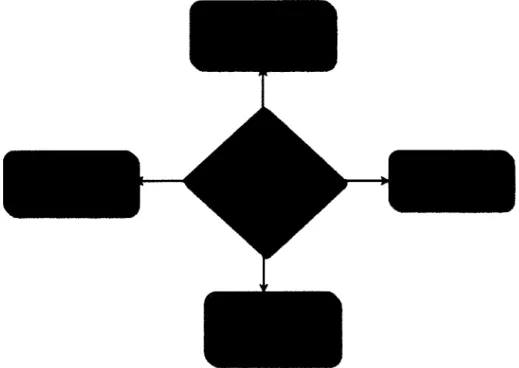
grid/point-based approaches. A pictorial representation of the categorization of data shrinking approaches is presented in Figure 2.2.
1. GRAVITATIONAL MODELS [20,21,22,23] 2. CLUES [24]
i r <jr
NON-UNIFORM GRID-BASED UNIFORM GRID-BASED GRAVITATIONAL MODEL GRAVITATIONAL
[PROPOSED] MODEL [13,14]
Figure 2.2: Data Shrinking Approaches
Grid-based data shrinking approaches employs grid-based partitioning to map the data in a grid structure. Initially, data is mapped on a grid structure and grid cell
corresponding to each data point identified, and data points that are occupied in the same grid cells are also identified. Data points in the same grid cell move to other locations as a single unit. The movement of data points in each grid cell is then performed using the principle of data gravitation [13, 14]. Non-grid-based data shrinking approaches use the principle of data gravitation on individual data points. In these approaches, each data point is moved by a simulated movement of data points [20, 21, 22, 23, 24], Grid-based approaches are faster, scalable, and computationally less expensive than non-grid/point-based approaches.
2.2.1 Point-Based Approach
In the past, many point-based data shrinking approaches have been used to employ the principle of data gravitation or gravitational transform [20, 21, 22, 23, 24]. The essence of all the approaches is as follows. Initially, a model of attraction (data gravitation) is assumed between the data points and a force of attraction is applied on a data point by its surrounding/neighboring data points. Then, this force of attraction enables the simulated movement of the data points. This process is applied for a specified number of iterations or until some stopping criterion is satisfied.
2.2.2 Grid-Based Approach
In the past only one grid-based data shrinking approach has been developed [13]. The overall process for this approach can be summarized as follows. Initially, multi-scale uniform grids are generated. Next, data points are mapped on the uniform grid structure and corresponding grid cells. Then, data points in each dense cell are moved toward the data centroid of the surrounding dense cells. This process is repeated until a specified movement threshold is achieved or for a specified number of iterations.
2.3 Feature Selection and Ranking
Feature selection is a process of identifying and selecting a subset of features from a given set of features to reduce the dimensionality of the data by optimizing an evaluation criterion. Feature selection reduces the dimensionality by removing irrelevant, noisy, and redundant features from the feature set [32, 33, 34, 35]. Application of feature selection as a preprocessing step in a data mining algorithm can greatly improve the accuracies and overall learning time of those algorithms. Feature selection techniques are essential and better techniques are always needed. Feature selection is frequently used in
17
data mining, especially in the fields of Bioinformatics, web mining, and other high dimensional data domains. The datasets in these domains may contain features that are irrelevant and unimportant and may have no predictive power. In fact, for some
problems, only a small subset of features is usually relevant.
Feature selection techniques can be categorized into two categories, the filter model or the wrapper model [36, 37, 38, 39]. The filter model relies on general
characteristics of the training data to select some features without involving any learning algorithm [40,41,42,43,44,45]. The wrapper model requires one predetermined learning algorithm in the feature selection and uses its performance to evaluate and determine which features are selected. The wrapper methods tend to be more
computationally expensive than the filter model. The filter methods are usually chosen due to its computational efficiency.
2.4 Classification
Classification is a supervised learning technique and many classification
techniques have been developed [46]. However, the design of each classifier addresses a different issue, such as handling high dimensional and large datasets or improving the performance of the existing classifier. The common motivation that inspires scalable classifier design is the desire to develop a classifier capable of handling high dimensional and large datasets without significant loss in a performance parameter, such as speed or accuracy [47,48,49, 50, 51]. Handling high dimensional data in a data mining task, such as classification, is challenging because of the curse of dimensionality. Several methods have been developed to address the high dimensionality and large size of the dataset. The
SVM, KNN, and decision tree classifiers have been used extensively to design scalable classifiers [2,46].
Decision tree based classification techniques, SLIQ and SPRINT are
representative examples of scalable classifiers [49, 50]. The SLIQ algorithm consists of two phases, the tree growth phase and tree prune phase. It uses a one-time sort method instead of repeatedly sorting to split the numeric attribute. The algorithm is able to sort once rather than repeatedly, because it maintains separate lists for each attribute. It also maintains the 'class list' data structure that must remain in the memory all the time. It builds a single decision tree using the entire training dataset instead of using a sampled dataset. The size of the 'class-list' is the same as the number of data points; therefore, SLIQ can only handle data points that can be accommodated in the main memory. The SPRINT algorithm is an improvement over the SLIQ algorithm. The design goal of the researchers who developed SPRINT was to develop an accurate classifier for large datasets. SPRINT shares most of SLIQ's features, but it uses the 'attribute-list' instead of the 'class-list.' Unlike SLIQ, SPRINT has no memory restriction, and is fast and scalable [50].
A grid-based approach for the classification of network traffic data is presented in [19]. This method classifies data into normal and abnormal classes for anomaly detection. In this method, a two phase grid-based clustering algorithm was developed to partition the network traffic data. In the first phase, data points were divided into non overlapping cells for pre-clustering. In the second phase, k-hypercells clustering, the clusters returned from the algorithm were presented in the form of logical expressions to generate rules for the classification of network traffic data.
19
2.5 Clustering
Clustering is an unsupervised machine learning technique that groups the unlabeled data points into their natural groups within a given dataset. The driving principle of clustering is to have the data points in a cluster such that the data points within the clusters have high intra-cluster similarity and the data points between clusters have low inter-cluster similarity [2]. Clustering algorithms are commonly categorized in partitioning algorithms , hierarchical algorithms, density-based algorithms and grid-based algorithms [2, 52,53,54, 55, 56,57]. They are also categorized in a specialized category called data shrinking based clustering algorithms [13, 14]. A detailed discussion about these clustering algorithms is as follows.
2.5.1 Partitioning-Based Clustering
Partitioning-based clustering algorithms employ an iterative approach to cluster the data points. This method starts with an initial configuration of k partitions. Initial k partitions are constructed by randomly or heuristically dividing the data points into k partitions specified by the user. Then, the data points in these k partitions are relocated or regrouped in other partitions by iteratively applying some relocation techniques. Well-known representative examples of partitioning-based clustering techniques are k-means, k-medoids, EM algorithm, fuzzy c-means, CLARA, CLARANS, and PAM [2].
2.5.2 Density-Based Clustering
Density-based clustering algorithms consider clusters as regions of high data point density separated by regions of low data points of density. Density-based clustering approaches start by growing a cluster until a density threshold is satisfied. A cluster that has a density greater or equal to the specified threshold is defined as a dense cluster and initially forms a cluster. Two dense clusters are merged if they share a common neighbor
[53, 54]. Well-known representative examples of density-based clustering techniques are DBSCAN, OPTICS, and DENCLUE [53, 54,7].
2.5.3 Hierarchical Clustering
Hierarchical clustering algorithms create a tree-like decomposition of the given data [2]. Data is clustered at multiple levels of hierarchy. This method of clustering provides an opportunity to simultaneously analyze the clusters at different levels. Hierarchical clustering can start the clustering in bottom-up or top-down fashion. Hierarchical clustering techniques commonly use average-linkage, centroid-linkage, ward-linkage, single-linkage, and complete-linkage similarity criteria for clustering [2]. Dendrograms are generally used to represent the hierarchical decomposition of clusters. In most of the hierarchical clustering algorithms, once the merging of two clusters takes place, it cannot be undone. Therefore, most hierarchical clustering techniques are rigid. Well-known representative examples of hierarchical algorithms are CURE,
CHAMELEON, ROCK, and BIRCH [52,55, 56, 57]. Hierarchical clustering algorithms can be agglomerative or divisive.
2.5.3.1 Agglomerative Hierarchical Clustering
The agglomerative hierarchical clustering approaches perform clustering in bottom-up fashion. These approaches first assign each data point into its own cluster. Then, these single data points are merged with the other closest data points to form a bigger cluster using some similarity criterion. This process is repeated until all the data points are in one big cluster [2].
21
2.5.3.2 Divisive Hierarchical Clustering
The divisive hierarchical clustering approaches perform clustering in top-down fashion by assigning all the data points into one cluster. In the subsequent steps, these bigger clusters are split into smaller clusters. This process is repeated until all the data points are in one cluster or the desired number of clusters has been achieved [2]. 2.5.4 Grid-Based Clustering
Grid-based clustering algorithms are based on grid-based localized learning. In these algorithms, a uniform or non-uniform grid structure is imposed on the data space, that is then partitioned into uniform or non-uniform grid cells. During this process, relevant statistical information is collected for each grid cell. Clustering is performed on grid cells instead of on individual data points. The most critical challenge of grid-based algorithms is the selection of the proper grid cell size. Finer grid cell sizes lead to the high computational cost and coarser grid cell sizes lead to poor clustering accuracies. Well-known representative examples of grid-based clustering algorithms are
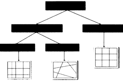
GRIDCLUS, DENCLUE, and WaveCluster [6,7, 8]. Grid-based clustering algorithms are broadly categorized into uniform grid-based clustering and non-uniform grid-based clustering. These algorithms are discussed in the following sections. Figure 2.3 depicts grids used in clustering.
Figure 2.3: Types of Data Grids
2.5.4.1 Uniform Grid-Based Clustering
Uniform grid structures partition the data space using hyperplanes that are parallel to the axis. These grid structures are also called axis-parallel grid structure. It imposes the same size grid cells and do not take into account the underlying data distribution. Then, relevant statistical information is collected for each grid cell and clustering is performed. Well-known representative examples are WaveCluster, DENCLUE, and GRIDCLUS [8,7, 6J.
2.5.4.2 Non-Uniform Grid-Based Clustering
Non-Uniform grid-based clustering algorithms impose a data adaptive grid structure. Non-Uniform grid-based clustering algorithms offer significant performance improvement over other uniform grid-based clustering algorithms. Well-known
representative examples are MAFIA, DESCRY, and MMNG [22, 11, 12J. 2.5.5 Data Shrinking Based Clustering
A gravitational transform based clustering algorithm is presented in [20). In this method, gravitational transform is applied to multi component image classification to
23
highlight the modes, or centers of high density regions, of data. The authors propose a simple model of attraction in which only mutual attraction of neighboring data points is enabled. This process is applied for a specified number of iterations. Finally, various clustering algorithms are applied to test the effectiveness of the proposed gravitational transform. Similarly, a new gravitational clustering algorithm that considers data points as an object in a gravitational field has been introduced [22]. In this algorithm, each data object is moved by simulating data movement for a specified number of iterations.
Finally, a cluster detection procedure is used to extract valid clusters at multiple levels of resolution. Following these methods, another gravitational clustering algorithm is presented in [23]. In this method, a force of attraction is applied between points, allowing each point to move slowly under the influence of the resultant force [23]. Data points that are close to each other during this movement process are merged to form a cluster. This merging process results in a hierarchical tree structure. Finally, clusters are obtained using an evaluation criterion. Further, a nonparametric clustering algorithm called CLUES is presented in [24]. It performs three functions: data shrinking, data clustering, and optimal cluster selection. The data shrinking process used in this
algorithm is derived from the gravitational clustering. The movement of each data point is determined by the median of its k-nearest-neighbors because the median is more robust than the mean. The coordinates of each data point are updated in all iterations of the algorithm. This process is repeated until convergence is observed. Finally, data partitioning and optimal cluster selection is applied.
A multi-scale uniform grid-based data shrinking and clustering algorithm that simulates data movement toward the density gradient is presented in [13, 14]. This
technique is a three part method. First, data is mapped into grid cells. Then, data points in each dense cell move toward the data centroid of the surrounding cells. This process is repeated until a specified movement threshold is achieved for a specified number of iterations. Ultimately, clusters are detected at multiple scales, and cluster evaluation is performed to obtain the final clusters.
2.6 Conclusion
This chapter explores all related research paradigm in machine learning that are part of this dissertation. It starts by discussing the localized learning paradigm and then swiftly switches the discussion to the grid-based localized learning paradigm. It then explains and discusses the data shrinking, data shrinking techniques and related issues. Next, the clustering in general and research related to the dissertation such as grid-based clustering, hierarchical clustering, and data shrinking based clustering are discussed. Furthermore, it discusses related research in supervised machine learning paradigm.
CHAPTER 3
PRELIMINARIES OF GRID-BASED LOCALIZED LEARNING
Grid-based localized learning is a specialized form of learning in which data space is divided into small partitions called grid cells by imposing a grid structure. Thus, it is necessary to formally introduce frequently used terminology in this area. In this chapter, notations, formal definitions, and other important information relating to grid-based localized learning are provided.
The remainder of the chapter is organized as follows. In Section 3.1, basic notations used in explaining the algorithmic pseudo-code is discussed. In Section 3.2, formal definitions and theorems pertaining to grid-based localized learning are explained and discussed.
3.1 Notations
Let a set X = {X;}^ be a dataset of N d-dimensional data points, where X <= 5Hd
(9? represents the set of real numbers), Xt represents an element of X. Let the element X,
(Xj £ X) be a d-dimensional vector, which is represented by the vector Xt- =
(Xj i, , Xi d) . Let the set of d-dimensions be denoted by ID) = {Dj}^ ^ For V j, 1 < j < d, let Dj be normalized between [0,1], where [0,1] c 31. Let 3) = "Dx x D2 x
x Dd be the d-dimensional data space in a unit hypercube [0,l]d c 5Rd.
Then, let n y = [0,1] denote the value domain of the dimension D; , where 1 < j < d . Let
for V T>j, Pr = [I, h) denote a right-opened interval or partition and Pc = [/, h] denote a closed interval or partition, where I denotes the lower bound and h denotes the upper bound of the partition. Let the value domain Tzy of dimension Dj be divided into K* m u t u a l l y e x c l u s i v e p a r t i t i o n s . L e t / y n = [ l j n i h j n) b e t h e nt h p a r t i t i o n , w h e r e 1 < j < d , 1 < n < . Let Ij = {/;1, — JjXi] = rhe total-ordered
set (Ij, <) that denotes the partitions in dimension Dj such that (lj x < lj>2 < ••• < lj ^j j
^hj x < hj 2 < < hj jfi j. Let Object; be the total number of data points in the grid
cell Cj. Let Volumej be the volume of the grid cell Cj. Let pj be the density of the grid cell Cj . Let Lj be the length of the ith partition of the grid cell Cj.
3.2 Formal Definitions
Using the above notations, the formal definitions of relevant terminologies in grid-based localized learning are presented here.
Definition 3.1 (Grid): A grid G on a d-dimensional unit hypercube data space D that
partitions the data space into nj=i number of partitions is given by a d-ary Cartesian product over d totally-ordered sets I\,L2> , ID- A d-dimensional grid G is given by
Equation 3.1 or 3.2:
G = LX x L2 x x ID, Eq. 3.1
G ~ «i» ^2,n2' > IJ.rij' • • • > | IJ.rij ^ /;}• Eq. 3.2
Definition 3.2 (Uniform Grid): A uniform/fixed size grid GUNIF0RM on a d-dimensional
27
Cartesian product over d totally-ordered sets I1,12, , Id such that /a = /2 = =
Id = /, K' — K for V T)j and |hjn. — (/,n;| = 1/3^, for V rij. A d-dimensional uniform
grid GUNIFORM is given by Equation 3.3 or 3.4. Figure 3.1 depicts a two-dimensional
uniform grid:
Guniform = h x h x x Id, Eq. 3.3
Guniform — {('l.nj'h,n2> — >h.nj>•••> Wi) | b.nj G 'yj- Eq. 3.4
9
CS
0.0 0.25 0.50 0.75 I
Figure 3.1: A Two-Dimensional Uniform Grid
Definition 3.3 (Non-Uniform Grid): A non-uniform grid GADAPTIVE on a d-dimensional
data space that partitions the data space D into Y\JjZi number of partitions is a d-ary
Cartesian product over d totally ordered sets llt l2, ld such that I± =£ /2 =£ =£ Id
and 11 =£ 12 =£ =£ Id- A d-dimensional data adaptive grid GADAPTIVE is given by
Equation 3.5 or 3.6. Figure 3.2 depicts a two-dimensional non-uniform grid:
Gadaptive = h x ^2 x x Eq. 3.5
T) o 6 *r> <N 0.0 0.30 0.75 1
Figure 3.2: A Two-Dimensional Non-Uniform Grid
Definition 3.4 (Grid Cell): A grid cell C in a d-dimensional grid G is a d-tuple such that
each element /y ^of the d-tuple represents a partition lj:Tlj, hj in a dimension. A
d-dimensional grid cell C is given by Equation 3.7 or 3.8 and is depicted in Figure 3.3:
C = h,n2> »b.rij' "• > Eq. 3.7
C ~ ^1 .Tii)' — » \b.ri]> ty.Tij) > — •> [h,nd> hj.ntSj- Eq. 3.8
©
in (S
0.0 0.30 0.75 1
29
Definition 3.5 (Uniform Grid Cell): A grid cell CUNIFORM in a d-dimensional uniform
grid G is a d-tuple such that each element ljn., of the d-tuple represents a partition
| lj,n}> hj,nj) a dimension where hj n. — ljn. | = 1/K, for V rij. A uniform grid cell
C u n i f o r m's given by Equation 3.9 or 3.10:
CUniform ~ {jl.nj^i ^2,n2» fy,nj> Eq. 3.9
GUniform ~ ^l,ni)> ••• > > — < [{/,n<j> fy,Tid)^" Eq. 3.10
Definition 3.6 (Non-Uniform Grid Cell): A grid cell CNON_UNIFORM in a d-dimensional
non-uniform grid G is a d-tuple such that each element IJ>N , of the d-tuple represents a
partition |ljn.,hj.n-) in a dimension where |/i;n. - ljn.| =£ 1/JC, for V n;. A
d-dimensional grid cell CN0N„UNIF0RM is given by Equation 3.11 or 3.12:
CNon-uniform = (jl.n-L' ^2,n2> Ij,nj> ••• > Eq. 3.11
CNon-uniform = h-l,nx)> — > [(/,ny fy."/) \h,nd' fy.nd)^" ^
Definition 3.7 (Empty Grid Cell): A grid cell C in a d-dimensional grid G is called an
empty grid cell if, and only if, no data point Xt = ( Xi : 1, . . . , X i j , X id) exists such
that l jn. < X i j < h jn. for V Xi;-. A d-dimensional empty grid cell C is given by Equation 3.13:
C = = Eq. 3.13
Definition 3.8 (Non-Empty Grid Cell): A grid cell C in a d-dimensional grid G is called
exists such that l jn j < Xtj < h jn. for V Xt j . A d-dimensional non-empty grid cell C is given by Equation 3.14:
C = ••• > [(/,nd» fy>,nd)^ ^ Eq. 3.14
Definition 3.9 (Neighboring/Connected Grid Cell): Let Cp and Cq be two grid cells in a
d-dimensional grid G. Let Cp and Cq represent d-tuple Cp = ..., lji P j,. •, Aj,P d) a n^
Cq =: (ji.qi' •••»b.Qj' -' Id.qd)' respectively. Grid cells Cp and Cq are called
neighboring/connected grid cells if, and only if, \lj,P j ~ Ij,q j\ ^1 for V (1 < j < d). Definition 3.10 (Non-Empty Neighboring Grid Cell): Let two d-dimensional grid cells,
Cp and Cq, be given by Cp = , IjiP), , /d>Pd) and
Cq = ,/d,qd)' respectively. Grid cells Cp and Cq are called non empty neighboring grid cells if, and only if, Cp =£ 0, Cq =£ 0 and
(1 < 7 < d).
Definition 3.11 (Grid Cell Volume): Let grid cell Ct be a d-tuple in a d-dimensional
grid G such that each element I jn. of the d-tuple represents a partition in a
dimension. Let L; be the length of the it h partition in the d-tuple. The volume Volumei of a grid cell Q is given by Equation 3.15:
Volumei = -. Eq. 3.15
1 (tiX Ld) M
Definition 3.12 (Grid Cell Density): Let Ct be a grid cell in a d-dimensional grid G , let Objecti be the total number of data points in the grid cell Q, let Volumei be the total volume of the grid cell Q and let p,- be the density of the grid cell C( . The density p; of a
31
grid cell Q is given by the ratio of Object and Volumei. ^ is expressed by Equation 3.16:
p =£^£££l, Eq. 3.16
V o l u m e i
Definition 3.13 (Dense Grid Cell): Let Cj be a grid cell in a d-dimensional grid G, let
be its density, and let Thp be a density threshold. Grid cell C; is called a dense grid cell if, and only if, the density p£ is greater than or equal to Thp. It is expressed by
Equation 3.17:
Sparse, if pi <Thp
Dense, if pi>Thp Eq. 3.17
Ci =
Definition 3.14 (rt h Rank Neighbor): Let grid cell C and Cp be represented by d-tuples
Id.ua) and respectively. Grid cell Cp is called the r rank neighbor of the grid cell C if, and only if the following condition is satisfied. This condition is expressed in Equation 3.18:
fh.nj + 1 or /,-n. - 1, V j, (1 < ;' < r)
t h
l w V;', (r + 1 < ;' < d)' Eq.3.18 Definition 3.15 (Data Centroid): Let Cj be a grid cell that contains a set Xj of k data
points Xj = {Xji, Xi k], where Xj c X. The data centroid q of the grid cell Cj is given by Equation 3.19:
Eq. 3.19 Definition 3.16 (Overlapping-Cell): Let Q be a grid cell that contains a set Xj of k data
points Xj = (Xjlr... where Xj c X. The grid cell Cj is called an
Definition 3.17 (Non-Overlapping Cell): Let be a grid cell that contains a set X* of k
data points Xj = {Xil( where Xj c X. The grid cell Q is called a
non-overlapping cell if it only contains the training samples of a single class.
Definition 3.18 (Micro-Partition): Let mr be a micro-partition that contains k data
points (mr l,mr u, ,mrk). A micro-partition mr is a smallest non-overlapping
unit of data points in which data points are in close proximity (| mr u — mr(U+1)| « f,
where £ is a small number) with each other.
Definition 3.19 (Average Linkage): Let mr, and mr+1 be two contiguous
micro-partitions that are given by sets mr = (mr l,,.., mr k) and nv+j = (mr+11,..., nVn.fc).
respectively. The average linkage between two contiguous micro-partitions is defined by Equation 3.20:
AVERAGE{mr,mr + 1) = - mr+1J|. Eq. 3.20
Definition 3.20 (Centroid Linkage): Let mr, and mr + 1 be two contiguous
micro-partitions in the transformed space that are given by sets mr = (mr l,..., mr k) and mr+1 = (mr+11,....,mr+l k,), respectively. The centroid linkage between two contiguous micro-partitions is given by Equation 3.21:
CENTROID(mr,mr + 1) = |m^— mr + 1\, Eq. 3.21
where mr,i, and m
(r+i)j-Definition 3.21 (Ward Linkage): Let mr, and mr+1 be two contiguous micro-partitions
in the transformed space that are given by sets = (mr l,..., mr k) and mr+1 =
mr+i,k )> respectively. The ward linkage between two contiguous
33
WARDimr.mr^) = (k * Eq. 3.22
where rn~ = ±£f=1 and m~^ = ^2f= 1 m
(r+i)j-Definition 3.22 (Z-Score Normalization): Assume j4 is a numeric attribute, its mean
is nA, its variance is aa, and a specific attribute value is ValueA. Attribute value ValueA is mapped to a new attribute value Value'A by computing the following equation:
ValueA = Eq. 3.23
OA
Definition 3.23 (Min-Max Normalization): Min-max normalization performs a linear transformation on the attribute values. Assume A is a numeric attribute, its maximum value is MaxA, its minimum value is MinA, and a specific attribute value is ValueA. Attribute value ValueA is mapped to a new attribute value ValueA in the range of [NewMinA , NewMaxA] by computing the following equation:
Valued = N e w M i ^
A (MaxA- M i nA) A M
Theorem 1: Grid-Based Neighborhood
Let G be a grid on a d-dimensional data space D that partitions the data space into mutually exclusive intervals or partitions. Let Cu be a d-dimensional grid cell that is a d-tuple Cu = h,n2> - //inj, •••»^d,nd) such that each element of the tuple
represents a partition in the corresponding dimension. Then, a d-dimensional grid cell Cu can have distinct neighboring grid cells that are given by Equation 3.25, where Sj is the number of changes in the partition index value lj>Tlj in dimension 2that satisfies the neighborhood criteria:
Proof: Let a d-tuple (jxi P l, —, lj,P j, • •, ^d,pd) represent a grid cell Cp. The grid cell Cp is
the neighboring grid cell of cell Cu = (/lni, lj n j,..., /dj„d) if, and only if, lj p. =
| I j n . — 1 or I j n. + 1 or I j n. , V j, (1 < j < d). Therefore, each element I j> p. of a
neighboring grid cell Cp can have a maximum of three values that satisfy the
neighborhood criterion. If Sj represents all possible changes for dimension 2); , then the
number of neighboring grid cells is given by Equation 3.26:
cNeighbor = (^1 * - * Sj * ... * Sd) - 1, Eq. 3.26
(•Neighbor = (^1 * - * Sj * ... * Sd) - 1 = Y\j=i Sj - 1. Eq. 3.27
It should be noted that -1 in Equation 3.26 indicates I jp. = I jn. V j, (1 < j < d)
CHAPTER 4
GRID-BASED LOCALIZED LEARNING FOR DATA PREPROCESSING
Most real world data is low quality, and the data used for the data mining tasks may be incomplete, noisy, inconsistent, and sparse. Consequently, it is necessary to improve the quality of the data by addressing these data deficiencies prior to data analysis through a series of steps collectively called data preprocessing. There are several
challenges in preparing this data for data mining tasks such as clustering and
classification among others. These challenges are categorized into challenges related to the characteristics of the raw data such as noisy, missing, and inconsistent data values and into challenges related to the characteristics of the data such as sparseness and the curse of dimensionality in multidimensional data space.
Both these sets of challenges severely affect the data analysis and may lead to low quality and misleading conclusions. Therefore, data preprocessing is necessary before performing any type of data mining tasks. Many techniques have been developed to handle the noise, incomplete and inconsistent data. Similarly, many techniques have been developed to mitigate the effect of the curse of dimensionality and the sparseness of the data. The sparseness of the data, which is caused by the curse of the dimensionality, severely undermines the performance of data mining algorithms. Because of this potential deterioration of the performance, one emphasis of the research presented in this
dissertation is to develop better sparseness reduction algorithms and frameworks and integrate them with the clustering algorithms.
The remainder of this chapter is organized as follows. In Section 4.1, a brief explanation of various data preprocessing techniques is provided. In Section 4.2, a discussion about data sparseness, its detrimental effects and sparseness reduction techniques are provided. In Section 4.3, research motivation for the non-uniform grid-based sparseness reduction technique is discussed. In Section 4.4, an experimental study is presented to demonstrate the advantages of the non-uniform grid-based sparseness reduction technique. In Section 4.5, the conclusions of this chapter are presented.
4.1 Data Preprocessing
Data preprocessing refers to the process of improving the quality of data for the ease of the data mining or knowledge discovery process. Data preprocessing is a
collection of a wide variety of operations. The process includes data cleaning operations, which usually compose the first set of operations performed on the data. The second set of operations is called data transformation operations, which converts the data into a specified format. The third set of operations is referred to as data reduction operations, which includes operations to reduce data such as aggregation and dimensionality
reduction. The fourth set of operations is referred as data shrinking operations. It includes operations regarding sparseness reduction. Data processing can improve the overall quality of data and the data mining tasks for knowledge discovery [2]. A brief discussion about all four sets of operations is given below.
1. Data Cleaning: Data cleaning refers to the set of operations performed to clean the data by removing noise from the data, filling in missing data values, and resolving
37
inconsistent data values. Common noise removal operations are binning, regression, and clustering. Common operations for filling in missing values involve the use of a global constant, the use of an attribute mean, and the use of a most probable value. Common operations for resolving inconsistent values are the use of domain knowledge and the use of rules discovery to find inconsistent relationships [2]. 2. Data Transformation: Data transformation refers to the set of operations that
transform the data into representations which are appropriate for the data mining task at hand [2]. The set of data transformation operations consists of data smoothing, aggregation, generalization, normalization, and attribute construction. Data
smoothing involves binning, regression, and clustering. Data aggregation involves data summarization. Data generalization involves replacing raw data by higher level concepts. Data normalization involves scaling data values into the specified range. Attribute construction involves extracting new attributes from the given set of attributes.
3. Data Reduction: Data reduction refers to the set of operations that are applied to obtain a reduced representation of the data without seriously compromising the integrity of the original data [2], Data reduction operations consist of data aggregation, attribute subset selection, dimensionality reduction, and sample
reduction. Data aggregation involves data summarization. Attribute subset selection involves removing irrelevant, weak, or redundant attributes. Dimensionality reduction involves reducing dimensions by applying wavelet transform, principal component analysis, and Fourier transform, among other methods. Sample reduction involves the use of histograms, clustering, parametric models, and sampling techniques [2].