UCLA
UCLA Electronic Theses and Dissertations
TitleApplication of Machine Learning Algorithms in Predicting Credit Card Default Payment
Permalink https://escholarship.org/uc/item/9zg7157q Author Gui, Liyu Publication Date 2019 Peer reviewed|Thesis/dissertation
UNIVERSITY OF CALIFORNIA Los Angeles
Application of Machine Learning Algorithms in Predicting Credit Card Default Payment
A thesis submitted in partial satisfaction of the requirements for the degree
Master of Applied Statistics
by
Liyu Gui
c
Copyright by Liyu Gui
ABSTRACT OF THE THESIS
Application of Machine Learning Algorithms in Predicting Credit Card Default Payment by
Liyu Gui
Master of Applied Statistics
University of California, Los Angeles, 2019 Professor Yingnian Wu, Chair
This paper aims to apply multiple machine learning algorithms to analyze the default pay-ment of credit cards. By using the financial institutions client data provided by UCI Machine Learning Repository, we will evaluate and compare the performance of the model candidates in order to choose the most robust model. Moreover, we will also decide which are important features in our best predictive model.
The thesis of Liyu Gui is approved.
Frederic R Paik Schoenberg Vivian Lew
Yingnian Wu, Committee Chair
University of California, Los Angeles 2019
TABLE OF CONTENTS
1 Introduction . . . 1
2 Data Exploratory Analysis . . . 3
2.1 Data Set Information . . . 3
2.2 Attribute Information . . . 3
2.3 Exploratory Analysis . . . 5
3 Methodology . . . 9
3.1 Data Preprocessing Technique . . . 9
3.2 Logistic Regression . . . 10 3.3 Decision Tree . . . 12 3.4 Random Forest . . . 14 3.5 AdaBoosting . . . 15 3.6 Gradient Boosting . . . 17 3.7 Neural Networks . . . 18 4 Model Analysis . . . 20 4.1 Logistic Regression . . . 21 4.2 Random Forest . . . 21 4.3 AdaBoosting . . . 24 4.4 Gradient Boosting . . . 27 4.5 Neural Network . . . 29 5 Conclusion . . . 32
LIST OF FIGURES
2.1 Credit Card Customer - target value . . . 6
2.2 Non-Defaulter vs Defaulter within Specific Credit Limit Group . . . 7
2.3 Sex vs Defaults Payments . . . 7
2.4 Education vs Defaults Payments . . . 8
3.1 Graph of Logistic Regression . . . 11
3.2 Decision Tree Algorithm . . . 12
3.3 Random Forest Algorithm . . . 14
4.1 Python Code of Splitting Data Set . . . 20
4.2 ROC Curve of Random Forest Model . . . 22
4.3 Confusion Matrix of Random Forest Model . . . 23
4.4 Performance Index of Random Forest Model . . . 23
4.5 Important Features in Random Forest Model . . . 24
4.6 ROC Curve of AdaBoost Model . . . 25
4.7 Confusion Matrix of AdaBoost Model . . . 25
4.8 Performance Index of AdaBoost Model . . . 26
4.9 Important Features in AdaBoost Model . . . 26
4.10 ROC Curve of Gradient Boosting Model . . . 27
4.11 Confusion Matrix of Gradient Boosting Model . . . 28
4.12 Performance Index of Gradient Boosting Model . . . 28
4.13 Important Features in Gradient Boosting Model . . . 29
4.14 Neural Network Architectural Diagram . . . 30
LIST OF TABLES
2.1 Missing Data . . . 5 2.2 description of first 5 columns . . . 5
CHAPTER 1
Introduction
According to the Federal Reserve Economic Data, the delinquency rate on credit card loan across all commercial banks is at all-time high for the past 66 months, and it is likely to continue to climb throughout 2019 [1]. The delinquency rate indicates the percentage of past-due loans within the borrowers’ entire loan portfolio. The climbing delinquencies will result in significant amount of money loss from the lending institutions, such as those commercial banks. Therefore, it is very crucial for banks to have a risk prediction model and be able to classify the most relative characteristics that are indicative of people who have higher probability to default on credit card loans. A robust model is not only a useful tool for the lending institutions to make decision on credit card applications, but it can also help the clients to aware of the behaviors that may damage their credit scores.
Nowadays, machine learning algorithms are the most popular technique to build models. The name machine learning was coined in 1959 by Arthur Samuel, who defined it as “the field of study that gives computers the ability to learn without being explicitly programmed” [2]. In 1998, Tom Mitchell, another well-known machine learning scholar, gave us a narrower definition regarding machine learning, compared to Samuel’s. He stated the process of learning problem is that “a computer program learns from experience E with respect to some task T and some performance measure P, if its performance on T, as measured by P, improves with experience E” [2]. Frankly speaking, the primary aim of machine learning is to train the computers so that they are able to observe the previous data or examples that we provide, and automatically learn from them by identifying the patterns in order to make decisions in the future. When choosing the most suitable model, there are many factors that contribute to the decision making. No one can say that one algorithm is always better
than the other one. In a nutshell, no one algorithm always work best for every problem or one type of problems, and we should try many different algorithms for our problem; then carefully evaluate and compare their results to select the best algorithm.
Machine Learning algorithms can be divided into two broad categories: supervised learn-ing and unsupervised learnlearn-ing. Startlearn-ing from the analysis of the trainlearn-ing data set, the supervised machine learning algorithms make predictions on the output values in the test data set. These types of algorithms are usually used to build the predictive models. On the other hand, the unsupervised machine learning algorithms are applied when the given training data set is neither labeled nor classified. Unlike the supervised learning, the unsu-pervised learning deals with the data that has unknown possible outputs and looks for the hidden structures from the unlabeled data instead of figuring out the correct answers [3].
The objective of this research paper is to find the best model that is able to identify whether a credit card holder will default next months payment based on the demographic attributes of the card holder and his/her history of past payment. Since we have known input and output values and expect a predictive model at the end, the supervised learning should be chosen when implement machine learning algorithms. As a result, the lending institutions will be able to use our final model to reduce the high delinquency rate by correctly classifying the credit card defaulters and non-defaulters. In order to achieve my goals, the following steps will be followed:
1. Download dataset from UCI Machine Learning Repository website 2. Clean the original data and perform exploratory data analysis
3. Train 5 different supervised learning models and neural network model 4. Compare and evaluate the predictive accuracy among all models 5. Make conclusion based on the results
CHAPTER 2
Data Exploratory Analysis
2.1
Data Set Information
The data set for training and testing is obtained from UCI Machine Learning Repository webpage. It was donated to UCI Repository in 2016 by Taiwans institutions, Chung Hua University and Tamkang University. This data set contains the information of customers default payment in Taiwan. There are 30,000 different instances and 25 attributes total; each instance represents one customer, and attributes consist demographic information about the customers and their past payment history from April to September.
2.2
Attribute Information
ID: unique identification number assigned to each customer LIMIT BAL: amount of given credit access line
SEX: gender (1 = male; 2 = female)
EDUCATION: highest degree obtained (1 = graduate school; 2 = university; 3 = high school; 4 = others; 5 = unknown; 6 = unknown)
MARRIAGE: marital status (1 = married; 2 = single; 3 = others) AGE: age in year
PAY 0: monthly payment record in September PAY 2: monthly payment record in August PAY 3: monthly payment record in July
PAY 4: monthly payment record in June PAY 5: monthly payment record in May PAY 6: monthly payment record in April BILL AMT1: total amount owed in September BILL AMT2: total amount owed in August BILL AMT3: total amount owed in July BILL AMT4: total amount owed in June BILL AMT5: total amount owed in May BILL AMT6: total amount owed in April
PAY AMT1: amount of previous payment in September PAY AMT2: amount of previous payment in August PAY AMT3: amount of previous payment in July PAY AMT4: amount of previous payment in June PAY AMT5: amount of previous payment in May PAY AMT6: amount of previous payment in April
default payment next month: whether a customer is defaulted on next months payment or not (1 = defaulter; 0 = non-defaulter)
The columns from PAY 0 to PAY 6 represent the repayment status in each month from April to September: -1 indicates paying duly for one month; -2 indicates paying duly for two months; . . . ; -x indicates paying duly for x months. The positive number shows that how many months the payment has been delayed. For example, 1 means that the payment has been delayed for 1 month; 2 mean that the payment has been delayed for 2 months; . . . ; x means that the payment has been delayed for x months.
In order to unify the variable name, I will use PAY 1 as a substitute for PAY 0 to represent the repayment status in September. The last column “default payment next month” will be used as the output of the final predictive model.
2.3
Exploratory Analysis
The column “ID” consists randomly generated ID values by the lending institutions and it does not affect the customers ability to pay back the bill. Hence, I remove this column from the data set. Besides this column, no other column contains redundant information, poorly formatted, or has no impact on customers ability to pay for the balance. Therefore, I have 23 attributes left to build the model and the last column in the data set will be my target column.
First of all, I checked whether this data set includes any missing data.
Table 2.1: Missing Data
default.payment.next.month PAY 6 LIMIT BAL ... PAY AMT3 PAY AMT4 PAY AMT5
Total 0 0 0 ... 0 0 0
Percent 0 0 0 ... 0 0 0
Table 1 indicates that there is no missing data in the entire data set. After the cleaning process, we can look into more details about the data.
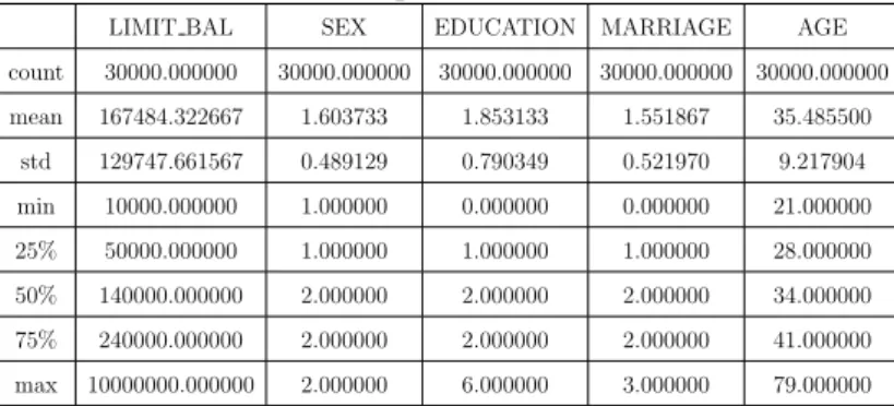
Table 2.2: description of first 5 columns LIMIT BAL SEX EDUCATION MARRIAGE AGE count 30000.000000 30000.000000 30000.000000 30000.000000 30000.000000 mean 167484.322667 1.603733 1.853133 1.551867 35.485500 std 129747.661567 0.489129 0.790349 0.521970 9.217904 min 10000.000000 1.000000 0.000000 0.000000 21.000000 25% 50000.000000 1.000000 1.000000 1.000000 28.000000 50% 140000.000000 2.000000 2.000000 2.000000 34.000000 75% 240000.000000 2.000000 2.000000 2.000000 41.000000 max 10000000.000000 2.000000 6.000000 3.000000 79.000000
From Table 2 we can see that the average amount of given credit access line is 167,484 with an extremely high standard derivation close to 130,000, which can be explained by the large number of maximum credit card limit of 1 million. The average education level is 1.853, which indicates that most customers obtained bachelor or master degrees. More customers are either married or singled, compared to the number of unknown. The median age is 35.5
with 9.2 standard deviation. The youngest customer is 21 years old, while the oldest is 79 years old.
Figure 2.1: Credit Card Customer - target value
6,636 customers (approximate 22.12% of the entire data set) will default in the next months payment, while 23,364 will not default. This result is quite reasonable because the difference is insignificant so that this data set should not have much bias information and can be used in our further analysis.
The amount of credit line may be a good indicator of defaulting behavior. Intuitively, people who have good credit score are likely given high credit line compared to those who have very low credit score. On the other hand, people who have default payment in the past are usually hard to raise their credit lines. Therefore, the number of defaulters with credit lines in the top 25% should be much smaller than the number of defaulters having low credit line.
Figure 2.2: Non-Defaulter vs Defaulter within Specific Credit Limit Group
Figure 2 expresses the number of defaulters and non-defaulters in each different credit limit group. The plot confirms our conjecture about the relations between number of default-ers and credit limit. When the credit limit is below the average, the number of defaultdefault-ers is obviously higher than the number of non-defaulters. The difference nearly doubles for some specific low credit limit. As the credit limit goes beyond the average, the number of non-defaulters gradually increases within each group and most of them are larger than the number of defaulters. The amounts of 50,000 credit limit has the largest defaults number, as well as 20,000 and 30,000 credit limits.
Next, I will check the impact of sex on the number of default payments.
The bar chart suggests that the number of female customers are more than the male cus-tomers, and the number of female defaulters are slighter higher than males. Although it is hard to find a tenable reason that sex could have any impact on the default payment, this column will still be included in the data set for training the models.
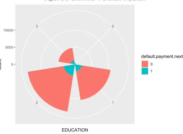
Figure 2.4: Education vs Defaults Payments
On the other hand, no evidence of significant education level’s impact was found in the polar area chart of the education level against defaults payment, though we normally believe that people who obtained high degrees tend to pay their loans duly because they may earn much more than those who never earned a degree. Once making money is not concerned anymore, the loans should not be worried as well.
CHAPTER 3
Methodology
3.1
Data Preprocessing Technique
One major drawback in this data set is that the numerical features are all measured in different units. Therefore, data standardization, an effective data preparation scheme for tabular data, should be considered so that the comparison between measurements can be more accessible when building models, especially the neural network models. Being a general technique in machine learning, standardization is a process of re-scaling the feature values in order to make the new inputs follow the standard normal distribution with
µ= 0 and σ= 1 (3.1)
where µ is the mean and σ is the standard deviation. The standard normal curve is sym-metrical, centered about its mean 0 with its spread determined by the standard deviation 1 [4]. The formula for calculating the standard score z is given below:
z = x−µ
σ (3.2)
This rescaling technique is often used in the gradient descent algorithm, which is an opti-mization algorithm used in logistic regression, SVMs, neural networks etc. Before rescaling, different features tend to have different units; when training the model, those with higher values will inevitably learn faster than others because large value xj will affect the weight updates rate as follow:
∆wj =−η ∂J ∂wj =η X i (t(i) −o(i))x(ji) (3.3) where t is the target value (class label), η is the learning rate, and o is the actual output value.
Besides the gradient descent algorithm, many other algorithms will be optimized by the data standardization, such as those I mentioned above and k-nearest neighbors. The implementation of KNN algorithm is to calculate the average of total distance between the numerical target value and its k nearest neighbors. When calculating the distance by using Euclidean function, the feature with larger values will have a much higher influence on the distance calculated. In this case, one feasible solution to optimize the data is to standardize the training set [4].
3.2
Logistic Regression
The supervised machine learning can be further divided into two sub-groups: classification and regression. The problem with categorical outputs are grouped into classification problem, while the outputs of a regression problem are numerical. In this research, the output is either credit card defaulter or non-defaulter. The problem, hence, should be grouped into classification problem. Whereas the logistics regression model has the word “regression” in its name, it is actually one of the most simple and popular classification algorithms [5].
The logistic regression algorithm is based on the concept of probability of the predicted output which lies within 0 and 1 range:
0≤hθ(x)≤1 (3.4)
The cost function that a logistic regression uses is called the “sigmoid function,” which has the formula as follow:
σ(z) = 1
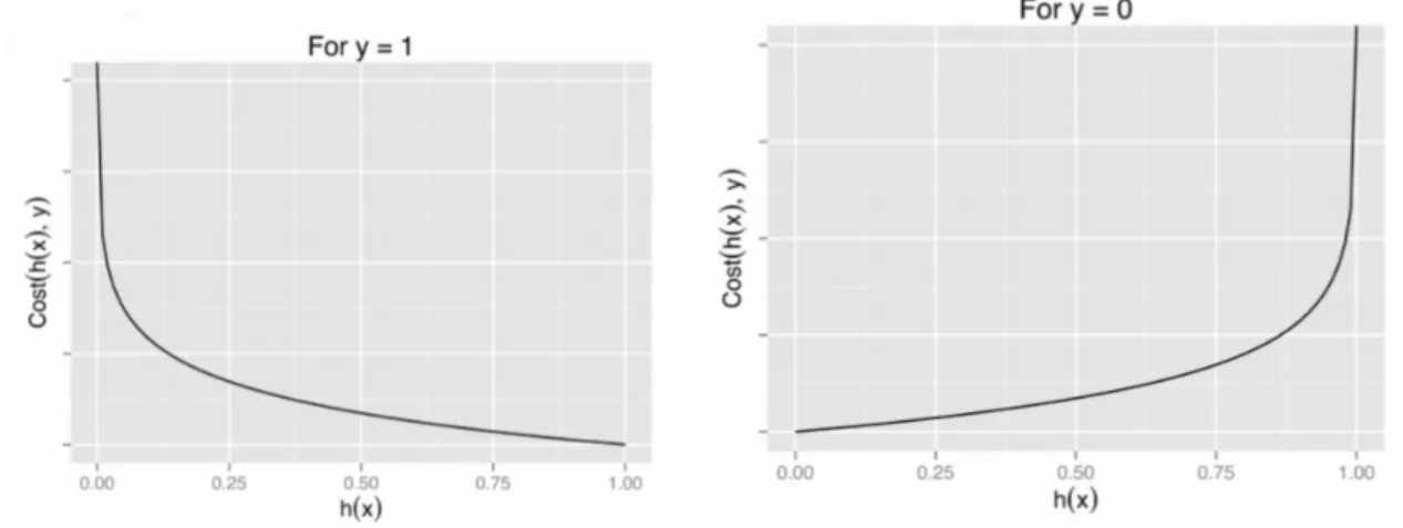
This function maps the probability of the predicted value between 0 and 1. As the predicted probability will return a value between 0 and 1, we must pick the most suitable cut-off point, as named as the threshold value, for segregating if the customer will default the payment or not. If the probability is below the selected threshold value, the corresponding output will be classified as 0, the non-defaulter group or vice versa. The cost function for logistic regression can be visualized as well.
Figure 3.1: Graph of Logistic Regression
The stepped cost functions can also be compressed into one single function:
J(θ) =− 1
m X
[y(i)log(hθ(x(i))) + (1−y(i))log(1−hθ(x(i)))] (3.6) I shall be discussing the method of how to minimize the cost function J(θ) in depth in a later section.
3.3
Decision Tree
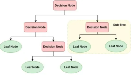
Figure 3.2: Decision Tree Algorithm
The discipline “Decision Tree” is aptly named; it is a tree-like structure that allows the system to make decision by weighing the possible actions. The trees can be either binary or non-binary. Starting with a single node (called “root”) at the top, a decision tree branches into all possible outcomes. Each feature from the data set is an internal node, which leads to the additional nodes until the leaf is reached by testing the characteristics of each instance [5]. The corresponding branch is chosen based on the testing result. At the end of branches, the node does not split anymore and a decision is finally made for that instance.
There are two types of decision tree: classification tree and regression tree. As the name goes, the classification tree classifies the target into a category, while the regression tree predicts continuous values.
In order to decided which features should be used in the tree model, the system usually use a cost function to test and try different splits and choose the split that having lowest cost. The cost function here will calculate the accuracy that each candidate split has; the lower cost is, the better split is. The method of chosen the specific split is also defined as greedy algorithm that minimizes the cost function and makes the optimal choice at each
local stage [6]. The simple squared error function is commonly used for a regression tree:
E =X(Y − Yˆ)2 (3.7)
whereY is the actual value and ˆY is the predicted value. For a classification tree, I will use
Gini Index Function as my cost function:
E =X[pk × ( 1 − pk) ] (3.8)
where pk is the proportion of observations with target variable value k. In the binary tree,
k takes value of 0 and 1 [7]. In this paper, the leaf is whether the credit card holder is a defaulter or non-defaulter so I will focus on the classification trees.
A tree can grow forever if we do not tell the system when to stop. In general, overfitting will occur when a tree is too complex with large number of splits. There are a few ways to solve this problem. One method is to set a minimum number of training data sets on each leaf. If the inputs are less than a certain number on one leaf, we will get rid of this leaf; if the inputs equals to this number, we can make a decision. The other way is to set a maximum number of nodes on root to leaf path [7].
Moreover, we need to trim the branches by “cutting” the less important nodes when the tree grows arbitrarily. This pruning process can start at either root or leaves. If we start at root, the weakest link pruning method can be used by comparing the size of the nodes’ sub-tree in order to remove those with less weight. If we start at leaves, the reduced error pruning is another practical method, which removes each leafs most significant node until the accuracy changes.
3.4
Random Forest
Figure 3.3: Random Forest Algorithm
While the decision tree algorithm has many advantages, it also has many drawbacks. For example, the decision tree that is returned by greedy algorithm may not be the globally optimal tree. In this case, building multiple trees is in demand. The samples are randomly selected and replaced for the individual tree and the final model is built by merging all trees together so that the result should be more accurate and stable than one decision tree. The process is also named as “bagging” method [8].
Similar to the decision tree algorithm, the random forest can be also used for both classification models and regression models. I will focus on the classification model here. On the other hand, the random forest algorithm looks for the best suitable feature among a random subset of features rather than the best possible feature when splitting a node from multiples trees. Sklearn, a Python built-in function, is great tool to measure the importance of each feature by calculating the reduced impurity of all tree nodes that contain this feature and scale the results so that the sum of them is equal to 1. The intention we need to compute the importance is to avoid overfitting problem by removing the insignificant features that only have trivial contribution to the entire prediction process.
optimize. In order to increase the prediction accuracy, we can increase the number of trees before computing the average of predictions. However, there is a drawback in this process -as the number of trees the algorithm built incre-ases, the learning speed of model will decre-ase simultaneously. Beside this parameter, we can also consider minimizing the number of leafs or maximizing the number of features that a model required to split a node.
There are three parameters in Sklearn affecting the models speed: “n jobs”, “random state”, and “oob score”. The first one shows the number of processor that the system can use. If the same parameters and data set are given, the model should be able to reproduce the results when it has a specific value of “random state”. Similar to leave-one-out cross-validation method, “oob score” is a cross validation method for random forest model to measure the prediction error. Once the data set is divided into training set and test set. The values in the latter set are used to evaluate the models performance and called the out of bag samples.
3.5
AdaBoosting
AdaBoost, also referred to as Adaptive Boosting, is the most fundamental Boosting algorithm to solve classification problems. It combines a set of “weak classifiers” into one “strong classifier”. In order to accomplish this, AdaBoost gives unequal weight to instances based on their classification’s result. The instances that are difficult to classify are given more weight while those that are easy to classify are put less weight. The weak classifiers in AdaBoost are single-split decision trees. Those single splits are called decision stumps [9]. The function for linear weighted combination of weak classifiers to boost the performance can be represented as F(x) = sign( M X m=1 θmfm(x)) (3.9)
where fm(x) denotes the mth weak learner and θm is the corresponding weight.
When we simply guess the outputs of a data set are all 1s or 0s, we will have the best accuracy rate. For example, if 70% of the points are 0s in the data set, we will have 70%
accuracy if we guess 0 for every data point. Decision stumps optimize this performance by dividing the points into two subsets according to a single feature. After selecting a feature and threshold, the decision stump then continues to divide the points into two subsets on both sides of the threshold.
Lets consider a data set with n points, where
xi ∈Rd, yi ∈ {−1, 1} (3.10) -1 shows the negative class and +1 represents the positive class. Each point is initially equal weighted, so that
w(xi, yi) = 1
n, i= 1, ..., n (3.11)
First, we fit multiple weak classifiers to the data set and choose the classifier with the lowest weighted classification error, defined as
m =Ewm[1y6=f(x)] (3.12)
The next step is to compute the weight θm for this weak classifier:
θm = 1 2ln( 1−m m ) (3.13)
The weight of a classifier is positive if this classifier has an accuracy higher than 50% and vice versa. Moreover, the classifiers with higher accuracy has larger weight than those with lower accuracy. Although the weight of a classifier with lower than 50% accuracy is negative, we can obtain the accuracy that higher than 50% by flipping the sign of its prediction. By doing so, each classifier, no matter how accuracy it can make, has some contribution to the final prediction. The accuracy of random guessing is 50% so we avoid any accuracy of classifier to equal to 50%; otherwise, the classifier has no contribution to the final prediction [10].
Following the above step, we give a new weight for each point following the formula:
wm+1(xi, yi) =
wm(xi, yi)exp[−θmyifm(xi)]
Zm
(3.14) where Zm is a normalization factor that ensures a probability density function with total probability of 1. The data point that is assigned higher weight so that it will have higher probability to occur in the subsequent subset is defined as misclassified point [11]. In this case, the exponential term must be larger than 1 if the misclassified point is form a classifier containing positive weight and vice versa.
At last, we repeat these three steps for each iteration m = 1, ...,M.
3.6
Gradient Boosting
In the prior section, we already know that boosting is a gradual and sequential technique to convert weak classifiers to strong classifiers by learning from the errors of the former predictors. Each data point is given unequal weight so its probability of occurring in following models is different [12]. The higher the error, the higher the probability. There are numerous methods to choose the predictor/feature, such as classifiers, decision trees etc . As we repeat the learning steps to have new predictors, the time spent on getting close to the actual outputs decreases. Nevertheless, we should also avoid the overfitting problem that can be triggered by the predictors which are too close to the actual outputs.
Gradient Boosting, as a variant of AdaBoosting algorithm, can be applied in both classi-fication and regression problems by combining a set of weak predictors, (e.g. decision trees). Like other supervised learning algorithm, the objective of Gradient Boosting is to minimize the loss function. Let us define a loss function mean squared error (MSE):
Loss=M SE =X(yi−yip)
2 (3.15)
whereL(yi, yip) is loss function, yi is theith target value, andypi is the corresponding predic-tion. We can minimize the mean squared error by update the predictions based on a learning
rate based on the following formula:
yip =ypi +α×δX(yi−yip)
2/ δyp
i (3.16)
where α is learning rate and P
(yi −yip) is sum of residuals. Once the sum of residuals reaches close to 0, the predicted values should be close to the actual values. This is the process of gradient boosting.
Briefly speaking, gradient boosting enhances a model’s performance by observing the patterns in residuals and let the test loss reach its minimum value by minimizing the loss function. The stopping criteria is usually set at the point when residuals do not have patterns anymore.
3.7
Neural Networks
Neural Networks can be used for carrying out a variety of tasks. The two most powerful applications are clustering and classification. Usually the classification missions are known as supervised learning. In order to perform a classification, the training data sets are required to be labeled, which means each training data should be lucidly assorted to one class. On the other hand, for a clustering tasks, labeled data sets are not necessary, the neural networks here are used for identifying the similarities of input data [13]. We usually call this kind of learning unsupervised learning.
Neural Networks are composed of multiple layers of neurons. Each neuron absorbs in inputs from data and compute weighted sum of them, in this way, they are able to attach importance to each input. Subsequently, the result of this sum of product for each neuron would go through an activation function, thereby determining the input for next hidden layer or output layer. In deep neural networks, each layer takes inputs from the outputs of previous layer.
One critical task for neural networks training is tuning the value of the weights attached to each input out of consideration for minimizing the error of our networks. One of the best
way to perform such task is gradient descent. As we know, along with the slope direction, the function is changing most rapidly. By using this fact, we take derivative for each weight and tuning them towards this direction until the error reach its local minimum.
Say we have a neuron defined as:
Y =X(weight×input) +bias (3.17)
where Y can take any value ranging from −∞ to +∞. This activation function converts an input of a node to an output signal, which is used as the input in the following layer. In the case that the result of activated or not is based on the comparison between Y and a threshold, a “step function” should be used to make an activation function for a neuron. If the value of Y is greater than the threshold, the activation function is activated and equals 1; otherwise, the activation function equals 0 [14].
Sigmoid function is a type of logistics function with S-shaped graph. Currently, the numerous types of sigmoid function are widely applied in the neural networks as an activation function. Unlike step function, the combinations of sigmoid function are always nonlinear, no matter they are binary activation or not. Moreover, the range of the activation function is from 0 to 1 rather than−∞ to +∞.
The last type of activation function I would like to introduce is ReLu function. If the input is positive, the function will return a value and 0 otherwise; this can be written as:
A(x) =max(0, x) (3.18)
Like sigmoid function, ReLu is also nonlinear and the its combinations are nonlinear as well. The range of ReLu is from 0 to +∞. Sometimes when we have a large neural network with numerous neurons, a sigmoid function can nearly cause all neurons to activate in an analog way. ReLu, in this case, is able to make a few neurons not activate. Another advantage that ReLu has is that it involves more simple and straightforward mathematical operations than sigmoid function [14].
CHAPTER 4
Model Analysis
In order to obtain the test validation of our models, I divide my data set into two parts with an 70-30 split: 70% of data instances are the training data while the rest of 30% are test data. We already know that there are total 30,000 different instances in this case. Therefore, the training set contains 21,000 data points and the test set contains 9,000 data points. The Python code to split data set is shown below:
Figure 4.1: Python Code of Splitting Data Set
where the parameter random state is set as 42 which triggers the internal random number generator and decide how to split train and test data set. Since there is no missing or invalid data, we do not need to impute missing values to the mean.
Two major methods will be used in this paper for analyzing the performance of each model. The first one is confusion matrix, which is generally used as a performance measure-ment for machine learning classification problem [12]. The confusion matrix not only tells us the precision and accuracy of a model, but it also helps us to plot the Receiver Operat-ing Characteristic (ROC) curve, which is another key performance measurement for machine learning models. I will talk about these two measurements with details in the further sessions as I start analyzing the models.
4.1
Logistic Regression
The logistic regression model is the simplest model in our case. The “hinge” loss func-tion is used in this linear model to evaluate how well this algorithm models my test set. Unlike other loss functions, the hinge loss penalizes significantly heavily on the incorrect predictions and correct with less confident predictions. The model’s prediction correction rate is 0.769444, which indicates that about 76.44% of test sets are predicted correctly by the logistic regression model.
4.2
Random Forest
In the random forest algorithm, we generally want as many trees as we can to get a better model. However, the increased computational cost limits the number of trees as the error rate will not decrease significantly after a certain number of trees. Furthermore, we prefer larger trees rather than smaller trees so that the depth of tree is big enough to convey information by splitting each node. The average number of nodes in this case is 6066 with average maximum depth 40.
Before looking at the confusion matrix and ROC curve, I want to clarify some crucial terminologies. First is the term “recall”, which measures true positive rate of the model based on the formula:
Recall/Sensitivity = T rue P ositive
T rue P ositive+F alse N egative (4.1)
The second term is “specificity” which indicates the false positive rate of the model based on the formula:
Specif icity = F alse P ositive
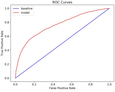
A good model should bow up to the top left of the ROC plot because the smaller values on the x-axis represents lower false positive values and larger value on the y-axis indicates higher true positive values.
Figure 4.2: ROC Curve of Random Forest Model
The ROC curve of random forest is close to the diagonal, which is the baseline here, so the test is not strongly accurate as an ideal ROC curve should as close to the top and left-hand borders as possible. We can see that any increase in true positive rate will be accompanied by a decrease in false positive rate.
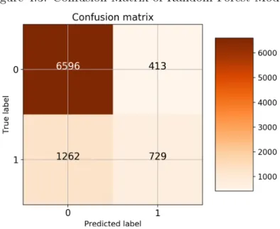
Figure 4.3: Confusion Matrix of Random Forest Model
Figure 4.4: Performance Index of Random Forest Model
According to the confusion matrix and performance index of random forest model, there are 729 true positive values and 6596 true negative values. The recall for test set is 0.366148 and precision for test set is 0.638354. The accuracy classification score for test set is 0.813889, which means that about 81.39% of data instances in the test set are predicted correctly by our random forest model, which is trained based on the training set.
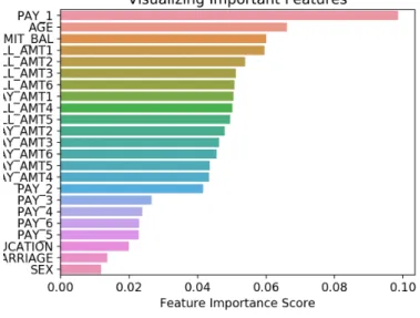
Figure 4.5: Important Features in Random Forest Model
The above graph helps us to visualize the important features that play significant roles in predicting the output. The results are quite similar to our conjecture made in the previous chapter. The feature “Pay 1” has the highest feature importance score, which indicates that the payment record in October is very consistent with the payment record in September: people who default the payment in September will likely to default in the next month.
4.3
AdaBoosting
Comparing to the random forest algorithm, the boosting algorithm adds more rules and adjustments when training models so it is supposed to perform better than the previous two models.
Figure 4.6: ROC Curve of AdaBoost Model
The ROC curve is slightly closer to the top and upper-left borders than the curve of random forest model. When the true positive rate of AdaBoost model is 0.8, the corresponding false positive rate is 0.42; on the other hand, the false positive rate is 0.53 of the random forest model when its true positive rate equals to 0.8. However, the difference between two ROC curves is not clear and obvious.
Figure 4.8: Performance Index of AdaBoost Model
The confusion matrix and performance index of AdaBoost model indicates that there are 612 true positive values and 6715 true negative values. The recall for test set is 0.307383 and precision for test set is 0.675497. The precision value is slightly higher than the random forest model but the recall value is lower. The accuracy classification score for test set is 0.814111, which means that about 81.41% of data instances in the test set are predicted correctly by the AdaBoost model. This value is only 0.1% higher than the random forest model and is too small to confidently conclude that there is significant improvement from the random forest model to AdaBoost model.
Figure 4.9: Important Features in AdaBoost Model
In the bar chart of important features, the feature “PAY 1” has the highest score with no doubt. The feature “AGE” also catches my eye because it is the second most important
feature in the random forest model, however, it nearly has no importance score in the Ad-aBoost model. Intuitively, age sometimes relates to the income as the higher the age, the higher the income. Moreover, greater age may bring greater responsibility. It should make more sense that age plays a role in predicting the result of paying off the debt. I will pay close attention to this feature when analyzing the Gradient Boosting model.
4.4
Gradient Boosting
To train the Gradient Boosting model, I chose number of 5 boosting stages to perform with 0.1 learning rate. The maximum depth of the individual regression estimators is 10 in this case while the default is 3.
Figure 4.10: ROC Curve of Gradient Boosting Model
The ROC curve of Gradient Boosting model is closer to the baseline than the ROC curve of AdaBoost model. Though the difference is not quite considerable, the false positive rate of Gradient Boosting model is marginally larger than the AdaBoost model’s false positive rate at each true positive rate. By comparing ROC curves, we can conclude that the AdaBoost
model does a better job than Gradient Boosting model on predicting the outputs.
Figure 4.11: Confusion Matrix of Gradient Boosting Model
Figure 4.12: Performance Index of Gradient Boosting Model
The results of confusion matrix and performance index of Gradient Boosting model are very similar to the ROC curve. There are only 50 true positive values and 7003 true negative values. The extremely small true positive value and large true negative value suggest that this model is very conservative to give a positive value. Instead, it rather gives a negative output even though the real output is positive. Therefore, the model predicts more correct negatives than any of the previous models. The precision for test set is 0.892857, which is the highest precision value among all the models. However, the accuracy classification score for test set is only 0.783667, which is only 2% higher than the correction rate of the logistic model. So far, the AdaBoost model has the best performance on predicting the outputs of test set.
Figure 4.13: Important Features in Gradient Boosting Model
The payment result in September is still the most crucial determinant in the model and the payment results in August and July are important as well. The credit limit line is the forth important feature here. These importance scores are consistent with the scores in the previous three models. Rather than absolutely insignificant, the feature “AGE” in this model plays some role but not heavily. Sex and marital status of the clients do not matter much when predicting the outputs.
4.5
Neural Network
Before starting to train the neural network model, I standardized my data set by creating the scalar object and fitting the data on the scalar object. Then I renamed the new standardized data set as “scaled df”. The following steps are same as what I did previously -check the characteristics of data set after standardization and divide data instances to two sets with a 70-30 split: 70% are in the training set and 30% are in the test set.
Figure 4.14: Neural Network Architectural Diagram
A neural network is composed of an input layer to pass the original data to the next layer, a single or multiple hidden layer(s), and an output layer that returns the predictions. The activation function for the hidden layers is ReLu because sigmoid function has larger computational cost than ReLu and I can save more computational time and space by choosing the latter one. By comparing the prediction correction rates for different number of hidden layer, I realize that two hidden layers give me the best result among all other neural networks. Moreover, I compare the results of different numbers of neurons in the two hidden layers. The neural network with 46 neurons and 23 input parameters works better than the network with 50 neurons and 23 input parameters. Too many neurons in the hidden layers may cause the neural network processing too much information that is not provide sufficiently by the training set and result in overfitting. The next step is to fit the test data set to the model I created by using a batch size of 10. This implies that I use 10 samples per gradient update. I iterate over 100 epochs to train the model. An epoch is an iteration over the entire data set.
Figure 4.15: Confusion Matrix of Neural Network
Now let us look at the confusion matrix of neural network. There are 685 true positives and 6656 true negative values. Neither of them is too small nor too large. The prediction correction rate is 0.816444, which indicates that approximately 81.64% of test data points are predicted correctly by the trained neural network. This accuracy score is, so far, the highest one among all the classification models.
CHAPTER 5
Conclusion
The objective of this paper is to train multiple supervised learning algorithms to predict customers behavior on paying off credit card balance. We first investigated the data by using the exploratory data analysis techniques including cleaning missing or invalid values and exploring the relationship between different features. The bar chart and polar area chart help us to visualize these relationships and important features. We started with the logistic regression algorithm, then built a random forest model which has a better performance than the former model. Next, we experimented with an AdaBoosting model and compared it with the Gradient Boosting model. The prediction accuracy rate of AdaBoosting model is higher than the Gradient Boosting model. At the end, we also tried to build a neural network with two hidden layers and 46 neurons in each hidden layer. By using the ROC curve and confusion matrix to evaluate the model performance, we conclude that the AdaBoosting model and neural network are the two most effective models to predict the output.
According to the bar chart of feature importance score, the feature “PAY 1” is the most significant one and its score is much higher than the second most important feature. This feature not only indicates that the customers payment behavior in September, it also indicates the overall behavior from March to September. Therefore, when the financial institution considers issuing the client a credit card, it is very important for the institution to check the payment history of that person because the decision on whether pay on duly or owe the bill on a specific month usually relates to the previous payment history. For instance, if a person owes numerous bills already, he or she is likely to delay the payment of current month unless this person gets a windfall so that the total arrears can be paid off.
limit of their current credit cards. This is a result of virtuous circle: people who pay on duly tend to have better credit score so the banks prefer to increase these people’s credit line by taking less risk. As a result, if a potential customer already has credit card with high credit limit line, this person is very unlikely to fail to pay the full amount owed in the future.
Although the financial institution often collects clients’ personal information such as age, educational level and marital status when people apply for the credit cards, this information rarely affects the default behavior. In the other word, the financial institution should equally consider their potential clients who are men or women, obtain bachelor degrees or master degrees, single or married when decide whether approve their credit card/loan applications. Even though I tried my best to make a thorough analysis, there are still a few possible improvements that may require longer-term action. For the boosting models, I only trained AdaBoost and Gradient Boosting models this time but I can try XGBoosting to see whether it will generate a better result as it is one of the most robust and popular boosting algorithms. Moreover, I can also improve my data collection and entry in the future. The financial market changes rapidly every day, and people’s economic status and performance are affected by the market all the time. If I can collect data over a longer period of time that includes an economic cycle from expansion to recession, I am confident to say that my model should be more accurate in predicting whether a person will default or not, as I will have more inputs.
REFERENCES
[1] J. Stavins et al., “Credit card borrowing, delinquency, and personal bankruptcy,” New
England Economic Review, pp. 15–30, 2000.
[2] J. A. Nelder and R. W. Wedderburn, “Generalized linear models,”Journal of the Royal Statistical Society: Series A (General), vol. 135, no. 3, pp. 370–384, 1972.
[3] R. M. Neal,Bayesian learning for neural networks. Springer Science & Business Media, 2012, vol. 118.
[4] S. B. Kotsiantis, I. Zaharakis, and P. Pintelas, “Supervised machine learning: A review of classification techniques,” Emerging artificial intelligence applications in computer engineering, vol. 160, pp. 3–24, 2007.
[5] S. B. Kotsiantis, I. D. Zaharakis, and P. E. Pintelas, “Machine learning: a review of classification and combining techniques,” Artificial Intelligence Review, vol. 26, no. 3, pp. 159–190, 2006.
[6] P. Y. Simard, Y. A. LeCun, J. S. Denker, and B. Victorri, “Transformation invariance in pattern recognitiontangent distance and tangent propagation,” in Neural networks: tricks of the trade. Springer, 1998, pp. 239–274.
[7] T. Mitchell, B. Buchanan, G. DeJong, T. Dietterich, P. Rosenbloom, and A. Waibel, “Machine learning,”Annual review of computer science, vol. 4, no. 1, pp. 417–433, 1990. [8] M. Abadi, P. Barham, J. Chen, Z. Chen, A. Davis, J. Dean, M. Devin, S. Ghe-mawat, G. Irving, M. Isard et al., “Tensorflow: A system for large-scale machine learn-ing,” in12th {USENIX} Symposium on Operating Systems Design and Implementation ({OSDI} 16), 2016, pp. 265–283.
[9] F. Pedregosa, G. Varoquaux, A. Gramfort, V. Michel, B. Thirion, O. Grisel, M. Blondel, P. Prettenhofer, R. Weiss, V. Dubourget al., “Scikit-learn: Machine learning in python,”
Journal of machine learning research, vol. 12, no. Oct, pp. 2825–2830, 2011.
[10] S. Shalev-Shwartz and S. Ben-David, Understanding machine learning: From theory to
algorithms. Cambridge university press, 2014.
[11] I. H. Witten, E. Frank, M. A. Hall, and C. J. Pal, Data Mining: Practical machine
learning tools and techniques. Morgan Kaufmann, 2016.
[12] J. Schmidhuber, “Deep learning in neural networks: An overview,” Neural networks, vol. 61, pp. 85–117, 2015.
[13] E. Alpaydin, Introduction to machine learning. MIT press, 2009.
[14] D. E. Goldberg and J. H. Holland, “Genetic algorithms and machine learning,”Machine learning, vol. 3, no. 2, pp. 95–99, 1988.