Department of Economics
Whole Farm Technical Efficiency:
The case of Ethiopian Smallholders
- Time-Variant Stochastic Frontier Model
Astewale Bimr Melaku
Master´s thesis • 30 hec • Advanced level
Agricultural Economics and Management – Master’s Programme Degree thesis No 1187 • ISSN 1404-4084
Whole Farm Technical Efficiency: The Case of Ethiopian Smallholders – Time-Variant Stochastic Frontier Model
Astewale Bimr Melaku
Supervisor: Supervisor: Yves Surry, Swedish University of Agricultural Sciences, Department of Economics
Examiner: Examiner: Robert Hart, Swedish University of Agricultural Sciences,
Department of Economics Credits: 30 hec
Level: A2E
Course title: Independent project in Economics Course code: EX0811
Programme/education: Agricultural Economics and Management – Master’s Programme Faculty: Faculty of Natural Resources and Agricultural Sciences
Place of publication: Uppsala Year of publication: 2018
Name of series: Degree Project/SLU, Department of Economics Part number: 1187
ISSN 1401-4084
Online publication: http://stud.epsilon.slu.se
Keywords: smallholder farmers, technical efficiency, time-variant, Ethiopia
Sveriges lantbruksuniversitet
Swedish University of Agricultural Sciences Faculty of Natural Resources and Agricultural Sciences Economics
iii
Abstract
This study uses a time-varying random-effects stochastic frontier model to estimate level of whole farm technical efficiency using 3,465 observations of sample smallholder farmers located in Tigray, Amhara, Oromia, and Southern Nation and Nationalities (SNNP) regions of Ethiopia. A baseline econometric analysis has been done by employing Corrected Ordinary Least Square (COLS) and cross-section data models prior to the panel data model analysis as a robustness check. A panel data, composed of the three waves of the Ethiopian Socioeconomic Surveys (ESS) conducted between 2011 and 2016, is used where each smallholder farmer in the sample is observed three times. The mean of estimated level of household-specific technical efficiency is estimated to be 53 percent with individual efficiency scores ranging from 0.14 to 89 percent. This indicates that if the average smallholder farmer was to achieve the technical efficiency level of the most efficient farmer, it could be possible to realize a 40 percent (1-[0.53⁄0.89]) increment in value of output by average farmer. The study further reveals access to credit, beekeeping, crop rotation, and time-trend variables are important determinants of technical inefficiency. Thus, agricultural policies would be in a better position to achieve increased smallholder productivity by promoting these activities. Rural women empowerment and activities that minimize smallholders’ vulnerability to natural shocks play a key role to boost crop and/or livestock productivity. Regional mean technical efficiency scores are significantly different from each other. Thus, it would be important to have some sort of experience or best-practice sharing platforms among regions so that smallholders in different locations have opportunities to increase their productivity up to the level of best performing farmers. The time-trend variable and estimated level of technical efficiency found to be positively correlated. This implies that lessons from actions by development initiatives in each year need to be documented, disseminated using appropriate communication tools, and scaled up to a wider range of farming community. Further studies are recommended to investigate the major location-specific causes for such huge gaps between the most technically efficient and inefficient stallholder farmers.
iv
Acknowledgement
First and foremost, I would like to express my sincere gratitude to Swedish Institute (SI) for offering me full scholarship for the entire study period. Next, I would like to thank my supervisor, Professor Yves Surry for his academic advice and comments during the thesis work.
A very special thanks goes to Desalegne Demeke and Bete Demeke who have always been there to encourage and support me. Thank you again Bete Demeke – your comments were quite important. I would also like to express my gratitude to Dr. Belete Deribie for his continued professional advices.
My friends, Abenezer Aklilu and Wondimagegn Tafesse deserve my sincere appreciation for their suggestions and comments on my thesis.
I also want to thank the Central Statistics Agency (CSA) of Ethiopia and the World Bank’s Living Standards Measurement Study (LSMS) team for freely availing the Ethiopian Socioeconomic Surveys (ESS). Finally, my deepest gratitude goes to my family for their unconditional love and prayer.
v
Table of Contents
Abstract ... iii
Acknowledgement ... iv
List of Figures ... vii
List of Tables ... vii
Acronyms ... viii
1. Introduction ... 1
1.1 The Research Problem ... 2
1.2 Research Objectives ... 3
1.3 Significance of the study ... 4
1.4 Organization of the Study ... 4
2. Literature review ... 5
2.1 Agricultural productivity and economic growth – different views ... 5
2.2 Empirical Evidence on Smallholder Farmers’ Technical Efficiencies in Ethiopia ... 6
2.3 Panel Data Models in Technical Efficiency Studies ... 8
3. Conceptual background ... 9
3.1 Economic efficiency and its components ... 9
3.2 Production frontier approaches ... 10
3.3 Stochastic Frontier Models ... 11
3.4 Time-Variant Model ... 11
4. Data ... 13
4.1 Smallholder agriculture in Ethiopia ... 13
4.2 Data Source and Data Processing ... 14
4.3 Descriptive Statistics... 15
5. Empirical Strategy ... 16
6. Result and Discussion ... 19
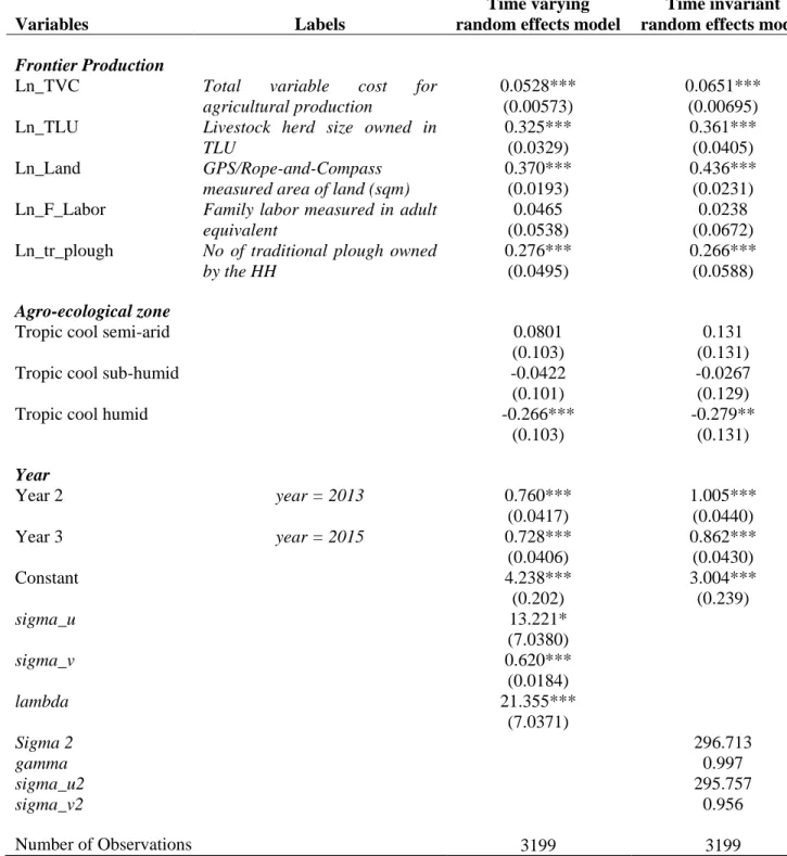
6.1 Frontier Production ... 19
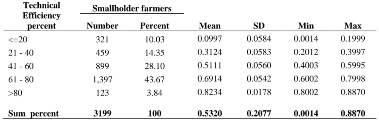
6.2 Technical Efficiency Estimates and Distribution ... 22
6.2.1 Technical Efficiency across Different Landholding and Livestock holding sizes ... 22
6.2.2 Technical efficiency across administrative regions and zones ... 23
6.3 Inefficiency Determinants ... 24
7. Conclusion and Recommendations ... 27
vi
8.1 Classification of Different Farming Systems and Agro-ecological Zones of Ethiopia ... 29
8.2 Overview of empirical studies on farmers’ technical efficiency, Ethiopia ... 30
8.3 The Maximum Likelihood Estimator (MLE) ... 32
8.4 National Data Summary Statistics ... 33
8.5 Descriptive statistics of data by region ... 34
8.6 Distribution of sample smallholder farmers across different regions and zones ... 38
8.7 Determinants of Technical Inefficiency and their Expected Signs ... 39
8.8 Baseline Econometric Analysis ... 41
8.8.1 Corrected Ordinary Least Square (COLS) Estimates using Pooled Data ... 41
8.8.2 Cross sectional data Analysis and Choice of Distributional assumption ... 43
8.9 Distribution of estimated technical efficiency scores ... 46
8.10 Distribution of Technical efficiency scores across different regions and zones ... 47
8.11 Regression result of the inefficiency model ... 48
vii
List of Figures
Figure 1. Technical and allocative Efficiency from an output orientation. (Source: Coelli, 1996). ... 9
Figure 2. Dataset creation process. ... 14
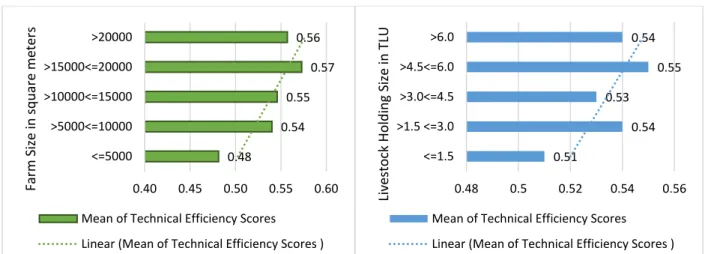
Figure 3. Distribution of technical efficiency across different (a) landholding and (b) livestock holding sizes. ... 23
Figure 4. Classification of (a) agro-ecological zones and (b) farming systems in Ethiopia.(source: Amede et al., 2017). ... 29
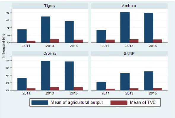
Figure 5. Annual average agricultural output and total variable cost among sample households, by region. ... 34
Figure 6. Annual average agricultural output and total variable cost among sample households, by region. ... 35
Figure 7. Distribution of number of sample smallholders by Region(i)_Zone(j). ... 38
Figure 8. Histogram of OLS residuals. ... 43
Figure 9. Distribution of estimated technical efficiency scores. ... 46
Figure 10. Distribution of predicted technical efficiency scores (in percent) by Region(i)_Zone(j). ... 47
List of Tables
Table 1. Households in crop productions and livestock activities by region ... 15Table 2. ML Estimate of Frontier Production. ... 21
Table 3. Mean and frequency distribution of technical efficiency. ... 22
Table 4. Regional mean technical efficiency. ... 23
Table 5. Overview of empirical studies of smallholder farm technical efficiency in Ethiopia. ... 30
Table 6. Descriptive Statistics of important variables, National. ... 33
Table 7. Descriptive Statistics of important variables, by Region. ... 37
Table 8. Inefficiency determinants and expected signs. ... 39
Table 9. OLS estimation of production function using log transformed variables. ... 42
Table 10. Cross-section SF models for year 2011, 2013 and 2015 (truncated normal). ... 44
viii
Acronyms
AGP Agricultural growth Program ATA Agricultural Transformation Agency
CD Cobb-Douglas
COLS Corrected Ordinary Least Square CPI Consumer Price Index
EA Enumeration Area
GDP Gross Domestic Product GLS Generalized Least Squares
GTP I(II) Growth and Transformation Plan I(II) HH(H) Household (Head)
ML(E) Maximum-Likelihood (Estimator)
MoFED Ethiopian Ministry of Finance and Economic Development1. NBE National bank of Ethiopia
OLS Ordinary Least Square
PASDEP A Plan for Accelerated and Sustained Development to End Poverty SFA Stochastic Frontier Approach
SDPRP Sustainable Development and Poverty Reduction Program USAID United States Agency for International Development
WB World Bank
WFP World Food Program
1
1.
Introduction
Why smallholders? Improving smallholders’ crop and livestock productivity is central not only to achieve increased yield and lead sustainable livelihood; but also contributes to poverty eradication and economic growth in such developing countries as Ethiopia. The livelihood of over 475 million smallholders, with total members of 3 billion people, is dependent on agriculture which represents 90 percent of the 570 million active farms in the world (Rapsomanikis, 2015; Abraham and Pingali, 2017). The importance of improving productivity of smallholder farming in the economic growth and poverty reduction has been recognized for years (Diao and Hazell 2004; Bahram and Chitemi 2006 and Diao et al., 2007). In fact, according to Timmer and Akkus (2008), very few exceptions of countries – Singapore and Hong Kong – have been able to ensure sustained decrease in poverty without increasing agricultural productivity.
Smallholder production – which serves as a primary source of income for 81 percent of the total population of Ethiopia – dominates agricultural production of the country (WB, 2016; USAID Feed the Future, 2016). The agriculture sector remains an important contributor to overall economic growth with about 40 and 90 percent shares to the GDP and exports (including coffee and chat2) respectively (Bachewe et al., 2015; and WB, 2017). The government of Ethiopia and international development partners recognized the role of smallholder agriculture as an important driver of economic development of the country (see e.g., ATA, 2018; AGP, 2018; and World Bank, 2007). As a result, the government of Ethiopia put smallholders farming at the heart of its policies. With a significant budget share to the agricultural sector, roughly seventeen percent of public expenditure, the Ethiopian development strategy supports one of the largest agricultural extension work force in the world (WB, 2016 and USAID Feed the Future, 2016).
How far to attain sustainable food security in Ethiopia? Despite rigorous works of the government of Ethiopia and development partners to improve smallholder agriculture, the rural livelihood in most parts of Ethiopia is still at its subsistence stage and highly dependent on erratic rainfalls. For example, according to Abduselam (2017), the number of people targeted as food insecure were 2.9 million in 2014, 4.5 million in mid-2015 and later at the end of the year this number grown to 10.2 million due to El Niño crisis. In late 2017, the government of Ethiopia and UN Office for the Coordination of Humanitarian Affairs (UNOCHA) identified 8.5 million people for emergency food aid (Tull, 2017). This number is in addition to eight million chronically food-insecure people who have been receiving food and cash support in the same year through the Government of Ethiopia-led Productive Safety Net Programme (PSNP)3 (Ibid.).
So what? Haji and Andersson (2007) noted that in developing agriculture based economies, where there is lack of resources and adoption of improved technologies is limited, efficiency plays an important role in increasing productivity growth. For this reason, investigation of smallholder farmers’ efficiency and hence efficiency determinants has substantial importance for economic development policy planning. According to Haji and Andersson (2007), an empirical examination of farmer's’ technical efficiency helps to: i) investigate the extent to which farmers utilize the existing technology, and ii) determine the scope of possibility to increase farmers’ technical efficiency without technological innovation. A wide array of applied work has been done to estimate Technical efficiency (TE) in agriculture using production frontier approach. A farmer’s technical efficiency measures the farmer’s ability to achieve the maximum possible agricultural output without changing the existing technology and using given set of inputs (Squires and
2Chat (Catha edulis Forsk ) is a mildly narcotic, stimulant perennial crop which is produced under an intensive production system
and young tender leaves and succulent twigs are chewed to gain mild excitement (Haji and Andersson, 2007 p.9).
3 Established in 2005, PSNP is aimed at enabling the rural poor facing chronic food insecurity to resist shocks, create assets and
2
Tabor, 1991). Technical efficiency of an individual farmer is measured based on his/her deviation, in terms of output, from the best-practice frontier or frontier production (Ibid.).
1.1
The Research Problem
This paper identified three gaps in the technical efficiency studies conducted in Ethiopia. First, to the researcher’s knowledge, little effort has been exerted to consider livestock production in studies regarding technical efficiencies of smallholding farmers in Ethiopia. The only exception is a technical efficiency study one by Haji and Andersson (2006), which included livestock production in whole-farm efficiency analysis. The major proportion of studies on technical efficiencies done in different parts of Ethiopia exclusively focused on crop production (Croppenstedt and Demeke, 1997; Admassie, 1999; Alemu et al., 2004; Alene and Zeller, 2005; Ahmed et al., 2013; Tirkaso, 2013; Seyoum et al., 1998; Alene and Hassan, 2003a; Geta
et al., 2013; Ahmed et al., 2014; all focused on either single or multiple crop production efficiencies). Nevertheless, investigation of smallholders’ efficiency wouldn’t be free from criticism of biasedness as long as no attempt is made in considering livestock production – which is a significant contributor for rural household economy. According to CSA and WB (2013, 15 and 17); 81.6 percent, 86.5 percent, and 87 percent of households have been practicing mixed farming (crop farming and livestock rearing) among sample rural households in the 2011, 2013, and 2015 waves ESS respectively. Technical efficiency studies of specialized farms would be reliable since inputs and outputs of production frontiers would be easily identified. In case of Ethiopian smallholders, where farm inputs cannot be easily allocated between crops and livestock production, it is not easy to get data with precise inputs division to estimate separate or sub-sector frontiers.
In order to have better understanding of crop-livestock farming, this paragraph describes a hypothetical example of a typical Ethiopian smallholding farmer operating on a mixed-farming system. Suppose a farmer has a small plot of land where she/he grows few types of crops on it. Draft animal power is used for transportation, tillage, cultivation, and threshing activities associated with crop production on this farm. Those animals at the same time are parts of inputs for livestock production either in the form of livestock (by)products per annum or annual gain in weights of animals. The land is used to produce edible crops and the crop residues will be saved and used as livestock feed throughout the year. Hence, this plot of land is technically used as an input for both crop production and livestock production indirectly. Household members divide their day time for crop production activities, looking after livestock, or doing both at the same time. Traditional plough and other farm tools can be considered as a capital in producing both crops and livestock feeds. Fertilizer cost is not only input for crop production, but also it contributes for increased quantity of feed production at the same time. Similarly, veterinary expenses are incurred to improve livestock health where crop production will also be positively affected as the healthier the animal the higher animal draft power is. Hence, almost all fixed and variable inputs including cattle, fertilizer, plough, and labor are jointly utilized towards increased total production. The proportion of ratio of sub-sectors’ production to the total farm output is not homogenous across smallholders.
In this scenario, no input can be considered as an exclusive input either for crop or livestock production. Depending on the weights of divisions of inputs between crop and livestock productions, keeping other factors constant, a farmer could be considered as less efficient in one of the sub-sectors while he is more technically efficient in whole-farm or other sub-sectors production. As far as smallholders’ economy is concerned, conclusions and policy recommendations only based on technical efficiency of single specialization would be misleading. Therefore, it is more appropriate to consider all inputs utilized for mixed-farming operations and estimate total annual farm outputs in investigating technical efficiencies and
3
identifying determinants of inefficiencies. Note: over nine-tenths of sample smallholder farmers included in this study are crop-livestock farmers and the remaining few have only either livestock or crop farms. Second, majority of technical efficiency researches in Ethiopia examined the influence of farm-specific, household characteristics, and socioeconomic factors on farm efficiencies. Environmental or geo variables, however, given less attention perhaps due to data limitation. Since smallholders’ agricultural production is highly dependent on environmental factors including of soil quality, topography, and climatic conditions, Sherlund et al. (2002) argues that environmental variables should be included in the estimation stochastic frontier. However, most technical efficiency studies fail to do so due to limited availability of data with detailed information on environmental production conditions (Sherlund et al., 2002; and Ogada et al., 2014). Sherlund et al. (2002) noted that the neglect of environmental variables leads to omitted variable bias and inaccurate estimates of technical efficiency scores. Thus, this study included agro-ecological variables in order to account for inter-farm heterogeneity in environmental production conditions such as soil quality, water, topography, and climatic conditions. Agro-ecological zonation is usually made based on agricultural and ecological features. According to Hurni (1998 p.1), each agro-ecological zone in Ethiopia has similar attributes in terms of: (i) agro-climatic conditions for crop farming and livestock rearing, (ii) land resource types such as soil, water or vegetative parameters, and (iii) topographical conditions. The map of Ethiopia with agro-ecological classification is presented in Appendix 8.1 Figure 4 (a). In addition, the farming system classification by Amede et al. (2017) indicates that farming systems differ from place to place mostly depending on which agro-ecological zone is the farmer located in (see Appendix 8.1 Figure 4 (b)). Thus, the inclusion of agro-ecological variable in the estimation of production frontier is assumed to capture for unobserved factors due to heterogeneity in several environmental production factors.
Third, only few technical efficiency papers appear to be done using panel data to estimate technical efficiency of Ethiopian smallholders. However, from econometric perspective, panel data is preferred to cross-section data because more accurate estimation of model parameters would be found when each individual is observed more than once (Thiam et al., 2001 p.237).
1.2
Research Objectives
General Research Question:
To what extent can total agricultural output be increased among sample smallholder farmers using the existing level of technology and given set of inputs and which factors influence this increment?
Purpose:
To determine the level of technical efficiencies of smallholders’ whole-farm production and examine the influence of different factors on and trends of estimated farm technical inefficiencies.
Specific objectives:
To estimate mean technical efficiencies of crop-livestock producers among smallholder farmers located in parts of major agricultural supplier regions of Ethiopia – Tigray, Amhara, Oromia, and SNNP4.
To examine the patterns of estimated level of technical efficiencies across regions, across different landholding and livestock holding sizes, and over years.
4
To investigate the effect of different inefficiency determinants on technical inefficiency of smallholders farmers under analysis
How? The present thesis utilizes stochastic frontier model in order to estimate technical efficiency of smallholders’ farm production; and identify determinants of the technical inefficiencies. Specifically, a random-effects (RE) time-variant method is employed using a panel data of smallholders across four major regions of Ethiopia. Household level farm efficiencies are estimated and mean technical efficiency is generated for the whole sample. The effect of demographic characters of households, location, and socioeconomic variables on technical inefficiency is evaluated. The patterns of level of farmers’ technical efficiency have been examined across different regions, different landholding and livestock holding sizes, and trends over years.
1.3
Significance of the study
This study is expected to be an important contributor for policy or intervention strategy designing by government line ministries and/or development organizations which are working to ensure improved livelihoods among smallholders in different parts of Ethiopia
.
As the study is focused at analyzing whole-farm technical efficiency of smallholders, it will be more representative to the household economy as compared to efficiency studies focused at sub-sector of farm economy.1.4
Organization of the Study
The rest of the thesis is organized as follows. Chapter two discusses the literature review. Chapter three presents important conceptual backgrounds to the econometric models. Chapter four explores methodology of the research in detail. Empirical results are discussed in Chapter five, while brief concluding remarks and policy recommendations are made in the last section. Finally, appendices and reference list are presented at the end consecutively.
5
2.
Literature review
The literature review section starts with the bigger picture of agriculture and analyses the two major contradicting opinions about the importance of agricultural productivity to sustainable economic development. Then, the role of smallholder agriculture is also analyzed in detail to have basic understanding about its significance to economic growth. Some selected papers on technical efficiencies of Ethiopian smallholder farmers are examined to get opportunities to make contributions to the literature by identifying gaps. Finally, different methods of panel data approach have been highlighted in order to grasp hints about the appropriate model among several options. It is important to note that comparison of specific results of this thesis and similar studies has been done in the results section, hence comparisons of specific findings are not included in this chapter in order to avoid repetition
2.1
Agricultural productivity and economic growth – different views
There has been opposing views on the role of agriculture productivity and consequent policy suggestions towards economic development. Dethier and Effenberger (2012) clearly noted that; i) agriculture has been a major preoccupation of international development organizations and governments of developing countries during the 1960s and 1970s; ii) later, in the 1980s and 1990s, agriculture has no more been a priority on development agenda; and iii) finally, agriculture reappeared in beginning of twenty-first century because of neglect and underinvestment.
Valdés and Foster (2010) concluded that most development literature in the mid-twenties is now considered as pessimistic in terms of the potential of agriculture for productivity and export growth. In the same vein, according to Hirschman (1958), most of development papers produced during that time demonstrated opinions that agriculture was not responsive to incentives and there were weak linkages with other sectors. In recent times as well, for example, Dercon (2009) argued that less attention should be given to agriculture and rather more efforts should be exerted in importing food and strengthening other sectors in order to ensure development (Dethier and Effenberger, 2012). Due to this set of misperceptions, agriculture has been neglected in search for policies that would boost economic development. For example, the share of agriculture in official development assistance (ODA) declined sharply from the maximum of eighteen percent in 1979 to 3.5 in 2004 (World Bank, 2007).
On the other hand, following Schultz (1964), development economists have been motivated in reconsidering efficiency of farmers and potential of the sector for sustainable economic growth (Valdés and Foster, 2010 p.1364). These studies indicated agriculture is sensitive to incentives and agriculture also has greater multiplier effect than it was perceived. Recognizing convincing successes in development, the 2008 World Development Report clearly marked that agriculture has not been used to its full potential in many countries because of anti-agriculture policy biases and underinvestment (see World Bank, 2007 p.44).Consequently, in recent years, developed countries and international development agencies have renewed their interest to make huge investment in agriculture (Dethier and Effenberger, 2012; and World Bank, 2007). For example, the Group of Eight (G8)5 countries promised to allocate 22 billion dollars for agricultural development during their meeting in Aquila, Italy in 2009 (Dethier and Effenberger, 2012).
Despite these varied narrations, opposing views regarding the role of agriculture to economic development do not necessarily contradict each other. The main reason for these differences is that development models have been derived under different economic assumptions (Dethier and Effenberger, 2012). Depending on
5 France, Germany, Italy, Japan, the United Kingdom, and the United States, Canada, and Russia were members of the G8 (see
6
the economic setup that a country has (e.g., openness to trade and being landlocked or not) and the position of agriculture in a country’s economy, the role of agriculture to development will have a different outlook among countries and thus different country-specific policies need to be developed. Mellor and Johnston (1961) underscored policies should take account of the phases of agricultural development and its implication. Similarly, Heady et al. (1965) stressed adjustments should be made to agriculture and be consistent with the stage of economic development. Agro-pessimists also admit that agriculture can significantly contribute to economic development under certain circumstances (Dethier and Effenberger, 2012). For example, they mentioned that agriculture should be supported to stimulate overall economic growth if a country is landlocked and has a closed economy model. Hence, “tailor-made” or country- and case-specific development programs are needed to make sure that agriculture is in a better position for long-run economic benefits.
Now let us narrow the issue down to the case of smallholders who virtually represent agriculture in developing countries. Approximately 90 percent of the 570 million farms in the world are operated by 475 million farm households with a total member of three billion people (Rapsomanikis, 2015; Abraham and Pingali, 2017). In the case of developing countries, agricultural growth in comparison to the non-agricultural growth will favor the poorest in terms of increase in income – meaning better in reducing income inequalities (Valdés and Foster, 2010). On the other hand, according to Collier and Dercon (2014), it has been argued that growth in the agricultural sector is dependent on the demand which is driven by the non-agricultural parts of the economy. However, for certain landlocked economies in Africa with difficult relations with their neighbors, such as Ethiopia, it is reasonable to assume agricultural production will have to lead the growth process (Ibid.). For example, a cross-country panel data analysis by Bravo-Ortega and Lederman (2005) indicated that increase in agricultural income raises nonagricultural GDP in developing countries, while the reverse relation exists for developed countries (Dethier and Effenberger, 2012). Regarding poverty, evidence show agricultural growth in developing countries has relatively greater importance in poverty reduction than other sectors (e.g., World Bank, 2007).
2.2
Empirical Evidence on Smallholder Farmers’ Technical Efficiencies
in Ethiopia
Beyond ensuring a sustainable food supply, investigation of smallholders’ farm efficiency and hence efficiency determinants are of substantial policy relevance for economic development. Haji and Andersson (2006) and Sherlund et al. (2002) noted in developing agriculture-based economies, where there is lack of resources and the adoption of improved technologies is limited, efficiency improvements play a significant role in achieving economic growth. Thus, precise estimation of efficiency scores and analysis of inefficiency determinants is quite important for public investments focused at increasing farmers’ productivity (Sherlund
et al., 2002).
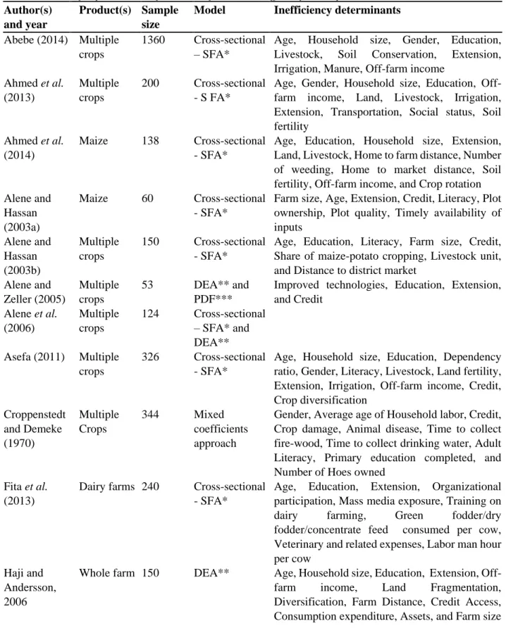
Table 1 (see Appendix 8.2) presents a brief description of some selected papers focusing on investigating technical efficiency of smallholder farmers in different parts of Ethiopia. As indicated, a total of sixteen papers are included in the list out of which ten studies are done on multiple crop production, three on maize production, two on dairy farms, and only one study has been conducted on whole farm efficiency. As shown in Table 1 (Appendix 8.2), most of the papers employed stochastic frontier approach (SFA) using cross-sectional (twelve papers). Only one paper is presented for each of the following models – data envelopment analysis (DEA), DEA and SFA with cross-sectional data, DEA and parametric distance function (PDF), and mixed fixed-random coefficients approach.
7
In general, a major subset of technical efficiency studies done for the last two decades in Ethiopia are mainly focused on either multiple crop production or a single crop production technical efficiency. For example, Croppenstedt and Demeke (1997), Admassie (1999), Alemu et al. (2004), Alene and Zeller (2005), Ahmed
et al. (2013), and Tirkaso (2013) studied technical efficiency of multiple crop production and associated inefficiency determinants. Seyoum et al. (1998), Alene and Hassan (2003a), Geta et al. (2013), and Ahmed
et al. (2014) examined technical efficiency of maize production and its determinants. Fita et al. (2013) estimated technical efficiency scores of dairy production. Likewise, Haji and Anderson (2007) studied technical efficiency of whole-farm and vegetable production and determinants of inefficiencies. Relatively, limited efforts were exerted to study technical efficiencies of farms specializing in livestock and dairy and those viewed as a whole (i.e. mixed farms).
It seems almost no one considered livestock production in studies regarding technical efficiencies of smallholding farmers in Ethiopia. The only exception to this is a research done by Haji and Andersson (2006) estimated vegetable as well as whole-farm (both crop and livestock production) efficiency in two districts. Similarly, apart from Ethiopia, the proportion of studies done globally on multiple or single crop production and dairy farm efficiencies is significantly higher than that of studies done on whole-farm efficiency. Technical efficiency studies done on cattle or livestock farming are somewhat sparse. For example, out of 167 published papers included in a meta-regression analysis done by Bravo-Ureta et al.
(2007), only one study was done on livestock technical efficiency following the second least category – other animals (six). In the aforementioned meta-regression analysis, crops (either multiple or single crop) is the dominant category with 109 studies, followed by dairy and cattle (46), and whole farm (23). In countries like Ethiopia, the role of livestock in the economy is quite significant and hence technical efficiency study in the livestock sector would be equally important.
In mixed crop-livestock system, livestock is the second major source of household income (FAO, 2018). Likewise, at national level, the mixed crop-livestock systems contribute to a significant share, two-thirds, to the total net income (Ibid.). The crop-livestock system is concentrated in the mid- and high-altitude, where the major agricultural production comes from. As crop-livestock systems are technically very interlinked, one can hardly separate production inputs for each activity. In this case, it would be very difficult to get accurate estimates of technical efficiency and analysis of corresponding determinants if we consider sub-sector efficiency analysis of farms. The problem with input allocation, especially when one deals with national or regional level data, is that utilized multiple inputs cannot be easily broken down into crop and livestock sectors (Alene et al., 2006. p.53). Due to this problem, studies conducted in sub-sector productivity – such as Rae and Hertel (2000) – were based on highly imperfect, partial factor productivity measures (Alene et al., 2006. p.53). For this reason, instead of sub-sector efficiency analysis, the best alternative would be to utilize a single production frontier approach using aggregated value of all farm outputs by considering all agricultural inputs utilized.
The challenge of quantifying the annual value of production gained from livestock would be the main reason for not considering livestock production in smallholders’ technical efficiency studies in Ethiopia. Likewise, estimating the amount or value of livestock feed utilized during the year is not as easy as those of the commercial farms. Commercial farms usually have records of the cost or quantity of livestock feed utilized whereas smallholders commonly use crop residues and/or free grazing to feed their livestock. Bagi and Huang (1983) estimated production technical efficiency of farms including 115 crop farms and 78 mixed-farms. In the case of mixed-farms, in addition to total value of crop output, they included the “value added” to livestock over the year and the income from actual livestock sales during the year in calculating the total output. Likewise, while calculating total mixed-farm outputs, this thesis included; i) the monetary value of crop outputs, and ii) income from actual sales of live animals, iii) income from sales of livestock products
8
and livestock byproducts if any. Due to data limitation, the value of annual increase in herd size is not included in calculation of annual total farm outputs. Nonetheless, herd size among Ethiopian smallholders is strongly and positively associated with household’s choice of participation on cattle market as a seller (Negassa and Jabbar, 2008). They also noted that for farm households in the predominantly crop–livestock systems, livestock births account the majority of inflows to the livestock herds and flocks. Similarly, livestock sale represents the major share of outflows from the livestock herd and flocks. Meaning, households with larger herd size have higher ability to generate surplus animals and are therefore more likely to sell live animals. Though the total number of livestock in Ethiopia is the largest in Africa, the number of livestock at the level of the individual smallholder farmers and remains very low (SA et al.,
2012).This implies that smallholders tend to keep more or less equivalent herd or flock sizes or at least no significant changes be made within a year. Hence, the value of increase in herd side can significantly be captured by the sale of live animals. For this reason, this study does not include the increase in herd size in calculating the total value of annual agricultural output.
Another dimension this thesis tries to take advantage of it is that most studies on technical efficiencies done in Ethiopia did not account for agro-ecological factors, probably due to unavailability of data. None of the papers listed in Table 1 (Appendix 8.2) included environmental or agro-ecological production conditions. Ignoring such factors cost a lot in terms biased parameter estimation and variations due to these factors will be regarded as real efficiency differences (see e.g., Ogada et al., 2014; and Liu and Zhuang, 2000). Salami
et al. (2010) showed smallholders can be categorized on the basis of the agro-ecological zones in which they operate for more precise policy designing and implementation. Thus, for accurate results, this thesis incorporated agro-ecological zones (as dummy variables) in order to account for uncontrolled location-specific climate factors.
2.3
Panel Data Models in Technical Efficiency Studies
Based on the data type they use, econometric estimation of stochastic production frontiers can be categorized as cross-section or panel data models. Model (4) is a stochastic frontier production function defined for cross-sectional data where each household is observed once at a particular time. If households (farmers) in the sample are observed at several times over time, then the data are referred to as panel data. Schmidt and Sickles (1984) pointed out major limitations associated cross-section studies: i) inconsistent estimates of a particular firm technical (in)efficiency; ii) estimation of the model and separation of the inefficiency from the statistical noise requires specific distributional assumption (e.g., half-normal or exponential); iii) it may not be correct to assume that inefficiency is independent of regressors. Panel data model solves all these problems because one can take into account some heterogeneity and some rigidities or limitations can be removed (Schmidt and Sickles, 1984; Thiam et al., 2001; Murillo‐Zamorano, 2004; and Battese and Coelli, 1995). Moreover, from an econometric perspective, panel data is preferred to cross-section data because more accurate estimation of model parameters would be found when each individual is observed more than once (Thiam et al., 2001, p.237).
Nevertheless, a significant share of farm technical efficiency studies in Ethiopia employed cross-section data probably due to data limitations (e.g., Abebe, 2014; Ahmed et al., 2013; Tirkaso, 2013; Asefa, S., 2011; Wubeneh and Ehui, 2006; Alene et al., 2006; Haji and Andersson, 2006; and Seyoum et al.,1998). There are few exceptions which used panel data analysis (e.g., Demeke et al., 2011). Understandably, one of the gaps this thesis is supposed to fill is that most technical efficiency studies in Ethiopia do not utilize panel data.
9
3.
Conceptual background
This section explains the conceptual models used for analyses and alternative models which are not considered in this study. The discussion starts with the wider concept, economic efficiency, where basic economic background to technical and allocative efficiency is provided. Several production frontier approaches are also discussed and justification for selecting stochastic frontier approach is provided. Moreover, the specific model selected for this study, time-variant random effects model, is explained in detail and its advantage over other alternative methods is also provided.
3.1
Economic efficiency and its components
In his well-known paper, Farrell (1957) categorized efficiency of a firm into two components: technical efficiency – the ability of a firm to obtain the maximum attainable output available from a determined set of inputs, and allocative efficiency – the ability of a firm to use optimal package of inputs given their prices and marginal productivities. Economic efficiency, therefore, can be defined as a well-specified output at minimum cost6. Two important questions could arise in relation to economic efficiency: (i) “to what amount
can factor inputs proportionally be reduced without affecting a given level of output?” and (ii) to what extent can output level be proportionally expanded without altering a given set of inputs?” Farrell addressed these two questions through input-oriented and output-oriented efficiency measures respectively.
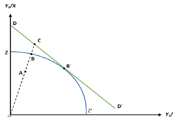
For a better understanding of economic or overall efficiency and its components, Farrell’s analysis of output-oriented measures of efficiency was illustrated by Coelli (1996) as shown in Figure 1. Consider a case where production involves two outputs (Y1 and Y2) and a single input X.
Figure 1. Technical and allocative Efficiency from an output orientation. (Source: Coelli, 1996).
6 Farrell (1957) termed price efficiency and overall efficiency instead of latter literature terminologies of allocative efficiency and
10
For simplicity, one can assume constant returns to scale (CRS) therefore technology can be represented by a unit production possibility curve XX' in two dimensions. The curve ZZ' is the unit production possibility curve, i.e. it represents the upper bound of production possibilities. Such firms operating below the ZZ' curve as the one which operates at point A are therefore inefficient. Hence, the distance AB along the ray OC' represents technical inefficiency of a firm operating at point A, meaning output could be increased without requiring additional input. Geometrically, technical inefficiency of the firm operating at point A can be expressed by the ratio AB/OB. Hence, the technical efficiency (TE) of the firm under analysis (1-AB)/OB would be given by the ration of OA/OB.
Assuming market price is given and a particular behavioral objective such as revenue maximization is assumed in such a way that the output price ratio is reflected by the slope of isorevenue line DD'; allocative efficiency of the firm under study can also be derived from the unit isoresource plotted in Figure 1. Hence, the focus will now be on the distance given by the line segment BC along the array OC, which in relative terms could be given as BC/OC. The maximum attainable revenue with the given level of input is given by point B'. Therefore, the ratio BC/OC indicates that the revenue expansion that a firm would be able to achieve if it moved from a technically efficient output combination (point B) to a both technically and allocatively efficient one (point B'). This indicates that the allocative efficiency of a firm operating at point A is given by OB/OC.
The measure of what Farrell (1957) termed overall efficiency and later literature has renamed economic efficiency (EE) can be derived from the multiplicative interaction of both technical and allocative components; 𝑻𝑬 =𝑂𝐴 𝑂𝐵 𝑎𝑛𝑑 𝑨𝑬 = 𝑂𝐵 𝑂𝐶 (1) 𝑬𝑬 = 𝑇𝐸 × 𝐴𝐸 = 𝑂𝐴 𝑂𝐵 × 𝑂𝐵 𝑂𝐶 = 𝑶𝑨 𝑶𝑪 (2)
where the distance involved in its definition (AC) can also be analyzed in terms of revenue expansion. The output-oriented efficiency analysis of Farrell (1957) is described in this section in order to have better understanding about economic efficiency and its components – technical and allocative efficiency. A thorough analysis of input-oriented efficiency measures can be found in Murillo‐Zamorano (2004) and Coelli (1996). It is worth to mention here that under the assumption of CRS, input-oriented and output-oriented measures of technical efficiency are equivalent (Färe and Lovell, 1978).
3.2
Production frontier approaches
In microeconomic theory a production function (or frontier) is defined in terms of the maximum output that can be produced from a determined package of inputs given the existing technology. A large number of frontier models developed based on Farrell’s original work in 1957 can be classified into two major categories – parametric and non-parametric (Thiam et al., 2001). Non-parametric TE models, often referred to as Data Envelopment Analysis (DEA), are based on mathematical programing techniques. Unlike the parametric models, DEA neither imposes any functional form nor makes assumptions about the error terms. Though DEA is free from misspecification, it is not preferred for analysis in this thesis due mainly to its failure to account for measurement errors and other sources of statistical noise. Thus, as all deviations from the frontier are assumed to be the resulted from technical inefficiency, real efficiency scores may be under estimated (Hansson Öhlmér, 2008).
11
Parametric models can either be non-stochastic or stochastic. As Murillo‐Zamorano (2004) explained, the non-stochastic econometric approach enables analysts to estimate rather than ‘calculate’ the parameters of the function by adopting the technological framework introduced in the mathematical programming model, i.e. statistical inference will be possible based on those estimates. Nevertheless, alike to DEA, a problem with non-stochastic frontiers is that no account is taken of statistical noise, and hence any deviation from the frontier is assumed to be caused by inefficiency.
Due mainly to their failure to provide accurate measures of productive structure (Murillo‐Zamorano, 2004), goal programming models or non-stochastic econometric approaches are not used in this study. In the next section, a detailed analysis of an alternative econometric approach, stochastic frontier models, is provided.
3.3
Stochastic Frontier Models
As noted by Murillo‐Zamorano (2004), an obvious solution to the problem associated with non-parametric and non-stochastic frontier approaches is to introduce a double-sided random error into the frontier model specification. The resulting frontier is known as stochastic frontier – where both specification failures and uncontrollable factors are modeled independently of the inefficiency component. Stochastic frontier model was independently developed by Aigner, Lovell and Schmidt (1977), and Meeusen and Van den Broeck (1977), and it can be written as:
𝑌𝑖= 𝑓(𝑥𝑖; 𝛽) exp(𝑣𝑖− 𝑢𝑖) 𝑖 = 1, 2, … , 𝑁 (3)
where 𝑌𝑖 represents the total possible maximum output of the ith firm (farmer), 𝑥𝑖 a vector of 𝑁 (farm) inputs,
𝑓(𝑥𝑖; 𝛽) is a suitable production frontier (it can take Cobb-Douglas or TRANSLOG functional form) which depends on inputs and a vector of technological parameter β. The term 𝑣𝑖− 𝑢𝑖 can be decomposed into 𝑣𝑖
– which represents statistical noise (the regular error term) and 𝑢𝑖 – which represents technical inefficiency, meaning the deviation of output from the frontier for each individual firm (farm). The output-oriented measure of technical efficiency of a firm can be defined as the ratio of its observed output, 𝑌𝑖, to the stochastic to the corresponding stochastic output:
𝑇𝐸𝑖 = 𝑌𝑖
𝑓(𝑥𝑖; 𝛽) exp(𝑣𝑖)=
𝑓(𝑥𝑖; 𝛽) 𝑒𝑥𝑝(𝑣𝑖−𝑢𝑖)
𝑓(𝑥𝑖; 𝛽) 𝑒𝑥𝑝(𝑣𝑖) = 𝑒𝑥𝑝(−𝑢𝑖
) (4)
Technical efficiency of the 𝑖𝑡ℎ firm, 𝑇𝐸𝑖, takes a value between zero and one and it will be predicted once the parameters of the stochastic frontier (i.e. model (4)) are estimated.The statistical noise, 𝑣𝑖, is assumed to be identically independent and identically distributed. For the one-sided error (inefficiency), 𝑢𝑖, half-normal, exponential, exponential, and truncated-normal distributional assumptions have been frequently assumed used in the literature7. Under the assumption that the two error terms are independently distributed from each other and from the regressors, Maximum Likelihood estimates can be determined. A brief description of Maximum Likelihood Estimator (MLE) is provided in Appendix 8.3.
3.4
Time-Variant Model
Stochastic frontier panel data models can be either time-variant or time-invariant, mainly depending on their assumption about inefficiency over time8. The time-variant model assumes that inefficiency effects are firm-specific and time-varying. In the time-invariant model, inefficiency term is assumed to be firm-firm-specific and
7 A detail review of the half-normal, exponential, gamma, and truncated-normal distributional assumptions can be found in
Murillo‐Zamorano (2004).
12
time-invariant. As the time period of panel data becomes large, it is not realistic to assume that inefficiency level of a given firm does not change over time (Coelli, 1995). Kumbhakar et al. (2015) and Coelli (1995) suggested that time-invariant model can be employed for short time panel data models, where inefficiency determinants are not expected to change during time period of the study (Kumbhakar et al., 2015; Coelli, 1995). However, based on the summary statistics of important variables from the data employed in this thesis, there are noticeable changes in output per specific inputs over years, which implies that productivity is changing over years whatever the magnitude of the change is. In fact, reports from development programs or agencies show that smallholders’ productivity has been increasing over years (see e.g., ATA, 2018; AGP, 2018, World Bank, 2017). This indicates smallholders productivity growth, and hence efficiency, are expected to be improved during the period the data was collected. For this specific study, the time-variant model is well justified as at least very small difference is expected in level technical efficiency of smallholder farms over years.
Based on model (4), panel data model (i.e. Cobb-Douglas Production function) can be can be presented as follows,
𝑦𝑖𝑡 = 𝛼 + 𝑥𝑖𝑡′𝛽 + 𝑣𝑖𝑡− 𝑢𝑖𝑡 𝑖 = 1, … , 𝑁, 𝑡 = 1, … , 𝑇. (5)
Here, the subscripts 𝑖 and 𝑡 index the farm households and time periods respectively. 𝑦𝑖𝑡 represents the total output of the 𝑖𝑡ℎ farm household at time 𝑡, whereas 𝑥𝑖𝑡 is a vector of farm inputs utilized by the 𝑖𝑡ℎ farm household at time 𝑡. The 𝑣𝑖𝑡 is statistical noise and uncorrelated with regressors. The 𝑢𝑖𝑡 is technical
inefficiency of the 𝑖𝑡ℎ farm household at time t, and correspondingly, 𝑢
𝑖𝑡 ≥ 0 for all 𝑖.
Based on the time-variant model, one can assume 𝑢𝑖 as a fixed – fixed-effects model or random parameter – random-effects model. Since these models do not impose any distributional assumption on 𝑢𝑖, they are referred as distribution-free approaches. The Fixed effects model assumes that 𝑢𝑖 is allowed to be freely correlated with the regressors, which is may be a desirable property (Kumbhakar et al., 2015). However, this models have a limitation that time-invariant attributes of the households could cause multicollinearity problem. Kokkinou (2010) also noted that fixed-effects model could provide unrealistic technical efficiency scores due to poor estimation of parameters of frontier production. Thus, the random effects model is selected for this study because the time-invariant variables, such as gender, region, and agro-ecological zones can be included as regressors without the problem of perfect multicollinearity.
The random-effects model can be estimated either by generalized least squares (GLS) or using the maximum likelihood (ML) method (see e.g., Kumbhakar et al., 2015; and Schmidt and Sickles, 1984). Schmidt and Sickles (1984) noted that, as 𝑁 → ∞ regardless of 𝑇, MLE’s are consistent and asymptotically efficient than the GLS estimator. Using ML estimator, it is possible to impose distributional assumptions on the error terms and their independence on the regressors (Schmidt and Sickles, 1984). A brief discussion of MLE and corresponding mathematical derivations are presented in Appendix 8.3.
13
4.
Data
4.1
Smallholder agriculture in Ethiopia
Ethiopia, Africa’s second most populous country, has achieved substantial economic development over the past decade envisioning to be a middle income country by 2025 (WB, 2017)9. The country has a population of 97 million people and a land size of 1.14 million square kilometers (WFP, 2018 and NBE, 2017). Agriculture, virtually represented by smallholders farming, has been a major pillar of the economy and remained to be the primary focus of development agendas towards the country’s vision of becoming a middle income country (WB, 2016; USAID Feed the Future, 2016). The sector remains an important contributor to overall economic growth with about 40 percent and over 90 percent shares to the GDP and exports (including coffee and chat10), respectively (Bachewe et al., 2015; WB, 2017).
Cereals, pulses and oilseeds altogether categorized as grain crops, constitute the major food crops for the majority of the country’s population and also contribute significantly to the household income as well as foreign currency earnings (CSA, 2017). According to CSA (2017)’s main production season post-harvest crop production survey, a total of 12,574,107.33 hectares of land were covered by grain crops with a corresponding total grain yield amounting 290,385,593.21 quintals. Ethiopia has the largest livestock population and the highest draft animal population in the continent (Solomon et al., 2013 p.2). There are approximately 59.5 million cattle, 60.9 million sheep and goats, 11 million equines (including horses, mules and donkeys), 59.5 poultry, 2.4 million camels and 6.2 million beehives (CSA, 2017).
The government of Ethiopia and international development partners recognized the role of smallholder agriculture as an important driver of economic development of the country (see e.g., ATA, 2018; AGP, 2018; and World Bank, 2007). The agricultural sector exhibited 6.7 percent growth rate in 2016/17, becoming the major source of the 10.9 percent GDP growth rate in the same year (NBE, 2017). The Ethiopian government, in its Growth and Transformation Plan (GTP), and the World Bank, in its Country Partnership Framework for Ethiopia, clearly stated that sustainable economic growth will be attained through smallholders’ productivity (MoFED, 2014; and World Bank, 2017). Ethiopian government – in collaboration with international development organizations – has been implementing long-term country-led programs aiming at increasing production and productivity of smallholder production (WB, 2016; USAID Feed the Future, 2016). For example, Sustainable Development and Poverty Reduction Program (SDPRP)11, Plan for Accelerated and Sustained Development to End Poverty (PASDEP)12, and Growth and Transformation Plan I (GTP I) have been successively implemented from 2003 through 2015 (MoFED, 2002, 2006, and 2014). Smallholding agriculture was the top priority in all of these national level economic strategies. Growth and Transformation Plan II (GTP II)13, a continuation of GTP I, is currently (2016 - 2020) under implementation with the notion that agriculture will remain key driver of economic growth (World Bank, 2017).
9 Report No. 115135-ET.
10Chat (Catha edulis Forsk ) is a mildly narcotic, stimulant perennial crop which is produced under an intensive production system
and young tender leaves and succulent twigs are chewed to gain mild excitement (Haji and Andersson, 2007 p.9).
11 SDPRP, a three years national level development strategy (2003 – 2005), had the following major focus areas: overriding primacy
to smallholders’ development, private sector growth and encourage investment, increased commodity export mainly agricultural products, investment on education, strengthen administrative decentralization, governance improvements, promoting agricultural research, and increased water resources utilization (see MoFED, 2002).
12 PASDEP has been implemented for five years (2006 – 2010) with the following eight major pillar: capacity building, massive
push towards speeding up growth mainly by greater commercialization of agriculture, balancing economic development with population growth, women empowerment, infrastructure development, development of human resource, able to manage risk and volatility, and reducing unemployment (see MoFED, 2006).
13 GTP II intends a 20 percent increase in agricultural output by smallholders’ living in the rural areas and ensure sustainable food
14
4.2
Data Source and Data Processing
The Ethiopian Socioeconomic Surveys (ESS)
This thesis utilized a panel data created using the ESS, which were implemented by the Central Statistics (CSA) of Ethiopia and the World Bank’s Living Standards Measurement Study (LSMS) team. According to (CSA and WB, 2013, 15, 17), ESS has been implemented in three rounds – in 2011, 2013 and 2015. The surveys were done in representative rural and small town areas of Ethiopia on a range of household community level characteristics linked to agricultural activities. The same households, with a rich set of information on agriculture, food security, shocks, demography, education, health, savings, labor, and welfare, are observed over three years. Data from all the three waves is freely availed by World Bank14.
Data Processing
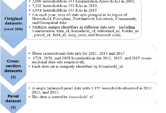
The data processing (data cleaning) was tricky and took considerable time before proceeding with the econometric analysis. The reason for this stems from the fact that the ESS data covers a wide range of topics and includes multiple data sets (over 200 data files). Hence, one has to go through several data sets to get relevant information in order to create a database of sampled farms from the ESS with all relevant variables. In addition, there is no common identifier across all data sets which makes the creation of a single data set more difficult. A thorough processing of the data which involved multiple stages of tasks, has been done to produce three cross-sectional data sets where each of them were sorted by household id15. As illustrated in
figure 2, a balanced panel data consisting of 3,465 observations (1155 households) is created with a time series of three years. The data processing work as well as the analysis part is done using STATA program.
Figure 2. Dataset creation process.
14 More information about and data from the Ethiopian Socioeconomic Surveys (ESS) of wave 1 – 3 done in 2011, 2013 and 2015
can be found at the World Bank’s website – in the Living Standards Measurement Study (LSMS) category of Central Microdata Catalog: http://microdata.worldbank.org/index.php/catalog/lsms.
15
4.3
Descriptive Statistics
The study considers data only from four major regions of Ethiopia – Tigray, Amhara, Oromia and SNNP regions. The exclusive focus on these four regions is due mainly to – i) the ERSS sample is representative for these regions, ii) over 90 percent of the country’s population lives in these four regions; and iii) enormous production levels of agricultural outputs, for example, in the 2016/17 main agricultural production season, these four regions represented 97 percent of area of grain crop land, 97 percent of grain crop yield, 93 percent of total livestock population (in TLU), and 94 percent of total number of beehives in Ethiopia (CSA and WB, 2013 and 2017). Table 1 illustrates the distribution of sample smallholders across regions and farm specializations.
Table 1. Households in crop productions and livestock activities by region
Region
Number of households
District (woredas)
percent of HHs by Type of Farm by region
Crop Livestock Mixed Tigray 151 9 11 4 85 Amhara 349 17 9 1 90 Oromia 247 17 6 2 92 SNNP 410 13 5 0 95 Total 1157 56 7 1 92 Source: CSA (2013, 15, 17)
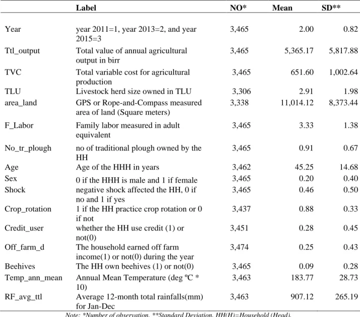
The panel data consists of 3,465 observations (1,155 households) spread over three years (2011, 2013 and 2015). The average value of agricultural outputs is ETB 5,365.17 per annum (See Table 6 in Appendix 8.4). The corresponding standard deviation is ETB 5,817.88, which is an indication of significant variability in the value of agricultural output among households under study. Similarly, as indicated in Table 6, a similar pattern is also observed for total variable costs and average livestock herd size. The average land size owned by sample households is approximately 1.1 hectares at national level. The average family labor (in adult equivalent) and number of traditional ploughs owned by households is 3.33 and 0.91 respectively.
As presented in Table 6 (Appendix 8.4), the average age of household heads under study is 45.25 years. Twenty percent of the sample household heads are female while the remaining sixty percent households are male headed. As indicated, 46 percent of sample households were negatively affected by shocks which includes death of family member (mainly bread earner), flood, drought, etc. A quarter of sample households have been involved in off-farm activities. It is also shown that around an average of 28 percent of target households have received credit in each year. Majority of the households under study practice crop rotation, 88 percent. On average 9 percent of the sample households own at least one beehive.
Moreover, as the study also focuses on examining the regional patterns of technical efficiency scores, it is reasonable to provide detail analysis based on regional level descriptive statistics. In Appendix 8.5, a detail illustration of summary statistics of regional level data is provided in order to be able to see how variables behave across regions.
16
5.
Empirical Strategy
The Econometric Specification
In agricultural economics literature, different functional forms (e.g., Cobb-Douglas and translong) are usually used to estimate agricultural production frontiers. Researches on developing countries technical efficiency have mostly used Cobb-Douglas functional form, though it has been generally concluded that choice of functional form does not affect the technical efficiency scores (Thiam et al., 2001).
Following Battese and Coelli (1995), a stochastic frontier production for panel data is presented (i.e. Cobb-Douglas functional form for simplicity of estimation and interpretation of parameters):
𝑌𝑖𝑡 = 𝑓(𝑥𝑖𝑡; 𝛽) exp(𝑣𝑖𝑡− 𝑢𝑖𝑡) 𝑖 = 1, 2, … , 𝑁 𝑡 = 1, … , 𝑇 (15) where the technical inefficiency term is identified as
𝑢𝑖𝑡 = 𝑓(𝑧𝑖𝑡; 𝛿) 𝑖 = 1, 2, … , 𝑁 𝑡 = 1, … , 𝑇
where: 𝑌𝑖𝑡: is output at time 𝑡 by the 𝑖𝑡ℎ farmer;
𝑥𝑖𝑡: (1×k) vector of inputs to produce output Y
𝛽: (k×1) vector of unknown parameters
𝑣𝑖𝑡: random errors independently distributed of the 𝑢𝑖𝑡𝑠
𝑢𝑖𝑡: non-negative random variables associated with technical inefficiency of production
𝑧𝑖𝑡: (1×m) vector of explanatory variables associated with the technical inefficiency
𝛿: (m×1) vector of unknown coefficients of the inefficiency model The production frontier is specified as;
𝑇𝑜𝑢𝑡𝑝𝑢𝑡 = (𝐿𝑎𝑛𝑑, 𝑇𝐿𝑈, 𝑇𝑉𝐶, 𝐹𝐿𝑎𝑏𝑜𝑟, 𝐴𝑔𝑟𝑜𝑒𝑐𝑜𝑙𝑜𝑔𝑦, 𝑌𝑒𝑎𝑟 )16
Real value
In order to account for price inflation, GDP deflator – with 2010 base year price – has been used to calculate the real monetary values of different agricultural (by)products and inputs utilized using data from the IMF’s website17. GDP deflator is used because it provides comprehensive measure of inflation as it covers all goods and services in the economy, whereas data on Consumer Price Index (CPI) considers a specific basket of goods and services.
The dependent variable, 𝑻𝒐𝒖𝒕𝒑𝒖𝒕
𝑇𝑜𝑢𝑡𝑝𝑢𝑡: = the estimate of total monetary value (i.e. in ETB18) of agricultural products by a given farm household in year 𝑡. The total value of farm output included crop output, sale of live animals, and sale of livestock (by)products (all in monetary term). The monetary value of total crop output by a given farm household is an aggregation of all types of crop (in monetary term) produced by the household. The calculation is done using a zonal (mostly), regional, or national level crop-specific prices upon availability data. The livestock sale, if a farmer has sold any in year 𝑡, is the revenue earned from sale of any type of live animals
16 The identification of output and input variables in crop and livestock production satisfies the basic properties of production
function. Production function has basic properties of non-negativity, weak essentiality, non-decreasing in x, and concave in x. These properties, however, are neither exhaustive nor universally maintain. (see e.g., Coelli et al., 2005).
17http://www.imf.org/external/datamapper/datasets
18 ETB stands for Ethiopian Birr – a national currency of Ethiopia. currently 1USD = 27.92 ETB (based on exchange rate available
17
including, cattle, sheep, goats, horses, donkeys, mules, and chicken. Sale of Livestock (by)product is the revenue earned by a given farmer from actual sale of livestock (by)product including, eggs, honey, milk and milk products, meat, and animal skin. The income from livestock and livestock (by)products is calculated using the method of the FAO Rural Livelihoods Information System (RuLIS)19. The only difference with the RuLIS is that the current aggregation didn’t consider the value of self-consumed livestock (by)products due to data unavailability.
Production Inputs, vector of 𝒙𝒊𝒕 and expected signs
As clearly discussed in section 1.1, a single stochastic frontier is chosen instead of sub-sector efficiency analysis methods in order to make sure that the model is not suffering from omitted variable bias or to avoid errors in identifying the inputs with the right amount for the sub-sector production. In this model, all farm inputs are included using appropriate units. The following input variables are used for the whole-farm production of a given farm household;
𝐿𝑎𝑛𝑑: = area of land owned by the household in square meters. Land is used to grow different crops and crop residues are used for livestock feeding. Land is expected to have a positive sign as in (e.g., Bagi and Huang, 1983; Tirkaso, 2013)
𝑇𝐿𝑈: = total number of livestock owned by the household are included. This includes virtually all categories of livestock which are common to Ethiopian smallholders except camel (camels are mostly found in the pastoralist area). Cattle, small ruminants (sheep and goats), non-ruminant grazing animals (donkeys, mules, and horses) and chickens are included in the study. In order to have a common unit of measurement, TLU20 (Tropical Livestock Units) has been used to aggregate total livestock herd size owned. TLU is expected to have a positive sign in the production function.
𝑇𝑉𝐶: = total variable cost (in monetary terms – ETB) incurred by a given farm household for crop and livestock production in year 𝑡. TVC includes, cost of fertilizer, veternary expenses, and other miscellaneous expenses. TVC is also expected to positively correlated with the dependent variable, 𝑇𝑜𝑢𝑡𝑝𝑢𝑡.
𝐹𝑙𝑎𝑏𝑜𝑟: = family labor – number of adult members of a given farm household in year 𝑡. Family labor is measured in terms of adult equivalent21.
Control Variables
Control variables are included in order to capture variations in output and inputs due to due to different agro-ecological characteristics of locations of sample smallholder farmers and weather condition variations over years. Agro-ecological zones are categorized into four major groups in order to control for differences due to several environmental, topographical, and other variations across different places where sample households are located in. Following Battese and Coelli (1995), year variables are included to capture changes over years, though no significant technological change is expected to exist within five years period of time.
19 A detail procedure in aggregating the income from livestock and livestock (by)products can be found in FAO, 2018.
20 The TLU is calculated based on the TLU equivalent conversion factors for each category of livestock. The conversion factors are
0.7 for cattle, 0.8 for horses, 0.7 for mules, 0.5 for donkeys, 0.1 for goats and sheep, and 0.01 for chicken (see Janke, 1982).
21 Following Flet