Seqgan: sequence generative adversarial nets with policy gradient

SeqGAN: Sequence Generative Adversarial Nets with Policy Gradient

Lantao Yu

†

, Weinan Zhang

†∗

, Jun Wang

‡

, Yong Yu

† †_{Shanghai Jiao Tong University,}‡_{University College London} {yulantao,wnzhang,yyu}@apex.sjtu.edu.cn, [email protected]

Abstract

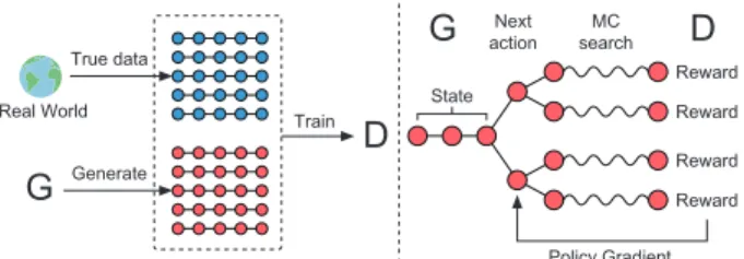
As a new way of training generative models, Generative Ad-versarial Net (GAN) that uses a discriminative model to guide the training of the generative model has enjoyed considerable success in generating real-valued data. However, it has limi-tations when the goal is for generating sequences of discrete tokens. A major reason lies in that the discrete outputs from the generative model make it difficult to pass the gradient up-date from the discriminative model to the generative model. Also, the discriminative model can only assess a complete sequence, while for a partially generated sequence, it is non-trivial to balance its current score and the future one once the entire sequence has been generated. In this paper, we pro-pose a sequence generation framework, called SeqGAN, to solve the problems. Modeling the data generator as a stochas-tic policy in reinforcement learning (RL), SeqGAN bypasses the generator differentiation problem by directly performing gradient policy update. The RL reward signal comes from the GAN discriminator judged on a complete sequence, and is passed back to the intermediate state-action steps using Monte Carlo search. Extensive experiments on synthetic data and real-world tasks demonstrate significant improvements over strong baselines.

Introduction

Generating sequential synthetic data that mimics the real one is an important problem in unsupervised learning. Re-cently, recurrent neural networks (RNNs) with long short-term memory (LSTM) cells (Hochreiter and Schmidhuber 1997) have shown excellent performance ranging from nat-ural language generation to handwriting generation (Wen et al. 2015; Graves 2013). The most common approach to training an RNN is to maximize the log predictive likelihood of each true token in the training sequence given the pre-vious observed tokens (Salakhutdinov 2009). However, as argued in (Bengio et al. 2015), the maximum likelihood ap-proaches suffer from so-calledexposure biasin the inference stage: the model generates a sequence iteratively and pre-dicts next token conditioned on its previously predicted ones that may be never observed in the training data. Such a dis-crepancy between training and inference can incur accumu-latively along with the sequence and will become prominent as the length of sequence increases. To address this prob-lem, (Bengio et al. 2015) proposed a training strategy called

∗

Weinan Zhang is the corresponding author.

Copyright c2017, Association for the Advancement of Artificial Intelligence (www.aaai.org). All rights reserved.

scheduled sampling (SS), where the generative model is par-tially fed with its own synthetic data as prefix (observed to-kens) rather than the true data when deciding the next token in the training stage. Nevertheless, (Husz´ar 2015) showed that SS is an inconsistent training strategy and fails to ad-dress the problem fundamentally. Another possible solution of the training/inference discrepancy problem is to build the loss function on the entire generated sequence instead of each transition. For instance, in the application of ma-chine translation, a task specific sequence score/loss, bilin-gual evaluation understudy (BLEU) (Papineni et al. 2002), can be adopted to guide the sequence generation. However, in many other practical applications, such as poem genera-tion (Zhang and Lapata 2014) and chatbot (Hingston 2009), a task specific loss may not be directly available to score a generated sequence accurately.

General adversarial net (GAN) proposed by (Goodfellow and others 2014) is a promising framework for alleviating the above problem. Specifically, in GAN a discriminative netDlearns to distinguish whether a given data instance is real or not, and a generative netGlearns to confuseD by generating high quality data. This approach has been suc-cessful and been mostly applied in computer vision tasks of generating samples of natural images (Denton et al. 2015).

Unfortunately, applying GAN to generating sequences has two problems. Firstly, GAN is designed for generat-ing real-valued, continuous data but has difficulties in di-rectly generating sequences of discrete tokens, such as texts (Husz´ar 2015). The reason is that in GANs, the genera-tor starts with random sampling first and then a determistic transform, govermented by the model parameters. As such, the gradient of the loss from D w.r.t. the outputs by Gis used to guide the generative modelG(paramters) to slightly change the generated value to make it more realistic. If the generated data is based on discrete tokens, the “slight change” guidance from the discriminative net makes little sense because there is probably no corresponding token for such slight change in the limited dictionary space (Goodfel-low 2016). Secondly, GAN can only give the score/loss for an entire sequence when it has been generated; for a partially generated sequence, it is non-trivial to balance how good as it is now and the future score as the entire sequence.

In this paper, to address the above two issues, we follow (Bachman and Precup 2015; Bahdanau et al. 2016) and con-sider the sequence generation procedure as a sequential de-cision making process. The generative model is treated as an

agent of reinforcement learning (RL); the state is the ated tokens so far and the action is the next token to be gener-ated. Unlike the work in (Bahdanau et al. 2016) that requires a task-specific sequence score, such as BLEU in machine translation, to give the reward, we employ a discriminator to evaluate the sequence and feedback the evaluation to guide the learning of the generative model. To solve the problem that the gradient cannot pass back to the generative model when the output is discrete, we regard the generative model as a stochastic parametrized policy. In our policy gradient, we employ Monte Carlo (MC) search to approximate the state-action value. We directly train the policy (generative model) via policy gradient (Sutton et al. 1999), which natu-rally avoids the differentiation difficulty for discrete data in a conventional GAN.

Extensive experiments based on synthetic and real data are conducted to investigate the efficacy and properties of the proposed SeqGAN. In our synthetic data environment, SeqGAN significantly outperforms the maximum likelihood methods, scheduled sampling and PG-BLEU. In three real-world tasks, i.e. poem generation, speech language gener-ation and music genergener-ation, SeqGAN significantly outper-forms the compared baselines in various metrics including human expert judgement.

Related Work

Deep generative models have recently drawn significant attention, and the ability of learning over large (unla-beled) data endows them with more potential and vitality (Salakhutdinov 2009; Bengio et al. 2013). (Hinton, Osin-dero, and Teh 2006) first proposed to use the contrastive di-vergence algorithm to efficiently training deep belief nets (DBN). (Bengio et al. 2013) proposed denoising autoen-coder (DAE) that learns the data distribution in a supervised learning fashion. Both DBN and DAE learn a low dimen-sional representation (encoding) for each data instance and generate it from a decoding network. Recently, variational autoencoder (VAE) that combines deep learning with sta-tistical inference intended to represent a data instance in a latent hidden space (Kingma and Welling 2014), while still utilizing (deep) neural networks for non-linear mapping. The inference is done via variational methods. All these gen-erative models are trained by maximizing (the lower bound of) training data likelihood, which, as mentioned by (Good-fellow and others 2014), suffers from the difficulty of ap-proximating intractable probabilistic computations.

(Goodfellow and others 2014) proposed an alternative training methodology to generative models, i.e. GANs, where the training procedure is a minimax game between a generative model and a discriminative model. This frame-work bypasses the difficulty of maximum likelihood learn-ing and has gained striklearn-ing successes in natural image gen-eration (Denton et al. 2015). However, little progress has been made in applying GANs to sequence discrete data gen-eration problems, e.g. natural language gengen-eration (Husz´ar 2015). This is due to the generator network in GAN is de-signed to be able to adjust the output continuously, which does not work on discrete data generation (Goodfellow 2016).

On the other hand, a lot of efforts have been made to gen-erate structured sequences. Recurrent neural networks can

be trained to produce sequences of tokens in many applica-tions such as machine translation (Sutskever, Vinyals, and Le 2014; Bahdanau, Cho, and Bengio 2014). The most pop-ular way of training RNNs is to maximize the likelihood of each token in the training data whereas (Bengio et al. 2015) pointed out that the discrepancy between training and gen-erating makes the maximum likelihood estimation subopti-mal and proposed scheduled sampling strategy (SS). Later (Husz´ar 2015) theorized that the objective function under-neath SS is improper and explained the reason why GANs tend to generate natural-looking samples in theory. Conse-quently, the GANs have great potential but are not practi-cally feasible to discrete probabilistic models currently.

As pointed out by (Bachman and Precup 2015), the se-quence data generation can be formulated as a sequen-tial decision making process, which can be potensequen-tially be solved by reinforcement learning techniques. Modeling the sequence generator as a policy of picking the next token, policy gradient methods (Sutton et al. 1999) can be adopted to optimize the generator once there is an (implicit) re-ward function to guide the policy. For most practical se-quence generation tasks, e.g. machine translation (Sutskever, Vinyals, and Le 2014), the reward signal is meaningful only for the entire sequence, for instance in the game of Go (Sil-ver et al. 2016), the reward signal is only set at the end of the game. In those cases, state-action evaluation methods such as Monte Carlo (tree) search have been adopted (Browne et al. 2012). By contract, our proposed SeqGAN extends GANs with the RL-based generator to solve the sequence generation problem, where a reward signal is provided by the discriminator at the end of each episode via Monte Carlo approach, and the generator picks the action and learns the policy using estimated overall rewards.

Sequence Generative Adversarial Nets

The sequence generation problem is denoted as follows. Given a dataset of real-world structured sequences, train a θ-parameterized generative model Gθ to produce a se-quence Y1:T = (y1, . . . , yt, . . . , yT), yt ∈ Y, whereY is

the vocabulary of candidate tokens. We interpret this prob-lem based on reinforcement learning. In timestept, the state

sis the current produced tokens(y1, . . . , yt−1)and the

ac-tionais the next tokenytto select. Thus the policy model Gθ(yt|Y1:t−1)is stochastic, whereas the state transition is

deterministic after an action has been chosen, i.e.δa_s,s0 = 1 for the next states0 _{= Y}

1:tif the current states =Y1:t−1

and the actiona=yt; for other next statess00,δas,s00= 0. Additionally, we also train aφ-parameterized discrimina-tive model Dφ (Goodfellow and others 2014) to provide a

guidance for improving generatorGθ.Dφ(Y1:T)is a

prob-ability indicating how likely a sequenceY1:T is from real

sequence data or not. As illustrated in Figure 1, the dis-criminative model Dφ is trained by providing positive ex-amples from the real sequence data and negative exex-amples from the synthetic sequences generated from the generative modelGθ. At the same time, the generative modelGθis up-dated by employing a policy gradient and MC search on the basis of the expected end reward received from the discrim-inative modelDφ. The reward is estimated by the likelihood

that it would fool the discriminative modelDφ. The specific formulation is given in the next subsection.

Reward Next action State MC search

G

D

Generate True data Train

G

Real World

D

Reward_Reward Reward Policy Gradient

Figure 1: The illustration of SeqGAN. Left:Dis trained over the real data and the generated data byG. Right:Gis trained by policy gradient where the final reward signal is provided byDand is passed back to the intermediate action value via Monte Carlo search.

SeqGAN via Policy Gradient

Following (Sutton et al. 1999), when there is no interme-diate reward, the objective of the generator model (policy)

Gθ(yt|Y1:t−1)is to generate a sequence from the start state s0to maximize its expected end reward:

J(θ) =E[RT|s0, θ] = X y1∈Y Gθ(y1|s0)·Q G_θ Dφ(s0, y1), (1) whereRT is the reward for a complete sequence. Note that the reward is from the discriminatorDφ, which we will dis-cuss later. QGθ

Dφ(s, a) is the action-value function of a se-quence, i.e. the expected accumulative reward starting from states, taking actiona, and then following policy Gθ. The rational of the objective function for a sequence is that start-ing from a given initial state, the goal of the generator is to generate a sequence which would make the discriminator consider it is real.

The next question is how to estimate the action-value function. In this paper, we use the REINFORCE algorithm (Williams 1992) and consider the estimated probability of being real by the discriminatorDφ(Y_1:n_T)as the reward. For-mally, we have:

QGθ

Dφ(a=yT, s=Y1:T−1) =Dφ(Y1:T). (2) However, the discriminator only provides a reward value for a finished sequence. Since we actually care about the long-term reward, at every timestep, we should not only consider the fitness of previous tokens (prefix) but also the resulted future outcome. This is similar to playing the games such as Go or Chess where players sometimes would give up the immediate interests for the long-term victory (Silver et al. 2016). Thus, to evaluate the action-value for an intermediate state, we apply Monte Carlo search with a roll-out policyGβ

to sample the unknown lastT −t tokens. We represent an

N-time Monte Carlo search as n Y1:1T, . . . , Y N 1:T o =MCGβ_(Y 1:t;N), (3)

whereY1:nt= (y1, . . . , yt)andYtn+1:T is sampled based on

the roll-out policyGβ and the current state. In our experi-ment,Gβ is set the same as the generator, but one can use a simplified version if the speed is the priority (Silver et al. 2016). To reduce the variance and get more accurate assess-ment of the action value, we run the roll-out policy starting from current state till the end of the sequence forNtimes to get a batch of output samples. Thus, we have:

QGθ Dφ(s=Y1:t−1, a=yt) = (4) ₁ N PN n=1Dφ(Y n 1:T), Y1:nT ∈MCGβ(Y1:t;N) for t < T Dφ(Y1:t) for t=T ,

where, we see that when no intermediate reward, the func-tion is iteratively defined as the next-state value starting from states0 =Y1:tand rolling out to the end.

A benefit of using the discriminatorDφas a reward

func-tion is that it can be dynamically updated to further improve the generative model iteratively. Once we have a set of more realistic generated sequences, we shall re-train the discrimi-nator model as follows:

min

φ −EY∼pdata[logDφ(Y)]−EY∼Gθ[log(1−Dφ(Y))]. (5)

Each time when a new discriminator model has been ob-tained, we are ready to update the generator. The proposed policy based method relies upon optimizing a parametrized policy to directly maximize the long-term reward. Following (Sutton et al. 1999), the gradient of the objective function

J(θ)w.r.t. the generator’s parametersθcan be derived as ∇θJ(θ) =EY1:t−1∼Gθ P yt∈Y ∇θGθ(yt|Y1:t−1)·QGDθφ(Y1:t−1, yt) . (6) The above form is due to the deterministic state transi-tion and zero intermediate rewards. The detailed derivatransi-tion is provided in the appendix. Using likelihood ratios (Glynn 1990; Sutton et al. 1999), we build an unbiased estimation for Eq. (6) (on one episode):

∇θJ(θ)' 1 T T X t=1 X yt∈Y ∇θGθ(yt|Y1:t−1)·Q Gθ Dφ(Y1:t−1, yt) (7) = 1 T T X t=1 X yt∈Y Gθ(yt|Y1:t−1)∇θlogGθ(yt|Y1:t−1)·QDGφθ(Y1:t−1, yt) = 1 T T X t=1 Eyt∼Gθ(yt|Y1:t−1)[∇θlogGθ(yt|Y1:t−1)·QDGθφ(Y1:t−1, yt)], whereY1:t−1 is the observed intermediate state sampled

fromGθ. Since the expectationE[·]can be approximated by

sampling methods, we then update the generator’s parame-ters as:

θ←θ+αh∇θJ(θ), (8) whereαh ∈ R+ denotes the corresponding learning rate

ath-th step. Also the advanced gradient algorithms such as Adam and RMSprop can be adopted here.

In summary, Algorithm 1 shows full details of the pro-posed SeqGAN. At the beginning of the training, we use the maximum likelihood estimation (MLE) to pre-trainGθ on

training setS. We found the supervised signal from the pre-trained discriminator is informative to help adjust the gener-ator efficiently.

After the pre-training, the generator and discriminator are trained alternatively. As the generator gets progressed via training on g-steps updates, the discriminator needs to be re-trained periodically to keeps a good pace with the generator. When training the discriminator, positive examples are from the given dataset S, whereas negative examples are gener-ated from our generator. In order to keep the balance, the number of negative examples we generate for each d-step is the same as the positive examples. And to reduce the vari-ability of the estimation, we use different sets of negative samples combined with positive ones, which is similar to bootstrapping (Quinlan 1996).

Algorithm 1Sequence Generative Adversarial Nets Require: generator policyGθ; roll-out policyGβ; discriminator

Dφ; a sequence datasetS={X1:T}

1: InitializeGθ,Dφwith random weightsθ, φ.

2: Pre-trainGθusing MLE onS

3: β←θ

4: Generate negative samples usingGθfor trainingDφ

5: Pre-trainDφvia minimizing the cross entropy

6: repeat 7: forg-stepsdo 8: Generate a sequenceY1:T= (y1, . . . , yT)∼Gθ 9: fortin1 :Tdo 10: ComputeQ(a=yt;s=Y1:t−1)by Eq. (4) 11: end for

12: Update generator parameters via policy gradient Eq. (8) 13: end for

14: ford-stepsdo

15: Use currentGθto generate negative examples and

com-bine with given positive examplesS

16: Train discriminatorDφforkepochs by Eq. (5)

17: end for 18: β←θ

19: untilSeqGAN converges

The Generative Model for Sequences

We use recurrent neural networks (RNNs) (Hochreiter and Schmidhuber 1997) as the generative model. An RNN maps the input embedding representations x1, . . . ,xT of

the sequence x1, . . . , xT into a sequence of hidden states

h1, . . . ,hT by using the update functiongrecursively.

ht=g(ht−1,xt) (9)

Moreover, a softmax output layerzmaps the hidden states into the output token distribution

p(yt|x1, . . . , xt) =z(ht) =softmax(c+V ht), (10)

where the parameters are a bias vectorcand a weight ma-trixV. To deal with the common vanishing and exploding gradient problem (Goodfellow, Bengio, and Courville 2016) of the backpropagation through time, we leverage the Long Short-Term Memory (LSTM) cells (Hochreiter and Schmid-huber 1997) to implement the update functiongin Eq. (9). It is worth noticing that most of the RNN variants, such as the gated recurrent unit (GRU) (Cho et al. 2014) and soft at-tention mechanism (Bahdanau, Cho, and Bengio 2014), can be used as a generator in SeqGAN.

The Discriminative Model for Sequences

Deep discriminative models such as deep neural network (DNN) (Vesel`y et al. 2013), convolutional neural network (CNN) (Kim 2014) and recurrent convolutional neural net-work (RCNN) (Lai et al. 2015) have shown a high perfor-mance in complicated sequence classification tasks. In this paper, we choose the CNN as our discriminator as CNN has recently been shown of great effectiveness in text (token se-quence) classification (Zhang and LeCun 2015). Most dis-criminative models can only perform classification well for an entire sequence rather than the unfinished one. In this pa-per, we also focus on the situation where the discriminator predicts the probability that a finished sequence is real.1

1_{In our work, the generated sequence has a fixed lengthT, but}

note that CNN is also capable of the variable-length sequence dis-crimination with the max-over-time pooling technique (Kim 2014).

We first represent an input sequencex1, . . . , xT as:

E1:T=x1⊕x2⊕. . .⊕xT, (11)

where xt ∈ Rk is the k-dimensional token embedding

and ⊕ is the concatenation operator to build the matrix

E1:T ∈ RT×k. Then a kernelw ∈ Rl×k applies a

convo-lutional operation to a window size oflwords to produce a new feature map:

ci=ρ(w⊗ Ei:i+l−1+b), (12) where ⊗operator is the summation of elementwise pro-duction, b is a bias term and ρ is a non-linear function. We can use various numbers of kernels with different win-dow sizes to extract different features. Finally we apply a max-over-time pooling operation over the feature maps

˜

c= max{c1, . . . , cT−l+1}.

To enhance the performance, we also add the highway ar-chitecture (Srivastava, Greff, and Schmidhuber 2015) based on the pooled feature maps. Finally, a fully connected layer with sigmoid activation is used to output the probability that the input sequence is real. The optimization target is to min-imize the cross entropy between the ground truth label and the predicted probability as formulated in Eq. (5).

Detailed implementations of the generative and discrimi-native models are provided in the appendix.

Synthetic Data Experiments

To test the efficacy and add our understanding of SeqGAN, we conduct a simulated test with synthetic data2_{. To simulate} the real-world structured sequences, we consider a language model to capture the dependency of the tokens. We use a randomly initialized LSTM as the true model, aka, the ora-cle, to generate the real data distributionp(xt|x1, . . . , xt−1)

for the following experiments.

Evaluation Metric

The benefit of having such oracle is that firstly, it provides the training dataset and secondly evaluates the exact perfor-mance of the generative models, which will not be possi-ble with real data. We know that MLE is trying to mini-mize the cross-entropy between the true data distributionp

and our approximationq, i.e.−Ex∼plogq(x). However, the

most accurate way of evaluating generative models is that we draw some samples from it and let human observers re-view them based on their prior knowledge. We assume that the human observer has learned an accurate model of the natural distributionphuman(x). Then in order to increase the chance of passing Turing Test, we actually need to min-imize the exact opposite average negative log-likelihood

−Ex∼qlogphuman(x)(Husz´ar 2015), with the role ofpand

qexchanged. In our synthetic data experiments, we can con-sider the oracle to be the human observer for real-world problems, thus a perfect evaluation metric should be

NLLoracle=−EY1:T∼Gθ h_XT t=1 logGoracle(yt|Y1:t−1) i , (13) whereGθ andGoracledenote our generative model and the oracle respectively.

At the test stage, we use Gθ to generate 100,000

se-quence samples and calculate NLLoraclefor each sample by

2

Table 1: Sequence generation performance comparison. The

p-value is between SeqGAN and the baseline from T-test. Algorithm Random MLE SS PG-BLEU SeqGAN

NLL 10.310 9.038 8.985 8.946 8.736 p-value <10−6 <10−6 <10−6 <10−6 0 50 100 150 200 250 Epochs 8.6 8.8 9.0 9.2 9.4 9.6 9.8 10.0 NLL by oracle Learning curve SeqGAN MLE Schedule Sampling PG­BLEU

Figure 2: Negative log-likelihood convergence w.r.t. the training epochs. The vertical dashed line represents the end of pre-training for SeqGAN, SS and PG-BLEU.

Goracle and their average score. Also significance tests are performed to compare the statistical properties of the gener-ation performance between the baselines and SeqGAN.

Training Setting

To set up the synthetic data experiments, we first initialize the parameters of an LSTM network following the normal distributionN(0,1) as the oracle describing the real data distributionGoracle(xt|x1, . . . , xt−1). Then we use it to

gen-erate 10,000 sequences of length 20 as the training setSfor the generative models.

In SeqGAN algorithm, the training set for the discrimina-tor is comprised by the generated examples with the label 0 and the instances fromS with the label 1. For different tasks, one should design specific structure for the convolu-tional layer and in our synthetic data experiments, the kernel size is from 1 toT and the number of each kernel size is be-tween 100 to 2003_{. Dropout (Srivastava et al. 2014) and L2} regularization are used to avoid over-fitting.

Four generative models are compared with SeqGAN. The first model is a random token generation. The second one is the MLE trained LSTMGθ. The third one is scheduled sam-pling (Bengio et al. 2015). The fourth one is the Policy Gra-dient with BLEU (PG-BLEU). In the scheduled sampling, the training process gradually changes from a fully guided scheme feeding the true previous tokens into LSTM, towards a less guided scheme which mostly feeds the LSTM with its generated tokens. A curriculum rateωis used to control the probability of replacing the true tokens with the generated ones. To get a good and stable performance, we decreaseω

by 0.002 for every training epoch. In the PG-BLEU algo-rithm, we use BLEU, a metric measuring the similarity be-tween a generated sequence and references (training data), to score the finished samples from Monte Carlo search.

Results

The NLLoracleperformance of generating sequences from the compared policies is provided in Table 1. Since the

evalua-3

Implementation details are in the appendix.

0 50 100 150 200 Epochs 8.70 8.94 9.00 9.50 10.00 NLL by oracle SeqGAN

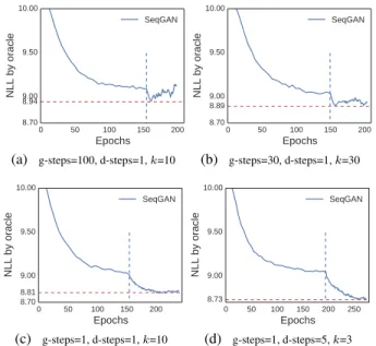
(a) g-steps=100, d-steps=1,k=10

0 50 100 150 200 Epochs 8.70 8.89 9.00 9.50 10.00 NLL by oracle SeqGAN (b) g-steps=30, d-steps=1,k=30 0 50 100 150 200 Epochs 8.70 8.81 9.00 9.50 10.00 NLL by oracle SeqGAN (c) g-steps=1, d-steps=1,k=10 0 50 100 150 200 250 Epochs 8.73 9.00 9.50 10.00 NLL by oracle SeqGAN (d) g-steps=1, d-steps=5,k=3 Figure 3: Negative log-likelihood convergence performance of SeqGAN with different training strategies. The vertical dashed line represents the beginning of adversarial training. tion metric is fundamentally instructive, we can see the im-pact of SeqGAN, which outperforms other baselines signif-icantly. A significance T-test on the NLLoraclescore distribu-tion of the generated sequences from the compared models is also performed, which demonstrates the significant im-provement of SeqGAN over all compared models.

The learning curves shown in Figure 4 illustrate the su-periority of SeqGAN explicitly. After about 150 training epochs, both the maximum likelihood estimation and the schedule sampling methods converge to a relatively high NLLoraclescore, whereas SeqGAN can improve the limit of the generator with the same structure as the baselines sig-nificantly. This indicates the prospect of applying adversar-ial training strategies to discrete sequence generative mod-els to breakthrough the limitations of MLE. Additionally, SeqGAN outperforms PG-BLEU, which means the discrim-inative signal in GAN is more general and effective than a predefined score (e.g. BLEU) to guide the generative policy to capture the underlying distribution of the sequence data.

Discussion

In our synthetic data experiments, we find that the stability of SeqGAN depends on the training strategy. More specifi-cally, the g-steps, d-steps andkparameters in Algorithm 1 have a large effect on the convergence and performance of SeqGAN. Figure 3 shows the effect of these parameters. In Figure 3(a), the g-steps is much larger than the d-steps and epoch number k, which means we train the generator for many times until we update the discriminator. This strategy leads to a fast convergence but as the generator improves quickly, the discriminator cannot get fully trained and thus will provide a misleading signal gradually. In Figure 3(b), with more discriminator training epochs, the unstable train-ing process is alleviated. In Figure 3(c), we train the genera-tor for only one epoch and then before the discriminagenera-tor gets fooled, we update it immediately based on the more realistic negative examples. In such a case, SeqGAN learns stably.

The d-steps in all three training strategies described above is set to 1, which means we only generate one set of nega-tive examples with the same number as the given dataset, and then train the discriminator on it for variouskepochs. But actually we can utilize the potentially unlimited num-ber of negative examples to improve the discriminator. This trick can be considered as a type of bootstrapping, where we combine the fixed positive examples with different neg-ative examples to obtain multiple training sets. Figure 3(d) shows this technique can improve the overall performance with good stability, since the discriminator is shown more negative examples and each time the positive examples are emphasized, which will lead to a more comprehensive guid-ance for training generator. This is in line with the theo-rem in (Goodfellow and others 2014). When analyzing the convergence of generative adversarial nets, an important as-sumption is that the discriminator is allowed to reach its op-timum givenG. Only if the discriminator is capable of dif-ferentiating real data from unnatural data consistently, the supervised signal from it can be meaningful and the whole adversarial training process can be stable and effective.

Real-world Scenarios

To complement the previous experiments, we also test Se-qGAN on several real-world tasks, i.e. poem composition, speech language generation and music generation.

Text Generation

For text generation scenarios, we apply the proposed Seq-GAN to generate Chinese poems and Barack Obama polit-ical speeches. In the poem composition task, we use a cor-pus4_{of 16,394 Chinese quatrains, each containing four lines} of twenty characters in total. To focus on a fully automatic solution and stay general, we did not use any prior knowl-edge of special structure rules in Chinese poems such as specific phonological rules. In the Obama political speech generation task, we use a corpus5_{, which is a collection of} 11,092 paragraphs from Obama’s political speeches.

We use BLEU score as an evaluation metric to measure the similarity degree between the generated texts and the human-created texts. BLEU is originally designed to auto-matically judge the machine translation quality (Papineni et al. 2002). The key point is to compare the similarity between the results created by machine and the references provided by human. Specifically, for poem evaluation, we set n-gram to be 2 (BLEU-2) since most words (dependency) in classi-cal Chinese poems consist of one or two characters (Yi, Li, and Sun 2016) and for the similar reason, we use BLEU-3 and BLEU-4 to evaluate Obama speech generation perfor-mance. In our work, we use the whole test set as the refer-ences instead of trying to find some referrefer-ences for the fol-lowing line given the previous line (He, Zhou, and Jiang 2012). The reason is in generation tasks we only provide some positive examples and then let the model catch the pat-terns of them and generate new ones. In addition to BLEU, we also choose poem generation as a case for human judge-ment since a poem is a creative text construction and human evaluation is ideal. Specifically, we mix the 20 real poems

4

http://homepages.inf.ed.ac.uk/mlap/Data/EMNLP14/

5

https://github.com/samim23/obama-rnn

Table 2: Chinese poem generation performance comparison. Algorithm Human score p-value BLEU-2 p-value

MLE 0.4165

0.0034 0.6670 <10−6

SeqGAN 0.5356 0.7389

Real data 0.6011 0.746

Table 3: Obama political speech generation performance. Algorithm BLEU-3 p-value BLEU-4 p-value

MLE 0.519

<10−6 0.416 _0.00014

SeqGAN 0.556 0.427

Table 4: Music generation performance comparison. Algorithm BLEU-4 p-value MSE p-value

MLE 0.9210

<10−6 22.38 0.00034

SeqGAN 0.9406 20.62

and 20 each generated from SeqGAN and MLE. Then 70 experts on Chinese poems are invited to judge whether each of the 60 poem is created by human or machines. Once re-garded to be real, it gets +1 score, otherwise 0. Finally, the average score for each algorithm is calculated.

The experiment results are shown in Tables 2 and 3, from which we can see the significant advantage of SeqGAN over the MLE in text generation. Particularly, for poem composi-tion, SeqGAN performs comparably to real human data.

Music Generation

For music composition, we use Nottingham6dataset as our training data, which is a collection of 695 music of folk tunes in midi file format. We study the solo track of each music. In our work, we use 88 numbers to represent 88 pitches, which correspond to the 88 keys on the piano. With the pitch sam-pling for every 0.4s7_{, we transform the midi files into} se-quences of numbers from 1 to 88 with the length 32.

To model the fitness of the discrete piano key patterns, BLEU is used as the evaluation metric. To model the fitness of the continuous pitch data patterns, the mean squared error (MSE) (Manaris et al. 2007) is used for evaluation.

From Table 4, we see that SeqGAN outperforms the MLE significantly in both metrics in the music generation task.

Conclusion

In this paper, we proposed a sequence generation method, SeqGAN, to effectively train generative adversarial nets for structured sequences generation via policy gradient. To our best knowledge, this is the first work extending GANs to generate sequences of discrete tokens. In our synthetic data experiments, we used an oracle evaluation mechanism to explicitly illustrate the superiority of SeqGAN over strong baselines. For three real-world scenarios, i.e., poems, speech language and music generation, SeqGAN showed excellent performance on generating the creative sequences. We also performed a set of experiments to investigate the robustness and stability of training SeqGAN. For future work, we plan to build Monte Carlo tree search and value network (Silver et al. 2016) to improve action decision making for large scale data and in the case of longer-term planning.

6

http://www.iro.umontreal.ca/˜lisa/deep/data

7

References

[Bachman and Precup 2015] Bachman, P., and Precup, D. 2015. Data generation as sequential decision making. In

NIPS, 3249–3257.

[Bahdanau et al. 2016] Bahdanau, D.; Brakel, P.; Xu, K.; et al. 2016. An actor-critic algorithm for sequence predic-tion.arXiv:1607.07086.

[Bahdanau, Cho, and Bengio 2014] Bahdanau, D.; Cho, K.; and Bengio, Y. 2014. Neural machine translation by jointly learning to align and translate. arXiv:1409.0473.

[Bengio et al. 2013] Bengio, Y.; Yao, L.; Alain, G.; and Vin-cent, P. 2013. Generalized denoising auto-encoders as gen-erative models. InNIPS, 899–907.

[Bengio et al. 2015] Bengio, S.; Vinyals, O.; Jaitly, N.; and Shazeer, N. 2015. Scheduled sampling for sequence predic-tion with recurrent neural networks. InNIPS, 1171–1179. [Browne et al. 2012] Browne, C. B.; Powley, E.;

White-house, D.; Lucas, S. M.; et al. 2012. A survey of monte carlo tree search methods.IEEE TCIAIG4(1):1–43. [Cho et al. 2014] Cho, K.; Van Merri¨enboer, B.; Gulcehre,

C.; et al. 2014. Learning phrase representations using RNN encoder-decoder for statistical machine translation.

EMNLP.

[Denton et al. 2015] Denton, E. L.; Chintala, S.; Fergus, R.; et al. 2015. Deep generative image models using a laplacian pyramid of adversarial networks. InNIPS, 1486–1494. [Glynn 1990] Glynn, P. W. 1990. Likelihood ratio gradient

estimation for stochastic systems. Communications of the ACM33(10):75–84.

[Goodfellow and others 2014] Goodfellow, I., et al. 2014. Generative adversarial nets. InNIPS, 2672–2680.

[Goodfellow, Bengio, and Courville 2016] Goodfellow, I.; Bengio, Y.; and Courville, A. 2016. Deep learning. 2015. [Goodfellow 2016] Goodfellow, I. 2016. Generative

adver-sarial networks for text.http://goo.gl/Wg9DR7. [Graves 2013] Graves, A. 2013. Generating sequences with

recurrent neural networks.arXiv:1308.0850.

[He, Zhou, and Jiang 2012] He, J.; Zhou, M.; and Jiang, L. 2012. Generating chinese classical poems with statistical machine translation models. InAAAI.

[Hingston 2009] Hingston, P. 2009. A turing test for com-puter game bots. IEEE TCIAIG1(3):169–186.

[Hinton, Osindero, and Teh 2006] Hinton, G. E.; Osindero, S.; and Teh, Y.-W. 2006. A fast learning algorithm for deep belief nets.Neural computation18(7):1527–1554.

[Hochreiter and Schmidhuber 1997] Hochreiter, S., and Schmidhuber, J. 1997. Long short-term memory. Neural computation9(8):1735–1780.

[Husz´ar 2015] Husz´ar, F. 2015. How (not) to train your gen-erative model: Scheduled sampling, likelihood, adversary?

arXiv:1511.05101.

[Kim 2014] Kim, Y. 2014. Convolutional neural networks for sentence classification. arXiv:1408.5882.

[Kingma and Welling 2014] Kingma, D. P., and Welling, M. 2014. Auto-encoding variational bayes. ICLR.

[Lai et al. 2015] Lai, S.; Xu, L.; Liu, K.; and Zhao, J. 2015. Recurrent convolutional neural networks for text classifica-tion. InAAAI, 2267–2273.

[Manaris et al. 2007] Manaris, B.; Roos, P.; Machado, P.; et al. 2007. A corpus-based hybrid approach to music anal-ysis and composition. InNCAI, volume 22, 839.

[Papineni et al. 2002] Papineni, K.; Roukos, S.; Ward, T.; and Zhu, W.-J. 2002. Bleu: a method for automatic eval-uation of machine translation. InACL, 311–318.

[Quinlan 1996] Quinlan, J. R. 1996. Bagging, boosting, and c4. 5. InAAAI/IAAI, Vol. 1, 725–730.

[Salakhutdinov 2009] Salakhutdinov, R. 2009. Learning deep generative models. Ph.D. Dissertation, University of Toronto.

[Silver et al. 2016] Silver, D.; Huang, A.; Maddison, C. J.; Guez, A.; Sifre, L.; et al. 2016. Mastering the game of go with deep neural networks and tree search. Nature

529(7587):484–489.

[Srivastava et al. 2014] Srivastava, N.; Hinton, G. E.; Krizhevsky, A.; Sutskever, I.; and Salakhutdinov, R. 2014. Dropout: a simple way to prevent neural networks from overfitting.JMLR15(1):1929–1958.

[Srivastava, Greff, and Schmidhuber 2015] Srivastava, R. K.; Greff, K.; and Schmidhuber, J. 2015. Highway networks. arXiv:1505.00387.

[Sutskever, Vinyals, and Le 2014] Sutskever, I.; Vinyals, O.; and Le, Q. V. 2014. Sequence to sequence learning with neural networks. InNIPS, 3104–3112.

[Sutton et al. 1999] Sutton, R. S.; McAllester, D. A.; Singh, S. P.; Mansour, Y.; et al. 1999. Policy gradient methods for reinforcement learning with function approximation. In

NIPS, 1057–1063.

[Vesel`y et al. 2013] Vesel`y, K.; Ghoshal, A.; Burget, L.; and Povey, D. 2013. Sequence-discriminative training of deep neural networks. InINTERSPEECH, 2345–2349.

[Wen et al. 2015] Wen, T.-H.; Gasic, M.; Mrksic, N.; Su, P.-H.; Vandyke, D.; and Young, S. 2015. Semantically condi-tioned LSTM-based natural language generation for spoken dialogue systems. arXiv:1508.01745.

[Williams 1992] Williams, R. J. 1992. Simple statistical gradient-following algorithms for connectionist reinforce-ment learning. Machine learning8(3-4):229–256.

[Yi, Li, and Sun 2016] Yi, X.; Li, R.; and Sun, M. 2016. Generating chinese classical poems with RNN encoder-decoder. arXiv:1604.01537.

[Zhang and Lapata 2014] Zhang, X., and Lapata, M. 2014. Chinese poetry generation with recurrent neural networks. InEMNLP, 670–680.

[Zhang and LeCun 2015] Zhang, X., and LeCun, Y. 2015. Text understanding from scratch. arXiv:1502.01710.

Appendix

In Section 1, we present the step-by-step derivation of Eq. (6) in the paper. In Section 2, the detailed realization of the generative model and the discriminative model is discussed, including the model parameter settings. In Section 3, an interesting ablation study is provided, which is a supplementary to the discussions of the synthetic data experiments.

Proof for Eq. (6)

For readability, we provide the detailed derivation of Eq. (6) here by following (Sutton et al. 1999).

As mentioned in SEQUENCEGENERATIVEADVERSARIALNETSsection, the state transition is deterministic after an action has been chosen, i.e.δa

s,s0 = 1for the next states0 =Y1:tif the current states=Y1:t−1and the actiona=yt; for other next

statess00,δa

s,s00= 0. In addition, the intermediate rewardRa_sis 0. We re-write the action value and state value as follows:

QGθ_(s=Y 1:t−1, a=yt) =Ras+ X s0_∈S δssa0VGθ(s0) =VGθ(Y1:t) (14) VGθ_(s=Y 1:t−1) = X yt∈Y Gθ(yt|Y1:t−1)·QGθ(Y1:t−1, yt) (15)

For the start states0, the value is calculated as VGθ_(s

0) =E[RT|s0, θ] (16)

= X

y1∈Y

Gθ(y1|s0)·QGθ(s0, y1),

which is the objective functionJ(θ)to maximize in Eq. (1) of the paper.

Then we can obtain the gradient of the objective function, defined in Eq. (1), w.r.t. the generator’s parametersθ:

∇θJ(θ) =∇θVGθ_{(s0) =∇θ[}X y1∈Y Gθ(y1|s0)·QGθ(s0, y1)] = X y1∈Y [∇θGθ(y1|s0)·QGθ(s0, y1) +Gθ(y1|s0)· ∇θQGθ(s0, y1)] = X y1∈Y [∇θGθ(y1|s0)·QGθ(s0, y1) +Gθ(y1|s0)· ∇θVGθ(Y1:1)] = X y1∈Y ∇θGθ(y1|s0)·QGθ(s0, y1) + X y1∈Y Gθ(y1|s0)∇θ[ X y2∈Y Gθ(y2|Y1:1)QGθ(Y1:1, y2)] = X y1∈Y ∇θGθ(y1|s0)·QGθ(s0, y1) + X y1∈Y Gθ(y1|s0) X y2∈Y [∇θGθ(y2|Y1:1)·QGθ(Y1:1, y2) +Gθ(y2|Y1:1)∇θQGθ(Y1:1, y2)] = X y1∈Y ∇θGθ(y1|s0)·QGθ(s0, y1) + X Y1:1 P(Y1:1|s0;Gθ) X y2∈Y ∇θGθ(y2|Y1:1)·QGθ(Y1:1, y2) +X Y1:2 P(Y1:2|s0;Gθ)∇θVGθ(Y1:2) = T X t=1 X Y1:t−1 P(Y1:t−1|s0;Gθ) X yt∈Y ∇θGθ(yt|Y1:t−1)·QGθ(Y1:t−1, yt) =EY1:t−1∼Gθ[ X yt∈Y ∇θGθ(yt|Y1:t−1)·QGθ(Y1:t−1, yt)], (17)

which is the result in Eq. (6) of the paper.

Model Implementations

The Generative Model for Sequences We use recurrent neural networks (RNNs) (Hochreiter and Schmidhuber 1997) as the generative model. An RNN maps the input embedding representationsx1, . . . ,xT of the sequencex1, . . . , xT into a sequence

of hidden statesh1, . . . ,hT by using the update functiongrecursively.

ht=g(ht−1,xt) (18)

Moreover, a softmax output layerzmaps the hidden states into the output token distribution

p(yt|x1, . . . , xt) =z(ht) =softmax(c+V ht), (19)

where the parameters are a bias vectorcand a weight matrixV.

The vanishing and exploding gradient problem in backpropagation through time (BPTT) issues a challenge of learning long-term dependencies to recurrent neural network (Goodfellow, Bengio, and Courville 2016). To address such problems, gated RNNs have been designed based on the basic idea of creating paths through time that have derivatives that neither vanish nor explode. Among various gated RNNs, we choose the Long Short-Term Memory (LSTM) (Hochreiter and Schmidhuber 1997) to be our generative networks with the update equations:

ft=σ(Wf·[ht−1,xt] +bf), it=σ(Wi·[ht−1,xt] +bi), ot=σ(Wo·[ht−1,xt] +bo), st=ftst−1+ittanh(Ws·[ht−1,xt] +bs), ht=ottanh(st), (20)

where[h,x]is the vector concatenation andis the elementwise product.

For simplicity, we use the standard LSTM as the generator, while it is worth noticing that most of the RNN variants, such as the gated recurrent unit (GRU) (Cho et al. 2014) and soft attention mechanism (Bahdanau, Cho, and Bengio 2014), can be used as a generator in SeqGAN.

The standard way of training an RNNGθis the maximum likelihood estimation (MLE), which involves minimizing the

neg-ative log-likelihood−PT

t=1logGθ(yt=xt| {x1, . . . , xt−1})for a generated sequence(y1, . . . , yT)given input(x1, . . . , xT).

However, when applying MLE to generative models, there is a discrepancy between training and generating (Bengio et al. 2015; Husz´ar 2015), which motivates our work.

The Discriminative Model for Sequences Deep discriminative models such as deep neural network (DNN) (Vesel`y et al. 2013), convolutional neural network (CNN) (Kim 2014) and recurrent convolutional neural network (RCNN) (Lai et al. 2015) have shown a high performance in complicated sequence classification tasks. In this paper, we choose the CNN as our dis-criminator as CNN has recently been shown of great effectiveness in text (token sequence) classification (Zhang and LeCun 2015).

As far as we know, except for some specific tasks, most discriminative models can only perform classification well for a whole sequence rather than the unfinished one. In case of some specific tasks, one may design a classifier to provide intermediate reward signal to enhance the performance of our framework. But to make it more general, we focus on the situation where discriminator can only provide final reward, i.e., the probability that a finished sequence was real.

We first represent an input sequencex1, . . . , xT as:

E1:T =x1⊕x2⊕. . .⊕xT, (21)

wherext∈Rkis thek-dimensional token embedding and⊕is the vertical concatenation operator to build the matrixE1:T ∈ RT×k. Then a kernelw∈Rl×k applies a convolutional operation to a window size oflwords to produce a new feature map:

ci=ρ(w⊗ Ei:i+l−1+b), (22)

where⊗operator is the summation of elementwise production,b is a bias term andρis a non-linear function. We can use various numbers of kernels with different window sizes to extract different features. Specifically, a kernelwwith window size

lapplied to the concatenated embeddings of input sequence will produce a feature map

c= [c1, . . . , cT−l+1]. (23)

Finally we apply a max-over-time pooling operation over the feature map˜c = max{c}and pass all pooled features from different kernels to a fully connected softmax layer to get the probability that a given sequence is real.

We perform an empirical experiment to choose the kernel window sizes and numbers as shown in Table 5. For different tasks, one should design specific structures for the discriminator.

To enhance the performance, we also add the highway architecture (Srivastava, Greff, and Schmidhuber 2015) before the final fully connected layer:

τ =σ(WT ·c˜+bT), ˜

C=τ·H(˜c,WH) + (1−τ)·c˜,

Table 5: Convolutional layer structures. Sequence length (window size, kernel numbers)

20 (1, 100),(2, 200),(3, 200),(4, 200),(5, 200) (6, 100),(7, 100),(8, 100),(9, 100),(10, 100) (15, 160),(20, 160) 32 (1, 100),(2, 200),(3, 200),(4, 200),(5, 200) (6, 100),(7, 100),(8, 100),(9, 100),(10, 100) (16, 160),(24, 160),(32, 160)

whereWT,bTandWHare highway layer weights,Hdenotes an affine transform followed by a non-linear activation function

such as a rectified linear unit (ReLU) andτis the “transform gate” with the same dimensionality asH(˜c,WH)andc˜. Finally,

we apply a sigmoid transformation to get the probability that a given sequence is real:

ˆ

y=σ(Wo·C˜ +bo) (25)

whereWoandbois the output layer weight and bias.

When optimizing discriminative models, supervised training is applied to minimize the cross entropy, which is widely used as the objective function for classification and prediction tasks:

L(y,yˆ) =−ylog ˆy−(1−y) log(1−yˆ), (26)

whereyis the ground truth label of the input sequence andyˆis the predicted probability from the discriminative models.

More Ablation Study

0 50 100 150 200 250 300 350 400

Epochs

8.6 8.8 9.0 9.2 9.4 9.6 9.8 10.0

NLL by oracle

SeqGAN with insufficient pre­training

SeqGAN with sufficient pre­training

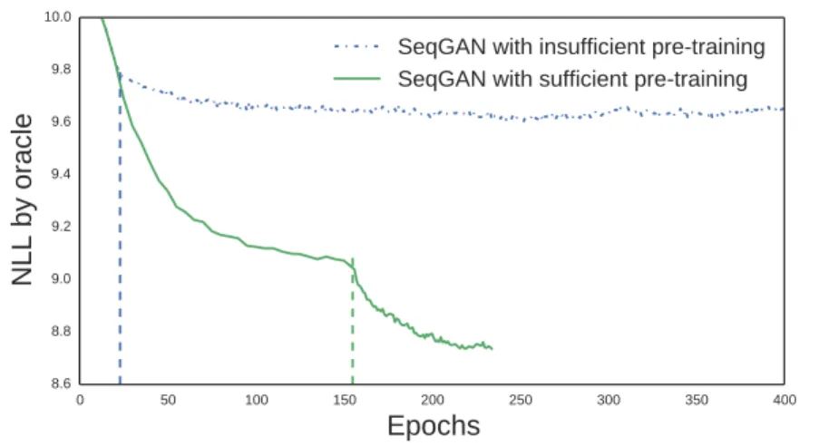
Figure 4: Negative log-likelihood performance with different pre-training epochs before the adversarial training. The vertical dashed lines represent the start of adversarial training.

In the DISCUSSIONsubsection of SYNTHETICDATAEXPERIMENTSsection of our paper, we discussed the ablation study of three hyperparameters of SeqGAN, i.e., g-steps, d-steps andkepoch number. Here we provide another ablation study which is instructive for the better training of SeqGAN.

As described in our paper, we start the adversarial training process after the convergence of MLE supervised pre-training. Here we further conduct experiments to investigate the performance of SeqGAN when the supervised pre-training is insufficient. As shown in Figure 4, if we pre-train the generative model with conventional MLE methods for only 20 epochs, which is far from convergence, then the adversarial training process improves the generator quite slowly and unstably. The reason is that in SeqGAN, the discriminative model provides reward guidance when training the generator and if the generator acts almost randomly, the discriminator will identify the generated sequence to be unreal with high confidence and almost every action the generator takes receives a low (unified) reward, which does not guide the generator towards a good improvement direction, resulting in an ineffective training procedure. This indicates that in order to apply adversarial training strategies to sequence generative models, a sufficient pre-training is necessary.