On Controlling the Size
of Clusters in Probabilistic Clustering
Aditya Jitta, Arto Klami
Helsinki Institute for Information Technology HIIT, Department of Computer Science, University of Helsinki
Abstract
Classical model-based partitional clustering algorithms, such as k-means or mixture of Gaussians, provide only loose and indirect control over the size of the resulting clusters. In this work, we present a family of probabilistic clustering models that can be steered towards clusters of desired size by pro-viding a prior distribution over the possible sizes, allowing the analyst to fine-tune exploratory analysis or to produce clusters of suitable size for future down-stream processing. Our formulation supports arbitrary multimodal prior distri-butions, generalizing the previous work on clustering algo-rithms searching for clusters of equal size or algoalgo-rithms de-signed for the microclustering task of finding small clusters. We provide practical methods for solving the problem, using integer programming for making the cluster assignments, and demonstrate that we can also automatically infer the number of clusters.
Introduction
Clustering is a canonical data analysis and machine learning tool for discovering group structure underlying the data. In this work, we study partitional clustering algorithms (meth-ods that partition the data space into disjoint regions) from the perspective of thecardinality of the clusters, presenting algorithms that allow the user to provide prior information on the desired number of objects in typical clusters.
Standard model-based partitional clustering algorithms, such as the classical k-means algorithm and probabilistic mixtures (McLachlan and Peel 2004) (e.g. Gaussian mixture model), are agnostic to the size of the clusters. The user can (and often has to) specify the desired number of clusters, but has very limited control over the size distribution of the clus-ters. Instead, it is determined implicitly via the model and the learning algorithm. For example, k-means prefers clus-ters of equal size whereas mixture models allow expressing preference on the relative sizes, but neither method enforces these preferences and the practical result may deviate sig-nificantly from the expected one. Non-parametric clustering models proposed for automatizing the choice of the num-ber of clusters, such as the Dirichlet process mixture (Teh 2010), do this at the cost of losing even more of the con-trol since the process underlying the choice of complexity Copyright c2018, Association for the Advancement of Artificial Intelligence (www.aaai.org). All rights reserved.
explicitly encodes preferences on the size distribution. See Miller and Harrison (2013) for good explanation of how Dirichlet process encourages the so-called rich-get-richer-property: it provides solutions consisting of a few large clus-ters and a large set of small clusclus-ters.
The lack of control for the size stems from a seemingly innocent modeling assumption behind partitional clustering algorithms: the objects are assumed independent and identi-cally distributed (i.i.d). Each object independently chooses its cluster allocation, which enables computationally effi-cient algorithms but prevents explicit control for cluster sizes. A natural remedy, suggested by Klami and Jitta (2016) in the context of microclustering, is to consider models with i.i.d. clusters instead: The data collection is generated as a set of K independent clusters that each independently choose how many objects to generate, instead of directly generatingN independent objects that map to theK clus-ters. Making this transition for, e.g. mixtures of Gaussians, is easy at the level of the model specification, but unfortu-nately results in computational challenges since the cluster allocations for theN samples now need to be carried out jointly by some form of constrained optimization. We will address these challenges in this work.
Various specific clustering models addressing the size dis-tribution have been proposed before. Bennett, Bradley, and Demiriz (2000) avoided empty clusters by setting a mini-mum size for each cluster, Banerjee and Ghosh (2006) stud-ied a variant of k-means that enforces equal size for all clus-ters, and Zhu, Wang, and Li (2010) consider algorithms that take arbitrary pre-determined cluster sizes as inputs for ex-ample to attempt solving classification problems with clus-tering algorithms. Perhaps the most closely related con-cept, however, is that ofmicroclustering(Miller et al. 2015; Klami and Jitta 2016) that searches for clustering solutions where the number of clusters K grows sub-linearly with the number of objects N; intuitively this corresponds to clustering solutions guaranteed to return small clusters. Our formulation generalizes theirs by allowing arbitrary priors on cluster sizes, and we provide considerably more effi-cient algorithms by focusing on maximum a posteriori so-lutions instead of attempting fully Bayesian analysis that re-quires either inefficient sample-by-sample allocation (Miller et al. 2015) or solving weighted discrete sampling problems (Klami and Jitta 2016) – while Bayesian inference is in
gen-The Thirty-Second AAAI Conference on Artificial Intelligence (AAAI-18)
eral desirable, for clustering applications we often want a point estimate for the cluster allocations in the end and hence it does not necessarily pay off to solve an unnecessarily com-plex problem.
Our quest for controlling the size of the clusters can be motivated from two perspectives: (i) Guiding clustering when used for exploratory analysis, and (ii) Enabling use of clustering for applications where the clusters are fed for future down-stream processing. In exploratory analysis the goal is to gain insight for an unknown data source, which is often very ill-defined problem, and hence all techniques that allow steering the process by additional prior knowl-edge are helpful. Existing techniques include for example methods that can take into account must-link and cannot-link constraints between objects (Wagstaff et al. 2001), pos-sibly run in an interactive manner to allow adapting the so-lution if unsatisfied with the results (Balcan and Blum 2008; Awasthi, Balcan, and Voevodski 2014). Our tools enable the analyst to provide prior information on size of the desired clusters. This can be helpful e.g. when using clustering to discover gene regulatory networks (D’haeseleer, Liang, and Somogyi 2000); multimodal prior over the number of genes typically involved in such networks helps discovering bio-logically plausible clusters. The second motivation is con-ceptually very different but can still be reached with the same techniques: If clustering is used not for exploration but as tool to distributing a set of objects into further processing e.g. by means of crowd-sourcing or to create teams of simi-lar individuals (Kim et al. 2015), we would like to be able to control the size of the clusters to get balanced solutions. Be-ing able to control for cluster sizes is also important when aligning clusters discovered in multiple data sources (Jitta and Klami 2017).
The core technical challenges in our work relate to the joint assignment of all objects into the clusters so that the cluster sizes adhere to the preferences. This needs to be car-ried out by constrained optimization, as observed already by Bennett, Bradley, and Demiriz (2000) and several others in restricted special cases. In this work we provide two practi-cal solutions for the problem, demonstrate them in the con-text of a simple mixture-based clustering model, and ana-lyze their properties empirically. We also highlight how the model family supports automatically selecting the number of clusters. The analyst needs to indicate the preferred cluster sizes by providing a suitable prior, but need not provide ad-ditional technical parameters such as the number of clusters that is often asked for as the first input in classical clustering algorithms.
Problem Formulation
The specific problem addresses in this paper is to cluster
Nobjectsxnrepresented byD-dimensional vectors intoK clusters such that the cluster sizessk (the number of sam-ples in each cluster) follow a prior probability distribution
p(s)specified by the analyst. In particular, we provide so-lutions that make no assumptions onp(s)other than it is a probability distribution over non-negative integers. We solve this problem using probabilistic partitional clustering algo-rithms, presenting an extension of mixture models to
sup-port such prior distributions, and search for parameters cor-responding to themaximum a posteriori(MAP) solution.
Related Work
In the following we discuss related work on a more technical level, highlighting how the proposed formulation advances the state-of-the-art.
Perhaps the most closely related work is on the concept ofmicroclusteringproposed recently by Miller et al. (2015) to denote clustering solutions where the size of the clusters grows sub-linearly with the number of objects in the data collection. They achieve this by imposing a negative bino-mial prior on the cluster size, and Klami and Jitta (2016) proposed an alternative microclustering model using hard constraints for the cluster size. Our solution generalizes on theirs by supporting arbitrary prior distributions on the clus-ter sizes, instead of limiting to the special case of unimodal priors that lead to small clusters. Furthermore, we provide considerably more scalable algorithms by focusing on MAP estimate instead of full Bayesian inference. Full Bayesian analysis is important when focusing on small clusters, but in general setups we typically want to report a point estimate, a single clustering solution, for the analyst anyway.
Some interactive clustering algorithms focus on the size of the clusters as well, by letting the analyst provide feed-back to achieve desired clustering results. Balcan and Blum (2008) presented techniques that allow splitting individ-ual clusters or merging two clusters, and Awasthi, Balcan, and Voevodski (2014) proposed localized algorithms for the same problem, letting the algorithm re-assign only objects in the indicated clusters. In this work we do not build an in-teractive clustering model as such, but instead consider prior preferences on cluster sizes as an alternative for an interac-tive procedure.
Our method is closely related to several clustering meth-ods that use constrained optimization for making the clus-ter assignments. Bennett, Bradley, and Demiriz (2000) used a minimum cost flow formulation to solve k-means prob-lems with minimum requirement for cluster sizes to prevent empty clusters, and Banerjee and Ghosh (2006) provided al-gorithms for k-means with roughly balanced cluster sizes. Zhu, Wang, and Li (2010) and Malinen and Fr¨anti (2014) extended this line of work to models where the desired size for each cluster can vary and is provided, for example, by ex-isting class labels, and Rujeerapaiboon et al. (2017) added support for outliers. Our formulation belongs to this fam-ily of methods, but supports more general prior information on the sizes, including complicated and potentially multi-modal prior distributions. Our algorithmic choices are also more general; we use simple integer program formulations and generic solvers to support arbitrary priors. The special cases described above can typically be solved more effi-ciently with algorithms tuned for each case.
Finally, it is worth mentioning that constrained optimiza-tion enables also directly solving clustering problems based on pairwise distances, for example using correlation clus-tering(Bansal, Blum, and Chawla 2004). We focus solely on partitional clustering models that explicitly represent the clusters.
Model and Methods
We consider clustering models from a probabilistic perspec-tive, working with generative models for a given finite data collection X = {xn}Nn=1 where the objects xn are typi-cally described by a set of some D features. The models are specified using N latent variables zn that indicate the cluster choice for each object, andKdistributions that gen-erate the observations conditional on the cluster allocation (parameterized byθk).
A prototypical example of this family is a finite mixture model (McLachlan and Peel 2004), for which the joint den-sity factorizes over the samples as
p(X, Z|θ) = N n=1 K k=1 [p(zn=k)p(xn|θk)]I[zn=k], whereI[·] is the identity function that evaluates to one if the input is true and to zero otherwise. With the choice of
p(xn|θk = {μk,Σk}) = N(μk,Σk)(normal distribution with mean μk and covarianceΣk) and p(zn) = Mult(π) (multinomial distribution withK-dimensional cluster prob-ability parameterπ) we get the mixture of Gaussians model. An important practical detail for such mixtures is that during inference, we can treat each sample independently when updating the cluster allocations since p(Z|X, θ) =
N
n=1p(zn|xn, θ), enabling efficient expectation maximiza-tion and Gibbs sampling algorithms.
The model we propose for mixture-based clustering with explicit control for cluster sizes replaces the i.i.d. samples with i.i.d. clusters. That is, the joint density is now factorized as p(X, Z|θ) = K k=1 p(sk) N n=1 p(xn|θk)I[zn=k] , (1) wheresk indicates the number of samples in thekth clus-ter. This formulation allows expressing prior preference on cluster sizes by specifying a suitable probability for p(s), but the convenience of updating the cluster allocations for each sample independently is lost: The conditional proba-bilityp(Z|X, θ)no longer factorizes over the samples.
Without a factorizing conditional the cluster assignment step becomes computationally more difficult, and can be solved by two alternative strategies. Miller et al. (2015) pro-posed algorithms that update the allocation for each of the object at a time based onp(zn|Z−n, X, θ), explicitly con-ditioning on allocations of all other samples (but marginal-izing over θ). Such a procedure, however, converges very slowly (or not at all) for various interesting choices ofp(s), such as multimodal distributions or distributions with very narrow support. The other solution, adopted in this work as well, is to jointly determine all of the allocations Z using constrained optimization. This strategy requires more com-putation for performing the allocations, but converges faster. For maximizing the joint density (1) we consider a generic alternating algorithm. Given an initial choice forθk, we al-ternate between
1. Estimate new allocation Z jointly for all samples based onp(Z|X, θ)
2. Estimate new parametersθkindependently for every clus-ter given p(θk|Xk), where Xk collects the samples for whichzn =k
In this work, we seek for the maximum a posterior solu-tion, which means the first step corresponds to a simple con-strained optimization problem. For full Bayesian analysis this step would need to be replaced by enumeration of all possible allocations with sufficiently large likelihood, which scales only for very small problems; Klami and Jitta (2016) adopted this choice and had to limit their experiments to problems with at most hundreds of objects.
Since the second step depends on the particular likelihood chosen as the data-generating distribution and is identical to standard mixture modeling, we will not describe the de-tails for that part. Instead, we will next explain two practical methods for solving the first step for various choices ofp(s).
Methods for Cluster Assignment
The assignment is found by maximizing the joint log-likelihood
logp(Z|X, θ) = logp(X|θ, Z) + logp(Z)
= n logp(xn|θzn) + k logp(sk), (2) which has to be solved for allznsimultaneously becausesk counts the number of objects assigned to thekth cluster.
The necessary inputs for any method solving this can be collected in a matrix
Cnk= logp(xn|θk)
storing the log-likelihoods of the individual data points for all cluster choices and a vector
da = logp(s=Sa)
storing the log-priors for possible cluster sizes. We denote byS ={S1, . . . SA}the support of the probabilityp(s), so thatS1indicates the smallest possible cluster size with non-zero probability andSAindicates the largest possible cluster size.Acounts the number of possible cluster sizes, but the values in setSneed not be contiguous.
In the following we present two practical methods that find the assignment maximizing the likelihood using con-strained optimization. The first poses the problem as binary integer program and the other as a mixed integer program, and we use standard solvers, here Gurobi, for solving them.
Method 1: Arbitrary Priors
The joint assignment problem can be solved for arbitrary prior distributions by formulating it as a binary integer prob-lem, parameterized by a matrix Π ∈ [0,1]N×K where
Πnk = 1 indicates the nth sample is assigned to the kth cluster, and by a matrixBka ∈ [0,1]K×A whereBka = 1 indicates thekth cluster has exactlySaobjects. Each row in
ΠandB is special ordered set of type 1 (SOS1), meaning that at exactly one element can be non-zero.
Given the above parameterization the joint assignment can be solved by the following binary integer problem:
max N n=1 K k=1 Cnk×Πnk+ K k=1 A a=1 Bk,a×da (3) s.t. K k=1 Πnk= 1 ∀n A a=1 Bk,a= 1 ∀k N n=1 Πnk=A a=1 Bk,a×Sa ∀k,
where the multiplication×is element-wise. The objective itself is simply the joint likelihood, the first two constraints encode the SOS1 property of the indicator matrices, and the third constraint guarantees the indicators Bka capture the cluster sizes. The method is applicable for all possible priors since the objective is encoded by binary variables selecting a suitable element fromd, and scales in complexity as a func-tion of the widthAof the support ofp(s). It has(N+A)K
binary variables andN+ 2Kconstraints, of whichN+K
correspond to SOS1.
An important property of the above formulation is that by settingS1 = 0we can provide non-zero probability for
empty clusters. By further lettingKto be sufficiently large number, the method can vary the number of clusters actu-ally being used for modeling the data and hence provides means for automatic complexity control. This is an alterna-tive to traditional non-parametric Bayesian models, such as Dirichlet process mixtures (Teh 2010), for controlling the complexity.
Method 2: Log-concave Priors
The method presented above works for arbitrary prior distri-butions, but it pays off to consider dedicated algorithms for restricted classes of priors on cluster sizes. One particularly interesting special case is unimodal prior distributions that indicate preference for a given size of clusters. Many natu-ral ways of encoding such preference can be provided with priors that are log-concave (e.g. normal distribution, uniform distribution over convex sets, Poisson, and the negative bino-mial distribution used by Miller et al. (2015) for microclus-tering), and it pays off to attempt constructing more efficient methods for this special case.
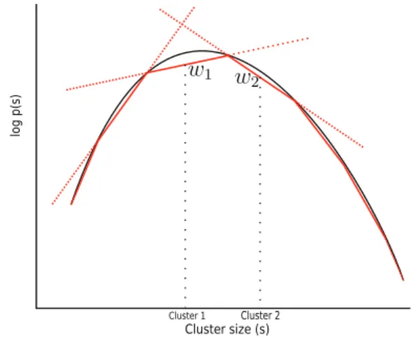
A natural way to solve constrained maximization prob-lems with concave losses is to provide a piece-wise linear approximation for the loss, and then replace the loss with a real-valued free parameter constrained to lie below the en-velope formed by the line segments. In optimal solution the free parameter always lies on one of the segments, corre-sponding to linear approximation of the original loss. We apply this technique for the second part of the objective in (2) as illustrated in Figure 1. The prior log-probability of ev-ery cluster is indicated bywk that is bounded from above byJ line segments, characterized by their interceptIj and
Cluster 1 Cluster 2
log p(s)
Cluster size (s)
Figure 1: Illustration of mixed integer program formulation for the cluster assignment. The log-prior for the cluster sizes (solid black line) is approximated with a piece-wise linear function (solid red lines), and for every cluster we assign a real-valued variable wk constrained to lie below the enve-lope formed by the linear segments. In optimal solutionwk always lies on the segment corresponding to the current clus-ter size; the dotted continuations of other line segments are used as constraints but are inactive in the optimal solution.
slopeΔj. The approximation for the prior is constructed be-fore running the method.
The full formulation of the assignment problem as mixed integer program is then
maxN n=1 K k=1 Cnk×Πnk+ K k=1 wk (4) s.t. K k=1 Πnk= 1 ∀n wk≤Ij+skΔj ∀k, j, (5) wheresk =nΠnkis the size of thekth cluster. This for-mulation hasN Kbinary variables andKreal variables with
NSOS1 constraints andKJinequality constraints. In prtice the number of line segments required for sufficiently ac-curate approximation for the prior depends on the widthA
of the support ofp(s). In our experiments we setJto 1/4 of
A, but note that the results would not change qualitatively unless using very smallJ.
Implementation Details
The practical performance of the generic method described above depends on a couple of small details, which we will cover next.
Initialization
The methods needs to be initialized by providing some rea-sonable values for the cluster parametersθk before solving for the assignments for the first time. To speed up conver-gence, it is generally a good idea to spread the initial clusters
evenly over the data space, and hence we adopt the initial-ization strategy used by the k-means++ algorithm (Arthur and Vassilvitskii 2007). That is, we first choose one data ob-ject at random as the centroid for one of the clusters. The following centroids are randomly selected amongst the rest of the data objects by probability inversely proportional to the distance to the closest already selected data point.
In case the cluster parameterization involves other terms besides the centroids, such as the covariance in case of mix-ture of Gaussians, they can be initialized by randomly sam-pling from the prior.
Prior Specification
A critical element of the proposed model family is specifi-cation of the prior over the cluster sizes. This cannot be au-tomated, since it represents the goals of the analyst and may be highly subjective. In practical use the algorithm needs to be coupled with an interface for specifying the prior.
The model family supports various ways of specifying the prior, for example:
1. Delta distribution assigning all probability mass to a given cardinality; this enables replicating the balanced cluster-ing by Banerjee and Ghosh (2006).
2. Uniform distribution over a continuous range of cardinal-ities; this special case corresponds to the microclustering model by Klami and Jitta (2016), and if using only a mini-mum constraint we obtain the model by Bennett, Bradley, and Demiriz (2000).
3. Continuous standard density over non-negative integers, typically the Poisson distribution of negative binomial; the latter choice corresponds to the microclustering model by Miller et al. (2015).
4. Mixture of standard densities, for example mixture of Gaussians (evaluated at non-negative integers) where the user specifies the mean, standard deviation and weight for each component to encode multimodal prior density. We are not aware of earlier works that support such priors.
Tunable Parameters
Standard probabilistic clustering models require specifying the number of clusters and possibly their relative weights. Our formulation is not free of tuning parameters either, but instead replaces these choices with two new ones.
The more critical choice is the relative strength of the prior and the likelihood. If the size preferences are provided using a relatively flat prior, the likelihood part of the ob-jective function dominates and the only effect of the prior is to prune out solutions the priorp(s)discards by assign-ing zero probability for them. In the other extreme, the prior completely dominates the objective and attempts to find only clusters that match the preferred size. In practice we suggest running the method with increasing weight for the prior until the empirical histogram of cluster sizes matches sufficiently well with the prior.
The other tunable parameter is the probability of empty
clusters1, set usingp(s = 0). Together with the choice of K, the number of clusters, it influences the actual number of clusters being used to model the data. A practical strategy is to first estimate the expected number of clusters under the priorKˆ = Ep(Ns)[s], where Ep(s)[·]denotes the expectation over the distributionp(s)and is computed only overs >0. We can then run the model withKset to some value that is slightly larger thanKˆ, for exampleK = 1.5 ˆK, letting the model to automatically prune out clusters not required for modeling the data. The degree of pruning is controlled by the tuning parameterp(s= 0).
Experiments
In this section we provide three empirical experiments demonstrating the behavior of the methods. All experiments are carried out on artificial data sets and using perhaps the simplest possible probabilistic clustering model to best high-light the properties of the proposed methods for assigning the samples and to illustrate the effect of the prior informa-tion on cluster sizes.
The model we use assumes Gaussian clusters with isotropic covarianceΣk = σ2Ishared by all clusters, with uniform prior for the centroids. This model implements the closest analogue to k-means within the proposed family of clustering models, so thatσ2controls the importance of the prior information provided for the cluster sizes. This is seen by multiplying the objective logp(X|Z, μ) + logp(Z) = − 1
2σ2
nxn−μzn2+
klogp(sk)with2σ2 to arrive at the equivalent objective
− n xn−μzn2+ 2σ2 k logp(sk).
Nevertheless, we point out that similar results would be ob-tained with more complex mixture models, such as mixtures of Gaussians with other covariances and when using proper priors for the cluster centroidsμ.
The cluster assignments for this model are carried out us-ing either Method 1 or 2, whereas the parameter updates cor-respond exactly to classical k-means: GivenZwe simply set
μkto the mean of samples assigned for thekth cluster.
Illustration
We first illustrate the effect of providing alternative prior dis-tributions over the size of the clusters, using a simple arti-ficial data set that consists of three natural clusters with 50 objects in each. Figure 2 shows the result of the model, using Method 1 for assigning the samples into clusters, for three different choices for the prior distribution. We see the result matches perfectly with the provided prior, allowing the ana-lyst to reveal finer structure in the data.
Scalability and Comparison of Methods
For log-concave priors we have two alternative methods for making the cluster assignments. The first one contains more parameters but can be solved as pure integer problem,
1
Method 2 needs to be coupled with additional binary indicator to support this.
0 25 50 75 100 Cluster Size (s) −100 −50 log p(s) 0 25 50 75 100 Cluster Size (s) −100 −50 log p(s) 0 25 50 75 100 Cluster Size (s) −100 −50 log p(s)
Figure 2: Illustration of how different prior preferences (top row) for the cluster sizes influence the clustering result (bottom row). The model is able to break natural clusters into smaller ones when so desired (middle column), and allows providing also multimodal preferences that lead to solutions with both large and small clusters (right column).
whereas the second one requires mixed integer program-ming but has very few additional parameters. It is not a pri-ori obvious which method is more computationally efficient, and hence we illustrate the computational efficiency of both solutions on a range of artificial data experiments.
Figure 3 shows convergence plots for both methods for three clustering problems of varying size. In all cases the data itself is drawn from uniform distribution and hence has no natural cluster structure, and the total number of objects grows from 1,000 to 10,000. The cluster size preference is provided by a negative binomial distribution with parame-ters r = 100 and p = 0.5, corresponding to preference with mode at 100 objects per cluster and practical support (clearly non-zero probability) for values between roughly 40 and 200. For Method 2 we approximate the prior in this range with piecewise linear function withJ = 40pieces.
Even though Method 2 constitutes a reasonable attempt of producing a dedicated method for this special case, we observe that Method 1 that works for arbitrary priors is ac-tually faster for all scenarios. This result generalizes for dif-ferent kinds of data distributions and priors as well, but is not shown here explicitly. It is possible that faster dedicated methods for the unimodal special case could be constructed, but even if this was the case the result illustrates that the gen-eral method is efficient enough for clustering problems of interesting size and is to be preferred in all use-cases. Prob-lems in the order of thousands of objects can be solved in a few seconds on a single computer, and problems in the or-der of tens of thousands of objects are solvable in tens of minutes.
Effect of Tuning Parameters
Besides providing the shape of the prior distributionp(s), the analyst has access to two control parameters: The
rel-10−2 10−1 100 101 102 103 104 Time (s) −4.5 −4.0 −3.5 −3.0 −2.5 −2.0 −1.5 −1.0 −0.5 0.0 log p(X, Z) N=1000 N=3000 N=10000 Method 1 Method 2
Figure 3: Comparison of the two alternative methods for the cluster assignments. Method 1 (solid line) uses binary pro-gramming and works for arbitrary priors, and is found to be more efficient than Method 2 (dashed line) that only works for log-concave priors and is based on mixed integer pro-gramming. The difference is persistent across different prob-lem sizes indicated by the color.
ative strength of the prior and the probability assigned for empty clusters. We illustrate their effects in Figure 4, using a priorp(s)that is a normal distribution (evaluated at integer values) with mean50. The underlying data consists of 1,000 objects generated from a mixture model with 20 natural (but partly overlapping) clusters of 50 objects each, and hence even with a flat prior some clusters are of the desired size.
0 20 40 60 80 100 σ0= 10 0 20 40 60 80 100 σ0= 1 0 20 40 60 80 100 σ0= 0.2 0 20 40 60 80 100 Cluster size (s) K= 20 p(s= 0) = 0 0 20 40 60 80 100 Cluster size (s) K= 50 p(s= 0) = 0 0 20 40 60 80 100 Cluster size (s) K= 50 p(s= 0) = 0.9 Empty clusters = 28
Figure 4:Top row:Illustration of how decreasing the standard deviation of the prior, seen as sharpening of the prior distribution (red dashed line) to favor more strongly the preferred size of50objects per cluster, influences the empirical histogram (blue bars) of cluster sizes. With flat prior (left) the result contains clusters of varying size, but with strong prior all clusters contain very close to50objects. The scale for the priorp(s)is here the same in all three sub-plots.Bottom row:Illustration of how setting non-zero probability for empty clusters allows inferring the right number of clusters even when running the method with excess clusters. The left plot shows the result when the ideal number of clusters, hereK= 20, is provided as an input for the method. When providing too many clusters,K= 50in the middle plot, the resulting clusters become smaller than the indicated preference since all clusters must include some objects. The right plot usesK= 50clusters but allows empty clusters as well, and we see the model learns to use roughly the ideal number of clusters while leaving the remaining ones empty.
controlled by the standard deviation σ0 of the prior2. The
top row shows how decreasingσ0from 10 to 0.2 shifts the
results from ordinary k-means towards one that strongly en-forces a preference of50objects per cluster, letting the user control how tightly the preference is taken into account. With strong prior, the empirical histogram of cluster sizes peaks exactly at 50.
The bottom row illustrates the possibility for automatic complexity control. Searching for a solution withK = 50
clusters without allowing for empty clusters results in clus-ters that are way smaller than the preferred size, but by let-ting p(s = 0) to have non-zero probability we still find roughly the right number of non-empty clusters (in this run
22) with the correct size, while the method automatically in-fers that the remaining28clusters are empty. Here a prior withσ0 = 4.0 was used and the probability assigned for
empty clusters wasp(s= 0) = 0.9.
2
For this simplified model the strength is influenced by the ratio of the likelihood varianceσ2and the prior varianceσ02; we set the former to 1 without loss of generality.
Discussion
Providing tools for guiding exploratory analysis is impor-tant since the goal of the analysis is often vague, yet the analyst is often able to provide various kinds of guiding signals. In the context of clustering people have previ-ously studied techniques for providing explicit constraints for individual pairs of objects (Wagstaff et al. 2001), al-gorithms that can force clusters of equal size (Banerjee and Ghosh 2006) or clusters that match exactly sizes pro-vided for the algorithm (Zhu, Wang, and Li 2010). Some research has also been devoted to interactive clustering al-gorithms that allow the user to inspect the result and then provide feedback on clusters that should be split or merged to change the level of refinement (Balcan and Blum 2008; Awasthi, Balcan, and Voevodski 2014). Our work is also re-lated to microclustering (Miller et al. 2015; Klami and Jitta 2016) that controls cluster sizes by assuming simple uni-modal prior distribution over cluster sizes.
In this work, we extended this line of research by lay-ing out a probabilistic formulation that allows the analyst to provide a distribution over possible cluster sizes to steer the clustering process. Our formulation is more general than the previous work, supporting multimodal priors over the cluster sizes. We provided practical methods that combine already
available pieces to solve the problem, alternating between cluster parameter updates and (mixed) integer programming for allocating the objects to clusters. The proposed formu-lation also allows the user to tune the relative strength of the prior and supports adapting the number of clusters dur-ing optimization. In this work we demonstrated what kind of effects these tuning parameters have for the solution, but future research on practical interfaces for eliciting the tun-ing parameters from the analyst would be needed to create practical exploratory analysis tools.
We demonstrated on artificial data that we are able to solve problems up to tens of thousands of objects, making the proposed method a practical alternative for many cluster-ing problems. Nevertheless, scalcluster-ing up for even bigger prob-lem instances is a worthy future direction, and in particular we would expect that it is possible to device dedicated algo-rithms for the special case of unimodal log-concave priors even though in our experiments the method applicable for arbitrary priors was found to be more efficient.
Acknowledgments
The work was supported by Academy of Finland (grants 251170 and 266969) and Tekes (projectScalable Probabilis-tic AnalyProbabilis-tics (SPA)).
References
Arthur, D., and Vassilvitskii, S. 2007. K-means++: The advantages of careful seeding. InProceedings of the Annual ACM-SIAM Symposium on Discrete Algorithms, volume 8, 1027–1035.
Awasthi, P.; Balcan, M.; and Voevodski, K. 2014. Local algorithms for interactive clustering. InProceedings of the 31st International Conference on Machine Learning. Balcan, M., and Blum, A. 2008. Clustering with interactive feedback. InProceedings of the 19th International Confer-ence on Algorithmic Learning Theory, 316–328.
Banerjee, A., and Ghosh, J. 2006. Scalable clustering algo-rithms with balancing constraints.Data Mining and Knowl-edge Discovery13(3):365–395.
Bansal, N.; Blum, A.; and Chawla, S. 2004. Correlation clustering.Machine Learning56(1-3):89–113.
Bennett, K.; Bradley, P.; and Demiriz, A. 2000. Constrained k-means clustering. Technical report, Microsoft Research. D’haeseleer, P.; Liang, S.; and Somogyi, R. 2000. Genetic network inference: from co-expression clustering to reverse engineering. Bioinformatics16(8):707–726.
Jitta, A., and Klami, A. 2017. Few-to-few cross-domain object matching. InAdvanced Methodologies for Bayesian Networks, volume 73 ofProceedings of Machine Learning Research, 176–187.
Kim, B. W.; Kim, J. M.; Lee, W. G.; and Shon, J. G. 2015. Parallel balanced team formation clustering based on MapReduce. InAdvances in Computer Science and Ubiqui-tous Computing, volume 373 ofLecture Notes in Electrical Engineering, 671–675. Springer.
Klami, A., and Jitta, A. 2016. Probabilistic size-constrained microclustering. InProceedings of the Thirty-Second Con-ference on Uncertainty in Artificial Intelligence.
Malinen, M. I., and Fr¨anti, P. 2014. Balanced k-means for clustering. InProceedings of the Joint IAPR International Workshop on Structural, Syntactic, and Statistical Pattern Recognition, 32–41.
McLachlan, G., and Peel, D. 2004. Finite mixture models. Wiley.
Miller, J., and Harrison, M. 2013. A simple example of Dirichlet process mixture inconsistency for the number of components. InAdvances in Neural Information Processing Systems 26, 199–206.
Miller, J.; Betancourt, B.; Zaidi, A.; Wallach, H.; and Steorts, R. C. 2015. Microclustering: When the clus-ter sizes grow sublinearly with the size of the data set.
arXiv:1512.00792.
Rujeerapaiboon, N.; Schindler, K.; Kuhn, D.; and Wiese-mann, W. 2017. Size matters: Cardinality-constrained clustering and outlier detection via conic optimization.
arXiv:1705.07837.
Teh, Y. W. 2010. Dirichlet process. Encyclopedia of ma-chine learning280–287.
Wagstaff, K.; Cardie, C.; Rogers, S.; and Schr¨odl, S. 2001. Constrained k-means clustering with background knowl-edge. InProceedings of the 18th International Conference on Machine Learning, 577–584.
Zhu, S.; Wang, D.; and Li, T. 2010. Data clustering with size constraints. Knowledge-Based Systems23(8):883–889.