A Methodology for Estimating Construction Unit Bid Prices

(1)

A METHODOLOGY FOR ESTIMATING CONSTRUCTION UNIT

BID PRICES

A Record of Study by

OSMAN CUNEYT ERBATUR

Submitted to the Office of Graduate Studies of Texas A&M University

in partial fulfillment of the requirements for the degree of DOCTORATE OF ENGINEERING

Approved by:

Chair of Committee, Stuart Anderson Committee Members, Ken Reinschmidt

Ivan Damnjanovic Daren Cline Richard Albin Head of Department, Robin Autenrieth

December 2012

Major Subject: Engineering

(2)

ABSTRACT

The internship company does not have a standard procedure for preparing an engineer’s estimate of probable construction cost document (engineer’s estimate) for municipal projects. Every project manager employs a methodology that is a slightly different variation of the historical data approach. The internship objective was to develop a construction unit price estimation model that provides more accurate results than the company’s existing unit price estimation methodology for the City of Fort Worth construction projects.

To accomplish the internship objective several tasks were conducted, including; gathering City of Fort Worth construction projects bid tabulation data (including all bids) for the past three years; developing three construction item unit price databases using the data collected; conducting statistical analyses using the unit price databases; developing tables and graphs showing the construction cost items and their appropriate estimated unit prices to be used by the project managers in their cost estimates; developing an approach to apply construction unit costs which adjusts for unique project characteristics; developing guidelines for using the developed tables and graphs to estimate unit prices for municipal projects; using one recent project to compare the company’s existing unit price estimation methodology and the new developed model with actual unit bid prices; and developing guidelines for updating the unit price database, tables, and graphs.

(3)

The study made use of both normal and log-normal distributions to model the unit bid price data collected from the City of Fort Worth. The factors that are perceived to influence a contractor’s unit bid price for a given item were identified and given a degree of impact on the project by the project managers. The factor that had the highest impact on the unit bid prices was discovered to be item quantity. The unit price estimating methodology presented in this study generated a better fit than the internship company’s original method for predicting the actual average unit bid prices for the one case study the methodology was applied.

(4)

DEDICATION

(5)

ACKNOWLEDGEMENTS

I would like to thank my father, Dr. Oktay Erbatur, and mother Dr. Gaye Erbatur for always expecting the best from me and providing the love and support for me to be my best.

A big thank you goes to my wonderful wife, Kamaron Erbatur, for being so patient with me during this long process. Without your invaluable input and assistance, I could not have completed this study.

I would also like to thank my committee chair, Dr. Stuart Anderson, and my committee members, Dr. Reinschmidt, Dr. Cline, Dr. Damnjanovic, and Richard Albin, for their guidance and support throughout the course of this study.

Finally, I would like to thank my lovely daughter, Aylin Erbatur, for providing me inspiration and motivation to complete this study.

(6)

NOMENCLATURE

COFW City of Fort Worth

TxDOT Texas Department of Transportation

UPD Unit Price Database

QVS Quantity Value Score

(7)

LIST OF FIGURES

Page

Figure 2-1. Example Excerpt from a Bid Tab ... 19

Figure 3-1. Temporary HMAC Pavement Repair Unit Price Data Histogram ... 24

Figure 3-2. Ductile Iron Fittings Unit Price Data Histogram ... 25

Figure 3-3. 12-Inch WL Unit Price Log-Normal Cumulative Probability Chart ... 27

Figure 4-1. Variable Rating Determination Process Flowchart ... 36

Figure 4-2. Martha & Malinda Calculated POU Histogram ... 39

Figure 4-3. 6-Inch Concrete Quantity vs. Project Scatter Plot ... 41

Figure 4-4. 6-Inch Concrete Normal Cumulative Distribution Curve ... 42

Figure 4-5. POU vs. QVS Scatter Plot ... 45

Figure 5-1. Crude Oil Price (Dollars/Barrel)... 54

Figure 6-1. UPD Update Flowchart ... 56

Figure 6-2. UPD Raw Data Tab ... 59

(10)

LIST OF TABLES

Page

Table 2-1. Pay Items Selected for UPD Development ... 21

Table 3-1. Excerpt from the 12-Inch WL Statistical Analysis Table ... 26

Table 3-2. 12-Inch WL Probability of Underrun Table ... 28

Table 4-1. Summary of Survey Results ... 33

Table 4-2. Impact Rate Multipliers ... 34

Table 4-3. Blank Decision Making Matrix for Selecting Probability of Under-run ... 34

Table 4-4. Variable Rating Determination Analysis Summary... 38

Table 4-5. Quantity Analysis Results Matrix ... 43

Table 4-6. Martha and Malinda Cost Items QVS Analysis ... 44

Table 5-1. Rosedale Filled Out Decision Making Matrix ... 48

Table 5-2. Selected Bid Items, QFS, POU for the Rosedale Project ... 48

Table 5-3. Estimated Unit Bid Prices for the Rosedale Project ... 49

Table 5-4. Comparison of Estimated and Actual Unit Bid Prices ... 50

Table 5-5. Chi-Square Subtotals for UPD – Actual Average Bid ... 51

Table 5-6. Chi-Square Subtotals for Engineer’s Estimate – Actual Average Bid ... 52

(11)

CHAPTER I

INTRODUCTION

This record of study is being submitted in partial fulfillment of the requirements for the degree of Doctor of Engineering. The goal of this Chapter is to provide information regarding the internship site, the internship objectives, the literature review and the methodology.

The internship company, LOPEZGARCIA GROUP (LGGROUP), was an engineering company with a staff of more than 250 professionals that provided services in the areas of civil, environmental, electrical, mechanical, structural and geotechnical engineering; environmental, planning and cultural resources studies; conventional and GPS surveying; and construction management and observation. Headquartered in Dallas, Texas, LGGROUP had additional offices in Fort Worth, Austin, Houston and Amarillo, Texas. The internship location was LGGROUP’s Fort Worth office at Water Gardens Place 100 E. 15th Street Suite 200, Fort Worth, Texas 76102. The company was acquired by URS in 2009 after the internship period was complete.

The work accomplished during the internship with LGGROUP included the engineering of numerous municipal projects, including paving and drainage improvement projects, water distribution master plan development, and drainage basin studies. The municipalities worked with included the City of Fort Worth, the City of Watauga, and the City of Corsicana.

(12)

The Doctor of Engineering – Graduate Program Manual states that the student should apply the knowledge gained from technical training in making a significant contribution of practical concern to the intern’s employer. Following this guidance and falling back on the training received from the Construction Engineering and Management program at the Civil Engineering Department of Texas A&M University, an area of practice in need of improvement was identified within the company.

Educational Background

During the internship period, the basic principles of construction engineering and management as taught in CVEN 641, Construction Engineering Systems, and CVEN 668, Advanced EPC Project Development were routinely utilized. In fact, the idea for the main internship objective, developing a construction unit price estimating model, originated from the knowledge obtained from these two courses. Because of the knowledge background that was provided by the Doctorate of Engineering Program, the author was able to contribute positively to the internship company.

The different cost estimating methods described in several of the courses in the construction engineering and management curriculum enabled the author to develop a unit bid price estimating methodology. Risk identification and management concepts discussed in CVEN 644, Project Risk Management, CVEN 641, and CVEN 689 Project Development Process enabled the author to utilize the concept of probability of under-run and generate a probabilistic unit price estimation methodology.

The skills obtained from STAT 601, Statistical Analysis, and STAT 608, Least Squares and Regression Analysis, and INEN 667, Engineering Economy, were utilized

(13)

extensively while developing the unit bid price database and generating probability of occurrence curves for each cost item. Furthermore, the knowledge base developed from taking these two courses was utilized to test the unit bid price estimation model against the existing estimating methodology employed by the internship company. During the internship period, the basic principles of construction engineering and management as taught in CVEN 641, Construction Engineering Systems and CVEN 668, Advanced EPC Project Development were routinely utilized.

Internship Background

LGGROUP was an engineering, environmental, and surveying company that concentrated in transportation, municipal infrastructure, commercial development, and surveying. It was a Minority and Woman Owned Business (MWBE) that generated a large amount of its business by providing engineering and surveying services as a subconsultant to other companies to fulfill the federal and/or municipal MWBE percent contribution. The Fort Worth office primarily concentrated on transportation and municipal projects, and the internship was focused on municipal clients including the City of Fort Worth, the City of Corsicana, and the City of Watauga.

Typically, municipal projects begin with the municipality selecting the engineering company based on their statement of qualifications. After a company is selected to perform the work, scope and fee negotiations begin to determine the project’s overall cost; both engineering and construction.

(14)

estimated construction cost. The second method involves the estimation of engineering labor man-hours for designing improvements, preparing construction plans and specifications, and sometimes providing construction administration services. Municipalities tend to choose whichever method they believe gives them the lowest cost, but can use either method or a combination of both at their discretion.

The selected engineering company prepares an engineer’s estimate of probable construction cost based on the anticipated infrastructure improvements. A preliminary quantity take-off is prepared based on conceptual plans using aerial photography for the approximate distances, and the unit prices are input by the engineering company’s project manager to prepare the cost estimate. Negotiations between the municipality and the engineering company tend to concentrate on the unit prices selected to prepare the estimate of probable construction cost rather than the quantities themselves.

Throughout the internship period at LGGROUP it was observed that the Company does not have a standard procedure for preparing an engineer’s estimate of probable construction cost. Each project manager employs a methodology that is a slightly different variation of the historical data approach. This involves identifying the project manager’s past projects that are similar in scope to the current project and averaging the unit bid prices used by the Contractors on those projects for each cost item to determine the unit prices to be used for the current estimate. In addition, the project managers adjust the unit bid price averages based on ENR data. If the project manager does not have historical data on some of the cost items, they coordinate with other project managers within the company to utilize their data from past projects. Since these

(15)

items tend to occur infrequently, there is limited data, and the data that is available is often out-of-date.

Generating an accurate estimate of probable construction cost during the early stages of a municipal project is crucial because municipalities frequently use the consulting company’s construction cost estimates to set up construction budgets. If a project ends up costing more than the estimated figure, municipalities may not have enough funding to complete their project. Also, the consulting firm’s engineering fees are usually calculated as a percentage of the estimated total construction cost, which is standard practice in the municipal engineering market. As a result, there is a need to improve the accuracy of the construction cost estimates and standardize the cost estimating procedures.

In general, the LGGROUP project managers perform two main tasks while preparing an engineer’s cost estimate:

Preparing a quantity take-off.

Estimating unit prices for each construction cost item

Preparing a quantity take-off is a relatively straightforward task and the existing methodology employed by the LGGROUP project managers’ yields satisfactory results. A quantity take-off includes all construction cost items necessary to complete the desired improvements based on standard construction plans, specifications, and contract with the municipality of interest. Normally the quantity take-off consists of overlaying the conceptual plans on aerial photography to determine the approximate lengths of travel, and the project manager uses their experience with similar projects to determine what

(16)

bid items will be needed for the construction project. During the internship period the quantity take-offs that were prepared by LGGROUP were never challenged by the Contractors. There has not been any addendums to change the bid quantity for an item during the bidding phase, and there has not been a change order to adjust an item quantity after a project was awarded. Preparing a quantity take-off will not be a part of the scope for this record of study.

Estimating unit prices for each construction cost item is a complicated task, and the variation of the methodologies employed by the LGGROUP project managers during this task was apparent from the variation of estimated unit bid prices for similar construction pay items. To accomplish this task, the project managers in general make use of the following data:

Bid tabulations from the project manager’s own recent projects. Engineering judgment.

Bid tabulations from other project managers’ recent projects. TxDOT unit bid price database.

Material prices obtained from vendors.

When estimating unit prices, the project managers tend to give the highest importance to the data obtained from their own recently let projects’ bid tabulations. In general each project manager kept their own unit price. The project managers first calculate the average unit bid prices for each construction cost item from their previous projects. The average unit bid price is then adjusted using engineering judgment for

(17)

project specific conditions and escalation. The adjusted unit price is used to determine the engineer’s estimate for probable construction cost for that line item.

If a project manager does not have his/her own historical unit bid price data for a specific line item, they try to obtain unit bid price data from other project managers. Each project manager’s historical unit bid price data is a compilation of the projects each project manager has been involved with that has let for bid. All bid data for municipal projects is a matter of public record and available to anyone that requests it. If the project manager is still missing necessary unit bid price data, he/she consults with TxDOT’s unit bid price database. The project managers are usually reluctant to rely on unit bid price data obtained from TxDOT, because construction specifications for municipalities and TxDOT are rarely comparable; thus the unit bid price data obtained from TxDOT need to be adjusted to reflect the difference between the specifications. Unfortunately, performing this adjustment can take a significant amount of effort due to the fact that the project managers are usually only familiar with one or the other set of specifications, that is, they focus on either TxDOT projects or Municipal projects.

The last resort for obtaining unit price data is contacting a vendor for material prices and using a rule of thumb multiplier for labor and overhead costs (usually it is assumed that three times the material cost is equal to total installed cost). This technique is employed rather infrequently.

Internship Objective

(18)

estimation methodology for the City of Fort Worth construction projects. The main project tasks that were completed to accomplish the internship objective are listed below:

Gather City of Fort Worth construction projects bid tabulation data (including all bids) for the past three years.

Develop three (sanitary sewer, water, pavement and storm drainage) construction item unit price databases using the data collected. The cost items for the three types of construction improvement projects are separated into three databases to make it easier for project managers to find the cost items related to a type of project.

Conduct statistical analyses using the unit price databases.

Develop tables and graphs showing the construction cost items and their appropriate estimated unit prices to be used by the project managers in their cost estimates.

Develop an approach to apply construction unit costs which adjusts for unique project characteristics.

Develop guidelines for using the developed tables and graphs to estimate unit prices for LGGROUP projects.

Using several recent projects, compare the existing LGGROUP unit price estimation methodology and the new developed model with actual unit bid prices.

(19)

The new unit price estimation model will bring together the relevant unit bid price data for City of Fort Worth municipal construction projects that have bid between 2003 and 2008 in one excel database. LGGROUP project managers will have readily available access to bid price data from projects that have been conducted by other consultants, instead of just having to rely on historical data based on only their own projects with the City. The new model will enable the project managers to adjust the estimated unit bid prices based on project specific conditions by utilizing the concept of probability of underrun.

Literature Review

The contract for a construction project is awarded to the bidder who submits the lowest bid price when competition is based on a lump-sum lowest bid method. In this method, the submission of offers that are unreasonably low is frequently observed. Awarding contracts to unreasonably low bidders often causes delays and results in poor quality construction. According to Crowley et al. [1], statistically, projects awarded to the lowest bids are more likely to experience excessive cost growth than are projects awarded to more reasonable bids. Furthermore, the inclusion of unreasonably low bid prices in a historical database may lead to inaccurate cost estimates for future projects. One approach for decreasing the impact of unreasonably low bid prices on the accuracy of the predicted unit prices is to use all the bids while preparing a cost estimate. This unit price estimation methodology developed in this study utilizes all the bids received in the generated unit price database.

(20)

Shane et al [2] have carried out a study which included an anthology and categorization of individual cost increase factors that were identified through an in-depth literature review. This categorization of 18 primary factors which impact the cost of all types of construction projects was verified by interviews with over 20 state highway agencies. Several of these 18 primary factors were used in this study to develop the decision making matrix. The factors that were applicable to this study were; engineering and project complexities, contract document conflicts, effects of inflation, and market conditions.

Anderson et al. [3] have identified two factors as the important inputs in developing accurate estimates, and they are historical data and market conditions. Historical data are generally used in two different forms, unit costs for bid items derived from recent projects and using historical data related to construction to determine the actual cost to the contractor. Unit costs derived from recent projects reflect bid pricing for items related to past projects that are relevant to the project being estimated. These costs are typically the installed cost of each bid item. The second form is a much more involved method that is completed by using historical data related to production rates and crew sizes, material pricing, and construction equipment pricing, which are marked up with contractor overhead and profit. Both forms of historical data need to be adjusted to reflect market conditions specific to the project [4]. This study only focuses on the first form of utilizing historical data for developing the unit price estimating methodology since this is the standard format for bid prices to be presented to municipalities and engineers.

(21)

In many unit price contracts, the competing construction contractors must bid the engineer`s estimated quantities even if they are incorrect [5]. One method to reduce unbalanced bid prices is for the agency to ensure that the bid quantities used in the engineer’s estimate are as accurate as possible. When a project is sent to bid, municipalities typically send the engineer’s take-off along with the construction plans and specifications to any interested bidders. The bidders submit their unit prices on the engineer’s take-off to determine the total construction cost of the bid. Any mistakes or omissions by the engineer may lead the contractor to unbalance the bid prices to protect fixed costs and target profits on bid items that will underrun the quantity used in the engineer’s estimate [6]. One assumption made in this study is that the higher the quality of the plans and specifications, the higher the bid quantity accuracy should be. Higher quality plans and specifications are generally assumed to lead to fewer change orders and conflicts in the field than lower quality plans and specifications.

There is a need for accurate predictions of bid prices of construction work. Many cost estimation models that adopt parametric methods have been developed. Approaches to cost estimation based on statistics [7, 8] and linear regression analysis [9– 12] have been developed since the 1970s. Despite the development of various mathematical techniques, such as probabilistic simulation [13–18], neural network [19– 23] and fuzzy logic [23,24] starting from mid-80s, very few have been used in practice, while the use of conventional (traditional) techniques was continued to be preferred [25– 27]. The reason, it is suggested, may be due to many practicing estimators not being well-equipped enough to understand and use other, more elaborate, models [25]. One

(22)

can also argue that there is little conclusive evidence of the superiority of any of the non-traditional models, with the demand for a move to a more scientific basis for forecasting coming mainly from academia, rather than practice [28, 29]. Cheung and Skitmore [30] declared that for new models to be used, practitioners will need to be convinced that the benefits will exceed the costs involved. This implies the need for a logical and systematic approach to performance measurement and model evaluation.

Maio et al [31] used data acquired from the Atkinson-Washington-Zachry joint venture on the Eastside Reservoir Project in California. The data was analyzed using BestFit software to obtain the parameters of the theoretical distribution functions that best described the field data set. The research validated previous warnings about the influence of the class interval decision on the selection of a distribution function when the chi-square fitting test is utilized.

In summary, the primary method for awarding municipal construction contracts is the lump sum lowest bid method. There are numerous factors that influence the contractors’ choices of unit prices for this system, and some of these factors have been used in the decision-making matrix to help the engineer determine the probability of under- or overrun. Because of the prevalence of using the estimated construction costs to set up city budgets and engineering fees, there is a need to have a more accurate model for obtaining unit price data to be used in engineers’ estimates. In addition, there is sufficient research available to determine which methods of unit cost estimating provide more reasonable information, such as theoretical distribution functions.

(23)

Methodology

The City of Fort Worth construction projects can be separated into three categories: paving and drainage, water, andsanitary sewer. This study focused on all three categories. For each type of project, a construction cost item unit price database was developed. The cost items included in the database are the major items that comprise 80% of the total project cost, and are repeatedly used in different projects. The cost items that are project specific such as metering stations, pump stations, and siphons were not part of this analysis, due to lack of sufficient historical cost data. The tasks that were undertaken during the study are shown below:

A) Identified the cost items to be included in the study.

1. For each type of project (paving and drainage, water, sewer), the cost items that generally account for 80% of the total project cost were identified. Three candidate projects were randomly selected, and the pay items were sorted by their ratio of contribution to the total category (water, sewer, paving) cost using a Pareto diagram (Appendix C).

2. Verified that the identified cost items are the ones that are repeatedly used in similar projects and that there is sufficient historical data. For the purposes of this study, any cost item that was included in at least 15 projects or 60 bids was assumed to provide sufficient historical data. B) Developed a unit bid price database for each of the three project categories

(24)

C) Escalated the unit price database. Using Engineering News Record (ENR) construction cost index, the unit bid prices were adjusted to reflect their present day value.

D) Generated a probability of occurrence curve for each cost item. To develop a statistical model, it was assumed that the compiled unit bid price data for each cost item constituted a small sample from a larger imaginary population of unit bid prices. In other words, it was assumed that there are an infinite number of contractors bidding on projects; leading to an infinite number of bid prices for each cost item. The unit bid price data that was obtained would then represent a small sample of that population. Preliminary results indicated that lognormal distribution could be used to model the probability distribution for construction unit prices (Appendix G). As a result, lognormal distribution was used during this study to develop probability distribution functions.

1. Developed histogram charts for each cost item to identify resemblance to lognormal distribution density curves (Appendix B).

2. Performed an Anderson-Darling goodness of fit test to verify that the unit price data set for each cost item came from a lognormal distribution population (Appendix G).

3. Used the maximum-likelihood method to compute the “meanlog” and “sdlog” parameters of the lognormal distribution.

(25)

4. The computed “meanlog” and “sdlog” parameters were used to generate probability of occurrence curves and tables for each cost item (Appendix D).

E) Developed a decision making matrix that provides guidance for the project manager to select an appropriate probability of underrun in order to estimate the unit price of a cost item given project specific characteristics.

1. Conducted a survey of the project managers at LGGROUP Fort Worth Municipal Department to identify and rank the factors (item quantity, market, scope definition, schedule, etc.) that influence unit bid prices of a municipal project.

2. Used the survey results to develop a working table that computes an appropriate probability of under run for each cost item, which is then used to estimate the unit bid price.

F) Developed guidelines to assist project managers in filling out the working table and instructions in how to use the computed probability of under run to estimate the unit bid price for a cost item.

G) Tested the unit price estimation model on projects that were recently sent out to bid and compared the new model’s accuracy for estimating actual unit bid prices with the accuracy of the existing LGGROUP methodology for estimating unit bid prices where accuracy is tested by the difference in actual bid price and estimated bid price.

(26)

2. Determined the cost items that were utilized to test the guidelines.

3. Interviewed the project managers who were responsible for the candidate projects and helped them fill out the working table developed in Task E-2.

4. Determined the probability of underrun for each selected cost item using the working table.

5. Used the computed probability of underrun and the graphs and tables developed in Task D-4 to estimate the unit prices that were used in the final cost estimate.

6. Compared the two sets of estimated unit prices (existing methodology, new model) with the contractor’s actual unit bid prices using the paired “t” test.

H) Developed guidelines for updating the unit price databases, tables, and graphs. Provided a preliminary schedule and man-hour estimates for conducting the updates.

Summary

The methodology used for this study consists of transforming the unit bid price data of City of Fort Worth construction projects from October 2004 until May 2008 into a more user-friendly database that can be updated as needed by LGGROUP to assist in producing more accurate engineering estimates. In addition, the study created a new way of approaching an engineer’s estimate by adding several steps to the process, including a decision-making matrix that would assist in determining the probability of

(27)

underrun and charting the association between that probability and the changes in unit prices for the bid items. Finally, the study also created guidelines for LGGROUP to use in updating the unit price databases, tables, and graphs to keep the information current. The process could be repeated for various public clients (i.e. TxDOT, other municipalities) in order to have unit bid price databases for their construction projects as well.

(28)

CHAPTER II

UNIT BID PRICE DATABASE DEVELOPMENT

The first step for developing the Unit Price Database (UPD) was to obtain all the historical data regarding the received bids for the City of Fort Worth construction projects. For each construction project, the City of Fort Worth requires that the contractors submit bid packages with the unit price for each construction item present in the project. After the bids are opened, the City and/or the Engineer develops an Excel spreadsheet called “Bid Tabulation” with all the detailed unit bid prices submitted by each contractor to check the accuracy of the bid packages submitted by the contractors. If there are no calculation mistakes, the lowest responsive bidder is awarded the project. The City keeps the resulting bid tabulation (aka. bid tab) in their server as a historical record. The City of Fort Worth bid tabs are public information, and therefore anybody can obtain a copy of the bid tabulations recorded. This is true of most municipalities and TxDOT actually keeps their bid tabs online at the following website

http://www.dot.state.tx.us/business/contractors_consultants/bid_tabs.htm.

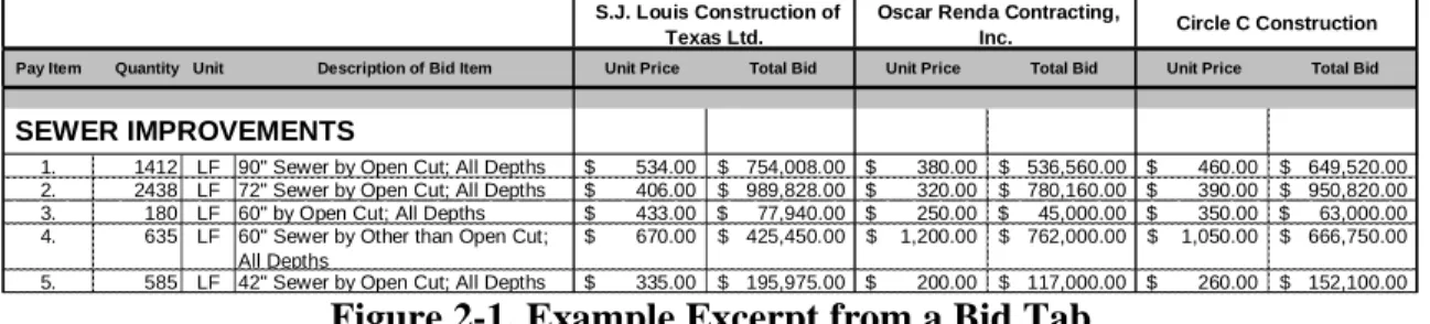
For this study, all 140 bid tabulations recorded between October 2004 and May 2008 were obtained from the City in Excel format; the digital files are provided in a CD inAppendix A. An excerpt from a typical bid tab is shown in Figure 2-1.

(29)

S.J. Louis Construction of Texas Ltd.

Oscar Renda Contracting, Inc.

Pay Item Quantity Unit Description of Bid Item Unit Price Total Bid Unit Price Total Bid Unit Price Total Bid

1. 1412 LF 90" Sewer by Open Cut; All Depths $ 534.00 $ 754,008.00 $ 380.00 $ 536,560.00 $ 460.00 $ 649,520.00

3. 180 LF 60" by Open Cut; All Depths $ 433.00 $ 77,940.00 $ 250.00 $ 45,000.00 $ 350.00 $ 63,000.00

4. 635 LF 60" Sewer by Other than Open Cut;

All Depths

670.00

$ $ 425,450.00 $ 1,200.00 $ 762,000.00 $ 1,050.00 $ 666,750.00

Circle C Construction

SEWER IMPROVEMENTS

Figure 2-1. Example Excerpt from a Bid Tab

As seen in Figure 2-1, a typical City of Fort Worth bid tab provides data regarding the quantity, unit, unit price bid by each contractor, and total price of each pay item in a project. The variability in the unit costs from the table above is typical for most projects. Depending on market conditions, some contractors may not actually want the job but feel they have to bid in order to be considered for future projects from the city. In addition, there might be an error on the plans for a particular cost item that a contractor sees and identifies as a probable change order, so they adjust their unit prices to obtain the greatest return on the change order while still keeping their lump sum price competitive by lowering other items.

Depending on the project scope, a City of Fort Worth construction project can have water, sanitary sewer, and/or paving and drainage improvement pay items. Pay items associated with each category are grouped under the appropriate units; Unit I: water, Unit II: sanitary sewer, Unit III: paving and drainage (Appendix A). Depending on the project scope, one or more of these units may be present in any bid tab. Each City of Fort Worth construction project is unique and the scope varies greatly from project to project. Typically sanitary sewer, water, or paving and drainage improvements would

(30)

each have between 15 and 40 cost items. A project that has sanitary sewer, water, and paving/drainage improvement aspects in its scope may easily have 100 cost items.

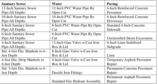
The second step in the UPD development was to decrease the number of cost items to be analyzed to a more manageable size for the purposes of this study. The main pay items that accounted for about 80% of the total cost for sanitary sewer, water, or paving improvements categories were identified. To accomplish this task, three typical candidate projects were randomly identified. The pay items in these candidate projects were sorted by the ratio of their contribution to the total category cost using a Pareto diagram. The identified pay items were further studied, and the items that were not repeatedly used in different projects were eliminated from consideration to be included in the UPD. A cost item was considered not repeatedly used if there were less than 12 occurrences of that item from the bid data. Unit bid price data related to project specific, non-recurring pay items were excluded from this study due to a lack of a sufficient number of data points for analysis. The pay items that account for 80% of the total cost and are repeatedly used in City of Fort Worth sanitary sewer, water, and/or paving projects are presented in Table 2-1.

The third step in the UPD development was to build the framework for the database. Microsoft Excel was selected as the software to house the database. Excel was chosen because of its widespread use amongst the engineers at LGGROUP and many other engineering companies. Furthermore, all of the original bid tabs obtained from the City of Fort Worth were already in Excel format.

(31)

Table 2-1. Pay Items Selected for UPD Development

Sanitary Sewer Water Paving

12-Inch Sanitary Sewer Pipe:All Depths

12-Inch PVC Water Pipe By Open Cut

6-Inch Reinforced Concrete Pavement

6-Inch Reinforced Concrete Driveways

Standard 4-Inch Concrete Sidewalk

6-Inch PVC Water Pipe By Open

Cut Unclassified Street Excavation

12-Inch Gate Valve w/Cast Iron Box & Lid

6-Inch Lime Stabilized Subgrade

Std. 4-feet Dia. Manhole to 6-feet Depth

8-Inch Gate Valve w/Cast Iron

Box & Lid Lime

4-feet Dia. Drop Manhole to 6-feet Depth

6-Inch Gate Valve w/Cast Iron Box & Lid

Temporary Asphalt Pavement Repair

Std. 5-feet Dia. Manhole to

6-feet Depth Ductile Iron Fittings

Permanent Concrete Pavement Repair

Standard Fire Hydrant Assembly

Permanent Asphalt Pavement Repair

Each bid tab essentially provides the same type of information, however the format of the spreadsheets differs depending on the source (consultant engineer or the City personnel) of the original data; therefore it was not possible to combine the separate spreadsheets using an automated (software based) procedure. Instead the data from each bid tab was manually entered into the database framework spreadsheet. The data collected includes the following (Appendix A):

Project Number Number of Bidders Bid Date Contractor Pay Item Quantity Unit Unit Price

(32)

The fourth step was to refine the database by adjusting the unit bid price data from each bid tab to reflect their present day value. Engineering News Record's (ENR) Construction Cost Index was used to adjust the data. For the purposes of this study, the present day was assumed to be December 2008. The database framework was set up to automatically adjust the unit bid prices given any date between October 2004 and present day, thus increasing the robustness of the database and decreasing the effort required to update the spreadsheet every year. The digital UPD excel file is provided in Appendix H.

Summary

The development of the UPD began with separating the cost items into one of three units; Unit 1 for water, Unit 2 for sanitary sewer, and Unit 3 for paving. Using three randomly selected projects from each category, the cost items that typically account for 80% of the total cost for water, sanitary sewer, and paving projects, respectively, were determined. From those items, the ones that occurred 12 times or less where excluded from the UPD since they did not have a large enough sample size for analysis. The items from each bid tab that met the criteria of typically contributing towards 80% of the total construction cost and occurring on at least 12 projects where then entered by hand into the Microsoft Excel UPD. The UPD was set up to automatically adjust the entered data to the present day value using the ENR Construction Cost Index.

(33)

CHAPTER III

STATISTICAL MODEL DEVELOPMENT

As part of the internship objectives, a statistical model was developed for each selected pay item. To develop a statistical model from the compiled unit bid price data, it can be assumed that each pay item constituted a small sample obtained from a larger imaginary population. The imaginary population can be described as being formed by an infinite number of contractors bidding on projects leading to an infinite number of bid prices for each pay item. The unit bid price data gathered in this study represent a smaller sample of that population.

In the internship proposal, it was stated that preliminary results indicated the log-normal probability distribution provided the best fit to model the unit bid price distribution for each pay item. However, further investigation showed that for some of the pay items, normal distribution was a better fit. This study made use of both normal and log-normal distribution to model the unit bid price data collected from the City of Fort Worth.

Developing Histogram Charts

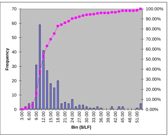
The first step in developing statistical models was to develop histogram charts for each of the pay items. The generated histograms for each item are presented in Appendix B. The histograms for most of the pay items selected indicated a resemblance for log-normal probability distribution as shown in Figure 3-1.

(34)

0 10 20 30 40 50 60 70 3.00 6.00 9.00 12.00 15.00 18.00 21.00 24.00 27.00 30.00 33.00 36.00 39.00 42.00 45.00 48.00 51.00 Bin ($/LF) Fr equ ency 0.00% 10.00% 20.00% 30.00% 40.00% 50.00% 60.00% 70.00% 80.00% 90.00% 100.00%

Figure 3-1. Temporary HMAC Pavement Repair Unit Price Data Histogram

On the other hand, some pay items such as the ones listed below indicated a resemblance for normal probability distribution:

Lime for Stabilization All Size Gate Valves

Ductile Iron Fittings (Figure 3-2) Sanitary Sewer Manholes

(35)

0 5 10 15 20 25 30 35 40 45 50 $400 $2,000 $3,600 $5,200 $6,800 $8,400 More Bin F requ ency

Figure 3-2. Ductile Iron Fittings Unit Price Data Histogram

Coefficient of Variation Effect

Since a small coefficient of variation typically leads to a more symmetrical probability density function, the data appears to be normally distributed. Conversely a larger coefficient of variation leads to an asymmetrical distribution that appears to be log-normal probability distributed. The items that have smaller coefficients of variation tend to be items that do not require much labor, and the items that have a lager coefficient of variation require more labor. In addition, the items with smaller coefficients of variation also have few suppliers in the area, so the cost to the contractors to obtain these items is relatively equal.

(36)

Developing Cumulative Probability Distribution Charts

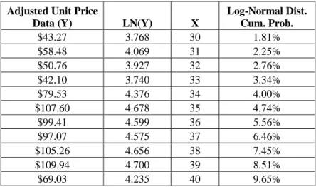
The second step was to develop cumulative probability distribution charts for each of the cost items. To simplify the analysis, each cost item’s unit price data with a histogram that resembled log-normal distribution was transformed by taking the natural logarithm of all the data points; thus making the transformed data set normally distributed. The mean and standard deviation of the transformed data set for each cost item was calculated. These values were used to develop cumulative probability distribution charts. All of these calculations were performed in Excel. A separate tab under each (paving, water, sanitary sewer) database was created for each pay item. An excerpt from the statistical analysis table for 12-Inch Water Line is presented in Table 3-1. The statistical analysis tables for all of the pay items are included inAppendix C.

Table 3-1. Excerpt from the 12-Inch WL Statistical Analysis Table

Adjusted Unit Price

Data (Y) LN(Y) X

Log-Normal Dist. Cum. Prob. $43.27 3.768 30 1.81% $58.48 4.069 31 2.25% $50.76 3.927 32 2.76% $42.10 3.740 33 3.34% $79.53 4.376 34 4.00% $107.60 4.678 35 4.74% $99.41 4.599 36 5.56% $97.07 4.575 37 6.46% $105.26 4.656 38 7.45% $109.94 4.700 39 8.51% $69.03 4.235 40 9.65%

(37)

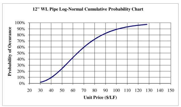
Using the statistical analysis tables, cumulative probability distribution charts were developed for each of the cost items. The log-normal cumulative probability chart for 12-Inch water line is shown in Figure 3-3.

0% 10% 20% 30% 40% 50% 60% 70% 80% 90% 100% 20 30 40 50 60 70 80 90 100 110 120 130 140 150 Probab ility of O ccu ranc e Unit Price ($/LF)

12" WL Pipe Log-Normal Cumulative Probability Chart

Figure 3-3. 12-Inch WL Unit Price Log-Normal Cumulative Probability Chart

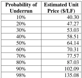
The resulting probability ofunderrun vs.estimated unit price for the 12-Inch WL cost item is presented in Table 3-2. The generated probability charts and tables for all studied pay items are included inAppendix D.

(38)

Table 3-2. 12-Inch WL Probability of Underrun Table Probability of Underrun Estimated Unit Price ($/LF) 10% 40.30 20% 47.27 30% 53.03 40% 58.51 50% 64.14 60% 70.31 70% 77.57 80% 87.03 90% 102.09 98% 135.08

The quantity of each bid item was not dealt with during these calculations, but is addressed in a later section.

Summary

The first step in the statistical model development was to create a histogram of each cost item to determine if it was normally distributed or log-normally distributed. Typically a smaller coefficient in variation led to a normally distributed histogram, and a larger coefficient in variation led to a log-normal probability distributed items. The calculated mean and standard deviation for each cost item were used to create the cumulative probability distribution charts. A tab for each cost item was created in each database (paving, water, and sanitary sewer), and a chart for each was included in Appendix D.

(39)

CHAPTER IV

DECISION MAKING MATRIX DEVELOPMENT

A decision making matrix was developed to provide guidance for selecting an appropriate probability of under run for each analyzed construction cost item. Before a decision making matrix could be developed, the variables that are perceived to influence a contractor’s unit bid price for a given item had to be identified and given a degree of impact on the project. The degree of impact for each variable is assigned an impact rate multiplier that allows each variable to have a different rate of impact on the unit bid prices. To accomplish these tasks, a list of variables from the literature review were selected and presented to the LGGROUP project managers.

Creating the Decision Making Matrix

Ogunlana and Thorpe [32] present several variables that may affect estimating accuracy in their paper. The variables presented by Ogunlana and Thorpe are discussed below:

Type of Project: The type of construction (i.e. a water line construction versus a storm sewer and road reconstruction) in addition to the complexity of the work, the known versus unknown variables (i.e. underground conditions), the number of potential stakeholders involved, and conflicting utilities all may lead to changes in the unit bid prices.

(40)

Size of Project: The size of the project was related to the item quantities since larger project would typically have larger quantities of the items that make up 80 percent of the total construction cost. Item quantity is inversely related to the unit bid price for that item [32].

Geographical Location of Project: Since this study focused on the City of Fort Worth only, this variable does not apply and was excluded from further discussion.

Number of Bidders: The number of bidders is typically inversely related to the unit bid prices. “Also, the statistics of bid distribution ensure that low bids are more likely as the number of bidders increases.” [32] Although the contractors can not know the exact number of bidders an advertised project would generate before the bid documents are opened, they do know the interest the project receives from other contractors before they submit their bids because any interested parties who procure a project set of plans and specifications must sign a list that is public information. This competition is reflected in the average number of bidders for each project.

State of the Market: Current market condition was assessed as the recent national and/or state wide status of the construction industry. “The view in the construction literature is that contractors will be willing to undertake less attractive projects, sometimes at a loss, in periods of low market activity. Conversely, tender levels are expected to rise and competition become more lax in periods of boom.” [32]

(41)

Level of Information Available: This was analyzed as the quality of the plans and specifications which can be measured as the ease or difficulty a project could be constructed as detailed in the plans and specifications. It was assumed that a good clear set of plans and specifications would enable the contractor to have a better understanding of the project, thus lowering the unit bid price. Conversely, a lower quality set of plans and specifications would cause a contractor to add more than required contingency to their cost estimates; thus raising the unit bid price. [32]

Ability of the Estimator: Since this variable is not an area that the engineer has any input on or ability to determine, it was not a measurable variable and eliminated from this study.

Project Duration: Project schedule has an inverse relationship with unit bid prices. If a project is advertised with a shorter than normal construction duration, traditionally the received unit bid prices tend to be higher. A short construction duration would force the contractor to increase the project workforce and this increase in workforce size often results in decreased productivity, thus forcing the contractor to increase his/her unit bid prices to compensate for the loss of productivity. Moreover, if a project has a longer than normal allowed construction duration, the contractor would have the flexibility to move crews between projects, thus decreasing his/her overall operating expenses. The contractor would have the means to lower his/her unit bid prices due to this decrease in expenses. [32]

(42)

These variables were compiled to create the survey forms found in Appendix E. The LGGROUP project managers were asked to complete the surveys to determine the variable impact as detailed in the following section. At this time, the project managers were also able to identify any additional variables they felt should be added to the surveys.

Variable Impact Determination

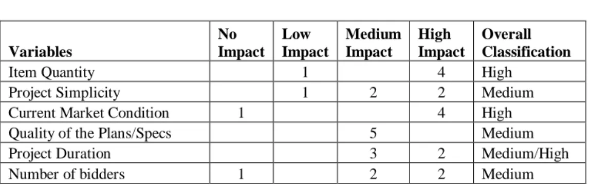
Upon receipt of the survey forms, each project manager was asked to estimate the impact on the unit bid price by those variables previously identified and included on the survey form. The project managers surveyed total approximately 150 years of experience working in the City of Fort Worth on the types of projects included in this project. The surveys by the 5 project managers are presented in Appendix E. The results of the survey are summarized in Table 4-1.

In general, the majority of the variables received similar impact ratings from the project managers, with the exception of theitem quantity andcurrent market conditions, which one project manager disagreed on. The project manager that did not think the item quantity and current market conditions affected the unit bid price had the least amount of experience in the City of Fort Worth (2 years). Because the project managers surveyed represent a large number of years of experience and types of projects, the overall classification ignored the lone outlier and focused on the majority’s opinion. Based on the results of the survey, the factors potentially affecting unit bid prices were categorized into three classification groups regarding their perceived impact on a

(43)

construction item unit bid price; high impact, medium impact, and low impact as shown in Table 4-1.

Table 4-1. Summary of Survey Results

Variables No Impact Low Impact Medium Impact High Impact Overall Classification

Item Quantity 1 4 High

Project Simplicity 1 2 2 Medium

Current Market Condition 1 4 High

Quality of the Plans/Specs 5 Medium

Project Duration 3 2 Medium/High

Number of bidders 1 2 2 Medium

Item quantity andcurrent market condition were estimated to have high impacts on the corresponding unit bid prices. Project duration was identified to have a medium/high impact; project simplicity, quality of plans/ specs, and number of bidders were determined to have medium impacts on the corresponding unit bid prices.

Impact Rate Multiplier Development

To quantify the rate of impact each variable has on the unit bid price, a numerical impact rate multiplier was assigned to each variable based on the rating classification. Each impact rating identified by the project managers had a corresponding numerical multiplier assigned to it as presented in Table 4-2.

(44)

Table 4-2. Impact Rate Multipliers

Variables Impact Rate Multiplier

Item Quantity High 4

Project Simplicity Medium 2

Current Market Condition High 4

Quality of Plans & Specs Medium 2

Project Duration Medium/High 3

Competition (# of bidders) Medium 2

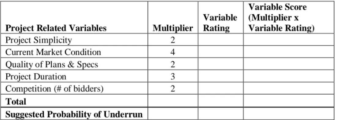
Using the variables and the impact rate multipliers, a decision making matrix was developed for selecting the appropriate probability of under run in order to estimate the unit bid price for a construction item as shown in Table 4-3.

Table 4-3. Blank Decision Making Matrix for Selecting Probability of Under-run

Project Related Variables Multiplier

Variable Rating Variable Score (Multiplier x Variable Rating) Project Simplicity 2

Current Market Condition 4

Quality of Plans & Specs 2

Project Duration 3

Competition (# of bidders) 2

Total

Suggested Probability of Underrun

Determining Probability of Underrun with the Decision Making Matrix

For each construction item, the project managers should fill out the form presented in Table 4-3 to determine the appropriate probability of underrun given the project related variables and item quantity adjustment. Item quantity was separated from other variables because all of the remaining variables would have the same score for a

(45)

given project. In other words, project simplicity, current market condition, quality of plans/specs, project duration, and competition have the same scores for each construction item in a project. However, the score for the item quantity adjustment can vary for each cost item within the project. With this format, the project managers only have to fill out one base form for each project and enter the item quantity adjustment for each cost item.

Each variable that has an impact on the unit bid price of a pay item as defined in this study has an inverse relationship with the unit bid price; for example, a lowerquality of plans/specs should yield a higher unit bid price, or a higherrate of competition should yield a lower unit bid price.

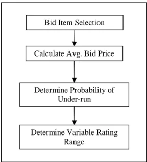
Variable Rating Determination

The next column in the decision making matrix is the variable rating. The values for the variable ratings where determined by analyzing the applicable pay items from the Improvements for Martha and Malinda Project. The conceptual design report [33] that was submitted to the City before the design effort commenced is presented in Appendix F. The report outlines all the infrastructure problems in the project area and how LGGROUP planned to address the issues with the design improvements.

This project was selected because it presented several advantages over other candidate projects, the most important being that the project scope contained improvements for water, sanitary sewer, and paving and drainage. Therefore a large number of cost items that were in the Unit Price Database were also included in the bid

(46)

Bid Item Selection

Calculate Avg. Bid Price

Determine Probability of Under-run

Determine Variable Rating Range

characteristic to a typical City of Fort Worth project in that the main scope was to provide infrastructure improvements to an older part of the City. Since the older parts of the City tend to have more infrastructure problems, the City generally spends more public works’ funds in those areas.

The variable rating determination process is summarized as a flowchart in Figure 4-1.

(47)

The first task for determining the variable rating range was to identify the Martha and Malinda cost items that were included in the UPD. The second step in the process was to calculate the average bid price for each selected cost item. The third step was determining the probability of underrun for each selected pay item that corresponded to the calculated average bid price using the probability charts and tables that were included inAppendix D. For example, the average bid price for 8” PVC Water Pipe in the Martha and Malinda project is $41.83. Based on the probability charts and tables that are included in Appendix D, this corresponds to an average bid probability of underrun of 55%. The result of this analysis is summarized in Table 4-4.

(48)

Table 4-4. Variable Rating Determination Analysis Summary

Description of Item Units Quantity Conatser McClendon JLB Stabile& Winn Avg. Bid Price Avg. Bid Prob. Underrun UNIT COST UNIT COST UNIT COST UNIT COST UNIT COST 8" PVC Water Pipe LF 1,132 $36.00 $41.00 $46.30 $44.00 $41.83 55% 10" PVC Water Pipe LF 1,785 $40.00 $62.00 $67.65 $65.00 $58.66 75%

Temp. Asph. Pavm. Repair LF 3,450 $9.00 $12.00 $13.50 $12.00 $11.63 40%

4" PVC SS Pipe LF 1,075 $35.00 $14.00 $15.95 $13.00 $19.49 30%

8" PVC SS Pipe LF 1,075 $50.00 $51.00 $55.50 $53.00 $52.38 55%

Std. 4' Dia. SSMH (0-6') EA 16 $1,600.00 $3,100.00 $3,370.00 $3,500.00 $2,892.50 75%

Unclassified Street Excavation CY 3,668 $12.50 $17.00 $16.35 $20.00 $16.46 40%

Lime for Subgrade (30 Lbs./SY) TN 173 $110.00 $87.50 $104.00 $110.00 $102.88 15%

6" Lime Stabilized Subgrade SY 11,523 $3.00 $1.75 $2.26 $1.75 $2.19 20%

6" Reinforced Conc. Pavm. SY 10,096 $32.50 $23.50 $28.21 $31.09 $28.83 25%

6" Reinforced Conc. Drive SF 7,151 $6.00 $5.00 $5.34 $5.50 $5.46 30%

Cast Iron/Ductile Iron Fittings TN 4 $3,000.00 $4,000.00 $4,500.00 $4,600.00 $4,025.00 40% Std. 4' Dia. Drop SSMH (0-6') EA 4 $2,000.00 $5,100.00 $5,600.00 $5,800.00 $4,625.00 70%

6" PVC SS Pipe LF 170 $40.00 $49.00 $53.00 $51.00 $48.25 55%

Standard Fire Hydrant EA 2 $1,600.00 $2,500.00 $2,800.00 $2,800.00 $2,425.00 70%

12" PVC Water Pipe LF 60 $45.00 $75.00 $77.50 $76.00 $68.38 60%

(49)

A histogram showing the calculated average bid probability of underrun (POU) values is presented as Figure 4-2. As shown in Figure 4-2, the calculated POU values were within the 15-80 percent range, with an average POU value of 50 percent.

Figure 4-2. Martha & Malinda Calculated POU Histogram

After analyzing the Martha and Malinda project, the variables ratings for each project related variable were determined to be:

Low = 15 Medium = 20 High = 25

Therefore, the project manager rates each project related variable by entering a variable rating where low=15, medium=20, and high=25 depending on the project

0 1 2 3 4 5 6 5% 20% 35% 50% 65% 80% More Bin F re.

(50)

characteristics. For example, a project with a good set of “Plans and Specifications” would have a variable rating of “high=25” in the decision making matrix.

In order to use the Decision Making Matrix (Table 4-3) to determine the probability of underrun, the project manager must determine the variable rating (high, medium, or low) for each project related variable and enter it into the table. The variable score is then determined by multiplying the variable rating by the multiplier for each project related variable. Then, the suggested probability of underrun is calculated by dividing 130 by the total variable scores. The suggested probability of underrun is calculated before quantity adjustment, so that in the worst case scenario where each variable is assigned a low quantity adjustment score, the probability of underrun would be 75 percent. On the other hand, if all the variables are assigned a high quantity adjustment score, the probability of underrun would be 35 percent. The range of the probability of underrun varies by 20 percent from an average of 55 percent based on the difference in bid prices determined by the quantity variable rating which is discussed in further detail in the following section.

Decision Making Matrix Quantity Adjustment

The first step in determining the quantity adjustment was to estimate the quantity variable rating for each selected bid item. The quantity variable rating categorizes the quantity of each bid item into a high, average, or low range. As previously mentioned, the quantity of each bid item has a high impact on the bid price [32]. The objective of this step was to quantify the impact of the bid item quantity on the bid price. The data stored in the UPD was used in the quantity variable rating analysis.

(51)

Estimate Quantity Variable Rating

As part of the quantity variable rating analysis, bid item quantity scatter plot graphs for each cost item were developed using Excel. As an example, the scatter plot for “6-Inch Concrete Driveway” is provided in Figure 4-3.

6" Concrete Driveway Quantity Analysis Scatter Plot 0 5000 10000 15000 20000 25000 30000 0 5 10 15 20 25 30 Project # Q u a n ti ty y (S .F .)

Figure 4-3. 6-Inch Concrete Quantity vs. Project Scatter Plot

A review of the scatter plots and histograms generated for each cost item revealed that the probability distribution that best resembled the bid quantity probability distribution was normal distribution. A cumulative normal distribution function was generated for each cost item in order to determine the high, average, and low quantity ranges. The normal cumulative distribution curve for 6-inch Concrete is shown in

(52)

Figure 4-4. The scatter plots and the log-normal cumulative distribution curves for each cost item are provided inAppendix G.

6" Conc. Pvmt. 0% 10% 20% 30% 40% 50% 60% 70% 80% 90% 100% 0 5000 10000 15000 20000 25000 30000 QUANTITY (LF) NO RM A L CUM . P RO B.

Figure 4-4. 6-Inch Concrete Normal Cumulative Distribution Curve

For the purposes of this study, a low quantity range was defined as any amount that would fall between 0 to 20 percent cumulative probability of occurrence. Quantities higher than 60 percent cumulative probability would be categorized as high. Quantities that fall in between 20 to 60 percent cumulative probability are labeled as average quantities. The results of the quantity analysis are summarized in Table 4-5.

(53)

Table 4-5. Quantity Analysis Results Matrix

Description of Item Units Low Average High

PVC SS Combined L.F. 0-110 110-750 750+

Std. SSMH Combined Sizes Each 0-3 3-9 9+

6" Concrete Pavement S.Y. 0-4000 4000-9000 9000+

6" Concrete Driveway S.F. 0-400 400-4300 4300+

4" Concrete Sidewalk S.F. 0-800 800-7100 7100

Unclassified Street Excavation C.Y. 0-600 600-2500 2500+ 6" Lime Stabilization S.Y. 0-5600 5600-11000 11000+ Lime for Subgrade Stabilization Ton 0-90 90-170 170+ Temporary Asphalt Pavement Repair L.F. 0-1000 1000-3600 3600+ Permanent Asphalt Pavement Repair L.F. 0-80 80-600 600+ Permanent Concrete Pavement Repair S.Y. 0-80 80-450 450+

PVC WL Combined L.F. 0-75 75-1800 1800+

Cast Iron/Ductile Iron Fittings Ton 0-1 1-4 4+

Standard Fire Hydrant (3'-6" Depth) Each 0-2 2-6 6+

Calibrating the Decision Making Matrix Quantity Adjustment

Again, the Improvements for Martha and Malinda Lane Project was used to calibrate the decision making matrix for the quantity adjustment. As previously stated, this project presented several advantages over other candidate projects in that in included many pay items from the Unit Price Database and represented a typical project from the City of Fort Worth for infrastructure improvements.

Using Table 4-5, a Quantity Value Score (QVS) of 1, 2, or 3 was assigned to each bid item. A QVS of 1 was assigned to a bid item with lower than usual quantity amount, whereas a QVS of 3 was assigned to items with higher than usual amounts bid. A QVS of 2 was assigned to items that had quantities that were perceived to have an average quantity amount. The results of the analysis are presented in Table 4-6.

(54)

Table 4-6. Martha and Malinda Cost Items QVS Analysis

DESCRIPTION OF ITEM UNITS QTY Avg. Bid Price

Avg. Bid

POU QVS

8" PVC Water Pipe LF 1,132 $41.83 55% 2

10" PVC Water Pipe LF 1,785 $58.66 75% 2

Temp. Asph. Pavm. Repair LF 3,450 $11.63 40% 3

4" PVC SS Pipe LF 1,075 $19.49 30% 3

8" PVC SS Pipe LF 1,075 $52.38 55% 3

Std. 4' Dia. SSMH (0-6') EA 16 $2,892.50 75% 3

Unclassified Street Excavation CY 3,668 $16.46 40% 3 Lime for Subgrade (30 Lbs./SY) TN 173 $102.88 15% 3 6" Lime Stabilized Subgrade SY 11,523 $2.19 20% 3 6" Reinforced Conc. Pavm. SY 10,096 $28.83 25% 3

6" Reinforced Conc. Drive SF 7,151 $5.46 30% 3

Cast Iron/Ductile Iron Fittings TN 4 $4,025.00 40% 2

Std. 4' Dia. Drop SSMH (0-6') EA 4 $4,625.00 70% 1

6" PVC SS Pipe LF 170 $48.25 55% 2

Standard Fire Hydrant EA 2 $2,425.00 70% 2

12" PVC Water Pipe LF 60 $68.38 60% 1

Perm. Asph. Pavm. Repair LF 35 $69.75 80% 1

Determine Correlation between Probability of Underrun and Quantity Variable Rating

The final step in the matrix calibration process was to determine if there would be a correlation between Probability of Underrun (POU) and the QVS for the selected bid items. A scatter plot graph of QVR versus POU for the Martha and Malinda Project bid items is presented in Figure 4-5.

(55)

POU vs. QFS y = -0.3042Ln(x) + 0.7034 R2 = 0.4137 0% 10% 20% 30% 40% 50% 60% 70% 80% 90% 0 1 2 3 4 QFS POU

Figure 4-5. POU vs. QVS Scatter Plot

As shown in Figure 4-5, there is a negative correlation between POU and QVS. As indicated by the logarithmic best fit equation, a low or high quantity amount compared to an average quantity for a bid item, results in about a 20 percent difference in bid prices. As a result, the POU calculated by a Project Manager using the decision making matrix can be adjusted up to 20 percent depending on the bid item quantity. This 20 percent variance influenced the decisions made previously in regards to the variable rating determination such that the range of probability of underrun was contained within the 35-75 percent range.

(56)

Summary

The decision making matrix was developed to provide the project managers with a tool to determine the probability of underrun for a project based on several variables determined to have an impact on the bid prices for construction projects. These variables were determined based on literature review and work experience. In addition, the project managers used their experience to determine the rate of impact each variable would have on the probability of under-run, and these impact rates were included in the decision making matrix. The Unit Price Database was used to determine the Quantity Variable Rating for each cost item in the UPD. The decision making matrix was then applied to theImprovements to Martha and Malinda Lane Project to calibrate the values chosen in order to have a range for the probability of underrun between 35 and 75 percent.

(57)

CHAPTER V

UNIT PRICE ESTIMATION MODEL APPLICATION

This Chapter discusses the application of the unit price estimation model to an actual project and comparing the results with the current estimating methods utilized at LGGROUP. The project that was selected as the case study is called, “Rosedale Street Improvements.” The project consists of water and sanitary sewer improvements. The first step in the application process is filling out the decision making matrix, and this process was already discussed in Chapter IV. The second step is to compare the engineer’s original unit price estimate with the estimated unit prices from this methodology and also with the actual average bid prices.

Completing the Rosedale Street Improvements Decision Making Matrix

The project manager in charge of the Rosedale Project was asked to fill out the decision making matrix in Excel so an acceptable probability of underrun could be estimated for each cost item. The filled out decision making matrix for this project is shown in Table 5-1.

The suggested POU before the quantity adjustment for the Rosedale Project was calculated to be 55%. Depending on the quantity adjustment, the POU for a bid item can be 35, 55, or 75 percent. The Rosedale Project cost items that were included in the developed Unit Price Database, their respective quantity factor scores, and selected probability of underrun values are listed in Table 5-2.