Quantitative T1 mapping in cardiomyopathy

(1)

Boston University

OpenBU http://open.bu.edu

Theses & Dissertations Boston University Theses & Dissertations

2014

Quantitative T1 mapping in

cardiomyopathy

https://hdl.handle.net/2144/15333 Boston University

(2)

BOSTON UNIVERSITY SCHOOL OF MEDICINE

Thesis

QUANTITATIVE T1 MAPPING IN CARDIOMYOPATHY

by

OWEN MACLEOD HENDRY B.S., University of New Hampshire, 2011

Submitted in partial fulfillment of the requirements for the degree of

Master of Science 2014

(3)

(4)

Approved by

First Reader

Frederick Ruberg, M.D.

Assistant Professor of Medicine and Radiology

Second Reader

Hernan Jara, Ph.D. Professor of Radiology

(5)

DEDICATION

I would like to dedicate this work to my parents Edward and Joreen for always being supportive of me no matter the situation even if things weren't going my way at the time.

I would also like to thank my Uncle David Hendry for offering constant support throughout my education.

(6)

ACKNOWLEDGMENTS

I would like to thank my two advisors Dr. Frederick Ruberg and Dr. Hernan Jara for helping me through this process and for being willing to fit time in to assist me. I would

also like to thank Dr. Yansong Zhao for graciously sending me the files needed to work with the images and for troubleshooting my problems along the way.

(7)

QUANTITATIVE T1 MAPPING IN CARDIOMYOPATHY OWEN MACLEOD HENDRY

ABSTRACT

Recent advancements in techniques of Cardiac Magnetic Resonance Imaging provide extended quantitative measurements of myocardial T1. Important tissue

characteristics can be tracked noninvasively to allow practitioners to quantify important properties of regional and global myocardium function. Quantification of these T1 measures involves the compilation of multiple images to create a T1 recovery curve, providing a map that estimates the T1 value as an encoded pixel value. After contrast injection, the data is compared with native (no applied contrast agent) T1 to examine myocardial disease involving the interstitium as well as the extracellular volume fraction. Myocardial T1 mapping is an emerging biomarker for quantification of myocardial disease (since an important indicator of heart disease is the expansion of myocardial interstitial space, as is fibrosis).

This paper explores the detection and quantification of cardiac involvement using delayed gadolinium enhancement combined with T1 mapping and myocardial

extracellular volume fraction. It extends the research being conducted on Cardiac sarcoidosis, an important cardiomyopathy. Cardiac sarcoidosis is a multisystem granulomatous disease of unknown etiology. Cardiac MR is able to detect the active, inflammatory phase of the disease as well as the chronic phase where scarring and fibrosis are dominant. The use of gadolinium-based contrast agents improves the ability

(8)

to discriminate ischemic from nonischemic etiologies, owing to different patterns among the various nonischemic cardiomyopathies. Since gadolinium shortens T1 relaxation time, the result is a brighter signal intensity in areas with increased interstitial space on inversion recovery T1-weighted sequences.

The 1.5 Tesla Philips Achieva XR Scanner was used to collect the pre- and post- contrast images from five anonymous patients (subjects), following the MOLLI protocol. These images were stacked and run through MRMap, which creates parametric image maps of the MOLLI data. Data was graphed employing the Gado Partition Coefficient.

(9)

TABLE OF CONTENTS

TITLE………...i

COPYRIGHT PAGE………...ii

READER APPROVAL PAGE………..iii

DEDICATION ... iv

ACKNOWLEDGMENTS ... v

ABSTRACT ... vi

TABLE OF CONTENTS ... viii

LIST OF TABLES ... x

LIST OF FIGURES ... xi

LIST OF ABBREVIATIONS ... xii

INTRODUCTION ... 1

(1.1) Magnetic Resonance ... 2

(1.12) Generating the MR signal... 4

(1.13) Radiofrequency pulses and flip angle ... 5

(1.2) T1 and T2 relaxation ... 8

(1.21) Causes of T1 Relaxation ... 9

(1.22) Importance of the T1 value ... 10

(10)

(1.3) Cardiac Magnetic Resonance Imaging ... 12

(1.31) Extracellular Volume Fraction ... 13

(1.4) Physics of T1 Mapping Techniques ... 13

(1.5) Gold standard biomarkers ... 14

(1.51) T1 Mapping ... 14

(1.52) Native (noncontrast) T1 ... 15

(1.53) T1 Mapping with “Look Locker” Inversion Recovery (LL) ... 15

(1.54) T1 Mapping with Modified Look Locker Inversion Recovery (MOLLI) 16 (1.6) Cardiomyopathies ... 17 (1.61) Ischemic Cardiomyopathy ... 17 (1.62) Hypertrophic Cardiomyopathy ... 18 (1.63) Dilated Cardiomyopathy ... 18 (1.64) Cardiac sarcoidosis ... 19 METHODS ... 22 RESULTS ... 29 DISCUSSION ... 38 REFERENCES ... 40 CURRICULUM VITAE ... 44

(11)

LIST OF TABLES

Table Title Page

1 Proposed diagnostic and therapeutic strategy for cardiac sarcoidosis

21

2 Comparison of typical MOLLI sequence parameters 23

3 Sarcoidosis Subject 1 29 4 Sarcoidosis Subject 2 30 5 Sarcoidosis Subject 3 31 6 7 8 9 10 Sarcoidosis Subject 4 Sarcoidosis Subject 5 Other T1 values

Pre and post contrast T1 statistical analysis ECV statistical analysis

32 33 34 34 37

(12)

LIST OF FIGURES

Figure Title Page

1 T1 relaxation process 7

2 Approximate T1 and T2 tissue relaxation values at 1.5T 11 3 Subject #4 MOLLI pre contrast T1 weighted images 24 4 Subject #4 MOLLI post contrast T1 weighted images 25 5 Subject #4 Pre Contast grey scale from MRMap 26 6 7 8 9 10 11 12 13 14 15 16 17 18

Subject #4 Post Contast grey scale from MRMap Subject Subject #4 ROI drawn through myocardium for T1 value Subject #4 ROI drawn in blood for T1 value of blood ECV calculation formula

Gado Partition Coefficient Plot Sarcoidosis Subject #1 Gado Partition Coefficient Plot Sarcoidosis Subject #2 Gado Partition Coefficient Plot Sarcoidosis Subject #3 Gado Partition Coefficient Plot Sarcoidosis Subject #4 Gado Partition Coefficient Plot Sarcoidosis Subject #5 Subject #1 Pre and post contrast MOLLI T1 map Subject #2 Pre and post contrast MOLLI T1 map Subject #3 Pre and post contrast MOLLI T1 map Subject #4 Pre and post contrast MOLLI T1 map

27 27 28 28 29 30 31 32 33 35 36 36 37

(13)

Figure Title Page 19 Subject #5 Pre and post contrast MOLLI T1 map 37

(14)

LIST OF ABBREVIATIONS

AHA ... American Heart Association ARVC/D ... Arrhythmogenic Right Ventricular Cardiomyopathy/Dysplasia BU ... Boston University CMR ... Cardiovascular MRI CVD ... Cardiovascular disease DCM ... Dilated Cardiomyopathy DE ... Delayed Enhancement ECV... Extracellular Volume FID ... Free Induction Decay HCM ... Hypertrophic Cardiomyopathy LL ... Look Locker MOLLI ... Modified Look Locker Inversion MRI ... Magnetic Resonance Imaging MYO ... Myocardium RCM ... Restrictive Cardiomyopathy RF ... Radiofrequency ROI ... Region of Interest TI ... Inversion Time ... ...

(15)

INTRODUCTION

Cardiovascular disease (CVD) is a class of diseases involving the heart and circulatory system. CVD is the leading threat to human health within the United States and Western World. The American Heart Association estimates that 80 million people in the United States have one or more forms of CVD. As the epidemic of obesity, diabetes, and hypertension grows, 40.5% of the US population is projected to have some form of CVD by 2030. [12]

Cardiovascular disease includes many specific illnesses such as coronary heart disease, heart failure, cardiomyopathies, arrhythmias, stroke, pulmonary and arterial hypertension, valvular heart disease, congenital heart disease, and rheumatic heart disease. Because of the wide array of illness associated with CVD, it is important to determine accurately and noninvasively cardiac function in order to diagnose and treat heart disease. [12] Magnetic resonance imaging (MRI) is a quickly evolving modality that provides noninvasive assessment of cardiac function, morphology, tissue

characterization, and perfusion for patients.

The definition of cardiomyopathies has been evolving as diagnostic technology changes and improves. The cardiomyopathies were formerly classified according to the anatomy and physiology into the following types: dilated cardiomyopathy (DMC), hypertrophic cardiomyopathy (HCM), restrictive cardiomyopathy (RCM),

arrhythmogenic right ventricular cardiomyopathy/dysplasia (ARVC/D), and unclassified cardiomyopathy. [2,5] The current definition and classification of cardiomyopathies

(16)

was proposed by the American Heart Association (AHA) in 2006. The AHA defined it as "cardiomyopathies are a heterogeneous group of diseases of the myocardium

associated with mechanical and/or electrical dysfunction that usually (but not invariably) exhibit inappropriate ventricular hypertrophy or dilation and are due to a variety of causes that frequently are genetic. Cardiomyopathies either are confined to the heart or are part of generalized systemic disorders, often leading to cardiovascular death or progressive heart failure related disability." [3]

Cardiomyopathies are classified into two groups. Primary cardiomyopathies mostly involve the heart and secondary cardiomyopathies are accompanied by other organ system involvement. It is important to establish the exact etiology for correct treatment. Cardiovascular MRI (CMR) is a rapidly evolving technology that has seen huge growth in the use of noninvasive imaging of the heart. Its ability to characterize the myocardial and valvular structures and function makes it essential in the diagnostic process and therapeutic management. [2]

(1.1) Magnetic Resonance

Magnetic resonance is a dynamic technology that allows for an imaging study of the anatomic part of interest and the disease process being studied. A magnetic resonance imaging (MRI) system is made up of three main electromagnetic components: a set of main magnet coils, three gradient coils and an integral radiofrequency transmitter coil. Each coil generates a separate type of magnetic field which, when applied to the patient, together create spatially encoded magnetic resonance signals that are used to form MR images. The three different types of magnetic field are defined as follows.

(17)

A strong, constant magnetic field is generated by the main magnet coils. [11] The patient is positioned for imaging within the central bore of the magnet, where the strength of this field, Bo, defines the operating field strength of the particular MRI system. Bo is

measured in units of Tesla, (T) with 1 Tesla equal to approximately 20,000 times the earth's magnetic field. The most common field strength for cardiac imaging today is 1.5T. A reference coordinate system of three orthogonal axes, x, y and z is used to define the magnetic field direction, with the z axis chosen to be parallel to the direction of Bo. [11]

A gradient magnetic field is generated by the three gradient coils within the main magnet. These can be rapidly switched on and off. Each of these gradient coils

generates a magnetic field in the same direction as Bo but with a strength that changes

with position along the x, y or z directions, depending on which gradient coil is used. This gradient field is superimposed onto the Bo magnetic field so that its strength

increases (or decreases) along the direction of the applied gradient field. The strength of the gradient magnetic field reflects the 'steepness' of its slope and is measured in units of millitesla per meter (mT/m). [11]

A radiofrequency (rf) magnetic field is generated by the rf transmitter coil from within the gradient coil. It has a much smaller amplitude than the other magnetic fields, but oscillates at a characteristic frequency in the megahertz range (hence,

radiofrequency), the value of which is determined by the nominal field strength of the main magnet. The rf field is often referred to as the B1 field. The static magnetic field and

radiofrequency field combine to generate magnetic resonance signals that are spatially localized and encoded by the gradient magnetic fields to create an MR image. For cardiac

(18)

imaging, a separate rf receiver coil placed directly over the chest that is tailored to maximize signal from the heart is normally used to detect the emitted MR signals. [11] (1.12) Generating the MR signal

The chemical origin of the MR signal used to generate images is either from water or fat within the patient's tissue. More specifically, it comes from the hydrogen nuclei made up of a single proton, and water/fat are the most abundant species in living tissue. Contained within free water or lipid molecules, Hydrogen is one of a number of elements whose nuclei exhibit magnetic resonance properties and its natural abundance in the form of water and lipid molecules makes it particularly favorable for imaging. [9] The

Hydrogen nuclei possess an essential property known as nuclear spin that gives rise to a small magnetic field for each proton, known as a magnetic moment. [11] Normally the magnetic moments (spins) are randomly oriented, but with an externally applied Bo field,

they tend to align either toward or against the externally applied magnetic field. An equilibrium state is quickly attained where there is a small excess of spins aligned with the field. This is the more energetically favorable direction of alignment. The excess of proton magnetic moments combines to form a net magnetic field or net magnetization. This is often given the symbol M and at equilibrium it is aligned along the positive z axis (along Bo) with the value, Mo. It is often shown as an arrow or vector. [11]

The size of this net magnetization is one of the key determinants of the maximum signal intensity that can be generated and used to form images. The greater the applied magnetic field strength, Bo, the greater the excess of protons aligned with the magnetic

(19)

In order to generate a MR signal from the net magnetization, the radiofrequency (rf) magnetic field is generated by the integral rf transmitter coil and used to deliver energy to the population of protons. This field is applied at a particular frequency, known as the Larmor frequency, ωo that is determined by the Larmor equation:

ωo=γ × Bo

The constant γ is called the gyromagnetic ratio and has a value of 42.6 MHz/Tesla for the proton. The Larmor frequency is proportional to the strength of the magnetic field and for 1.5 Tesla, the Larmor frequency is approximately 64 MHz. [11] This is also known as the resonance frequency, as the protons only absorb energy (or resonate) at this characteristic frequency. The rf field is normally applied as a short pulse, known as an rf pulse. [9]

(1.13) Radiofrequency pulses and flip angle

Before the rf pulse is activated, the net magnetization, Mo, is at equilibrium. It is aligned

along the z-axis in the same direction as Bo and rapidly rotates When the rf pulse is

switched on, the net magnetization starts to rotate away from the Bo field. The speed of

this rotational motion, known as precession, is also at the Larmor frequency. The movement of the net magnetization away from alignment with Bo is caused by a much

slower rotation around the smaller applied rf field, B1. This oscillating field, B1 is applied

as a rotating field at right angles to Bo in the plane of the x and y axes. [11] As it rotates at

the same frequency as the Larmor frequency, it appears as an additional static field to the rotating net magnetization vector. The net magnetization therefore rotates around both the Bo and the B1 fields. As a result of these two rotations, the net magnetization follows a

(20)

spiral path from its alignment with the Bo field (z-axis) towards a rotational motion in the

plane of the x and y axes. [11]

Net magnetization is the result of the sum of many individual magnetic moments. As the magnetic moments rotate together, they will produce a net magnetization that is rotating as well. The greater the amount of energy applied by the rf pulse, the greater the angle that the net magnetization moves from the Bo field (the z axis). [9] This depends upon

both the amplitude and duration of the pulse. The rf pulse is switched off once the angle of precession has reached a desired value. This is known as the flip angle of the rf pulse. Once the rf pulse has caused the net magnetization to make an angle with the z-axis, it can be split into two parts. One section is parallel to the axis and is known as the z-component of the magnetization, Mz, also known as the longitudinal component. The

other component lies at right angles to the z axis within the plane of the x and y axes and is known as the x-y component of the net magnetization, Mxy, or the transverse

component. [9] The transverse component rotates at the Larmor frequency within the xy plane and as it rotates, it generates its own small, oscillating magnetic field which is detected as an MR signal by the rf receiver coil. [11]

(21)

Figure 1: T1 relaxation process [11]

Figure 1 illustrates the process of T1 relaxation after a 90° rf pulse is applied at

equilibrium. The z component of the net magnetization, Mz is reduced to zero, but then

recovers gradually back to its equilibrium value if no further rf pulses are applied.

Excitation pulses are radiofrequency pulses that generate an MR signal by delivering energy to the hydrogen population, causing the magnetization to move away from equilibrium. A 90° rf excitation pulse delivers just enough energy to rotate the net magnetization through 90° [9] This transfers all of the net magnetization from the z-axis

(22)

into the xy (transverse) plane, leaving no magnetization along the z-axis immediately after the pulse. The system of protons is then said to be 'saturated'. [11] When applied once, a 90° rf pulse produces the largest possible transverse magnetization and MR signal.

The 180° pulse refocuses and is used after the 90° excitation pulse, where the net magnetization has already been transferred into the x-y plane. It flips the direction of the magnetization in the x-y plane through 180° as it rotates at the Larmor frequency. This pulse is used in spin echo-based techniques to reverse the loss of coherence caused by magnetic field in homogeneities. [11] The 180° pulses are also used to prepare the net magnetization before the application of an excitation pulse. These are known as inversion pulses and are used in inversion recovery or dark-blood pulse sequences. [11]

(1.2) T1 and T2 relaxation

Immediately after the rf pulse, the system begins to return to equilibrium. This is known as relaxation. There are two relaxation processes that relate to the two components of the Net Magnetization, the longitudinal (z) and transverse (xy) components.

Longitudinal relaxation, known as T1 relaxation is responsible for the recovery of the z component along the longitudinal (z) axis to its original value at equilibrium. [4,7] The second relaxation process, transverse relaxation (T2), is responsible for the decay of the xy component as it rotates about the z axis, causing a subsequent decay of the MR signal. Longitudinal and transverse relaxation both occur at the same time, however, transverse relaxation is typically a much faster process for human tissue. [11]

(23)

(1.21) Causes of T1 Relaxation

T1 is also known as spin-lattice relaxation time and describes how quickly the longitudinal magnetization recovers to its equilibrium. Re-growth of longitudinal relaxation requires a net transfer of energy from the nuclear spin system to its environment (“lattice”) [16]. Because T1 relaxation requires an energy switch, and because all MR energy exchanges must be stimulated, T1 relaxation only can occur when a proton encounters another magnetic field fluctuating near the Larmor frequency. [16] The source of this fluctuating field is usually another proton or electron, and the

interaction is known as a dipole-dipole interaction. [16] In order for a proton or electron to produce a fluctuating magnetic field to cause the T1 relaxation, the molecule in which it resides must be tumbling. The molecule must be rotating near the Larmor frequency to cause T1 relaxation well. Thus, the tumbling rate of the molecule can affect the T1 relaxation time significantly. Small molecules like water tumble too quickly to cause effective T1 relaxation. However, when the water is in a partially bound or restricted state, as it is briefly bonded to proteins and other macromolecules, its tumbling rate may be slowed to a speed near the Larmor frequency. This makes the T1 value of free water very long and the “bound” water is much shorter [16].

The magnetic field strength affects the T1 of different molecules in a different way. For protons in highly mobile molecules (such as free water), the T1 value changes very little because the fraction of protons precessing at Larmor frequency is not altered appreciably. For protons in molecules with intermediate or low mobility, the T1 will

(24)

increase at higher field strength as the fraction of protons decreased significantly at higher Larmor frequency. [3,10]

(1.22) Importance of the T1 value

T1 relaxation is an exponential process with a time constant T1. The shorter the T1 time constant, the faster the relaxation process and return to equilibrium. Recovery of the z-magnetization after a 90° rf pulse is known as saturation recovery. T1 relaxation involves the release of energy from the proton spin population as it returns to its equilibrium state. [11] The rate of relaxation is related to the rate at which energy is released to the surrounding molecular structure. This in turn is related to the size of the molecule that contains the hydrogen nuclei and in particular the rate of molecular motion, known as the tumbling rate of the particular molecule. As molecules tumble or rotate they give rise to a fluctuating magnetic field which is experienced by protons in adjacent molecules. When this fluctuating magnetic field is close to the Larmor frequency, energy exchange is more favorable. Lipid molecules are of a size that gives rise to a tumbling rate which is close to the Larmor frequency and therefore extremely favorable for energy exchange. Fat therefore has one of the fastest relaxation rates of all body tissues and therefore the shortest T1 relaxation time. Larger molecules have much slower tumbling rates that are unfavorable for energy exchange, giving rise to long relaxation times. For free water, its smaller molecular size has a much faster molecular tumbling rate which is also unfavorable for energy exchange and therefore it has a long T1 relaxation time. The tumbling rates of water molecules that are adjacent to large macromolecules can however

(25)

be slowed down towards the Larmor frequency, shortening the T1 value. Water based tissues with a high macromolecular content like muscle therefore tend to have shorter T1 values. Conversely, when the water content is increased, for example by an inflammatory process, the T1 value also increases.

Figure 2: Approximate T1 and T2 tissue relaxation values at 1.5T [12]

(1.23) T2 relaxation

Transverse relaxation (T2) is the result of the sum of the magnetic moments of an entire population of protons within tissues. The presence of interactions between

neighboring protons causes a loss of phase coherence known as T2 relaxation. [11] Immediately after the rf pulse, they rotate together, so that as they rotate they constantly

(26)

point in the same direction within the xy plane. [11] The angle of the direction they point at any time is known as the phase angle and the spins with similar phase angles are in phase. Over time, the phase angles gradually spread out, there is a loss of coherence and the magnetic moments no longer rotate together. The net sum of the magnetic moments is thus reduced, resulting in a reduction in the measured net (transverse) magnetization. The signal that the receiver coil detects if no more rf pulses or magnetic field gradients are applied is therefore seen as an oscillating magnetic field that gradually decays called Free Induction Decay (FID). [11].

(1.3) Cardiac Magnetic Resonance Imaging

Cardiac magnetic resonance (CMR) is evolving into the imaging modality of choice for differentiating the etiology of cardiomyopathies. In comparison to other imaging modalities such as X-ray fluoroscopy, computed tomography, and ultrasound, MRI provides excellent spatial resolution and soft tissue contrast without radiation exposure. [10,16] By using different pulse sequences and acquisition parameters, MRI allows us to examine myocardial function, morphology, perfusion, valvular function, myocardial tissue characterization and so on. Given its enhanced spatial resolution, improved tissue characterization, and lack of ionizing radiation, MRI has become the best choice in the evaluation of patients with cardiomyopathy of unknown etiology. The use of gadolinium based contrast agents can further improve the ability of MRI to

discriminate ischemic from non ischemic etiologies owing to different hyper enhancement patterns among the various non ischemic cardiomyopathies. [10,16]

(27)

Delayed enhancement (DE) MRI (also termed late gadolinium enhancement or hyper-enhancement) defines areas of myocardial fibrosis by imaging 10–15 minutes after gadolinium contrast is administered to the patient. Delayed gadolinium retention in the interstitial space is increased in conditions with increased extracellular volume of distribution and/or decreased washout such as acute necrosis, fibrosis, infiltration and inflammation [10]. Since gadolinium shortens T1 relaxation time, the result is a brighter signal intensity in the areas with increased interstitial space on inversion recovery T1- weighted sequences [3,10]. The presence of delayed enhancement is not specific for any cardiomyopathy though. It is the pattern and location of enhancement that helps in diagnosis and differentiates the diverse etiologies of cardiomyopathies. [3,10]

(1.31) Extracellular Volume Fraction

With the addition of a contrast agent, the extracellular volume (ECV) can be estimated. This is a direct measure of the extracellular space, reflecting interstitial disease. This attempts to split the myocardium into its cellular and interstitial

components with estimates expressed as volume fractions. [10,16] The purpose is to evaluate a change in T1 before and after the administration of contrast agent. It is measured as the percent of tissue comprised of extracellular space which is independent of field strength. [10,16] The ECV in the myocardium may be estimated from the concentration of extracellular contrast agent in the myocardium relative to the blood in a dynamic steady state.

(28)

(1.4) Physics of T1 Mapping Techniques Spin-lattice Relaxation Time

Used in the clinical setting, MRI exploits the magnetic property of hydrogen protons in the human body for diagnostic purposes. The term “spin” comes from the quantum mechanical description of MRI. In 1946, Felix Bloch described nuclear MR phenomenon [16]. Bloch assumed that the ensemble of spins could be represented as a net nuclear magnetization (M) behaving according to the laws of classical

electromagnetism. If the spins constituting M interact only with the external magnetic field (B), they will experience a torque given by the vector cross product (M×B) [16]. Because the torque of a system is equal to the time rate of change of its angular

momentum, Bloch presented the motion of M could be a simple precession around B by the equation:

dM / dt = M × γ B + M0 − Mz/T1 - Mxy/T2

If the spins interact with each other and their environment, M will not precess indefinitely around B, but will return to its original alignment with the main magnetic field (B) with the equilibrium magnitude M0. To return back to the equilibrium state, the spin system must release its energy to the environment, which was termed as relaxation by Bloch. [16] Two time constants T1 and T2 were introduced by Bloch to account for the reestablishment of the thermal equilibrium of the nuclear magnetization following an RF pulse. T1 relaxation was assumed following first-order kinetics by Bloch.

(29)

(1.5) Gold standard biomarkers (1.51) T1 Mapping

T1 mapping is a cardiac magnetic resonance method that provides a parametric map in which the T1 value is encoded in each individual pixel. T1 maps result from a series of co-registered images taken at different times of T1 recovery. Myocardial T1 mapping is an emerging biomarker for quantification of myocardial disease. A major indicator of heart disease is the expansion of myocardial interstitial space, usually

through the development of fibrosis. [3] New developments in cardiovascular magnetic resonance in the measurement of the myocardial T1 relaxation time and the extracellular volume (ECV) have the potential to provide a new biomarker in diagnosis of cardiac disease. T1 relaxation time is a magnetic timing parameter depending on the surrounding molecular environment of tissue and the local magnetic field. [10]

(1.52) Native (noncontrast) T1

Native T1 refers to the longitudinal relaxation time (T1) values of a given tissue with no applied contrast agent. Native T1 measures of myocardium allow for

noninvasive detection of biologically important processes which can be used to improve diagnosis, measures of disease severity, and potentially prognosis. [10,16] Native T1 changes indicate the presence of disease due to increased water content or other changes to the local molecular environment. [7] Iron or fat in tissue reduces native T1 while with fibrosis, edema, and amyloidosis native T1 increases. [11]

(30)

(1.53) T1 Mapping with “Look Locker” Inversion Recovery (LL)

Many cardiac pulse sequences have been developed for T1 mapping, which are used to characterize diseased myocardial tissue. The Look Locker method was

developed in 1970 to accelerate the data acquisition process. To calculate T1 more quickly, the inversion recovery curve was sampled multiple times after a single inversion rather than once as in the conventional inversion recovery-spin echo acquisition. The LL method uses a series of small flip angle excitation pulses (7-15°) after an inversion pulse to sample the inversion recovery curve with different inversion times. [16] The time interval between inversion pulses must be long enough to allow magnetization to return to equilibrium.

Although LL is highly useful, it has inaccuracies resulting from the low flip angle RF pulses exciting the magnetization intermittently. This causes them to fail to return to equilibrium magnetization before the next inversion pulse, often making the T1 values underestimated. [16] Because the images are acquired continuously throughout the cardiac cycle, there is a strong possibility of cardiac motion. Thus, a region of interest (ROI) is required, drawn in an area of the myocardium and moved along with the cardiac motion to calculate T1 in a focal area/lesion of the myocardium. [15,16]

(1.54) T1 Mapping with Modified Look Locker Inversion Recovery (MOLLI) MOLLI was developed in 2004 and is a variant of Look Locker. It is a technique that uses electrocardiogram-gated image acquisition at end-diastole and merges images from multiple consecutive inversion-recovery experiments into one single data set.

(31)

[10,16] The traditional MOLLI protocol uses three inversion-recovery blocks to acquire 11 images over 17 heartbeats. This may present an issue with patients who have

weakened respiratory function due to cardiac diseases because of the requirement for long breath holds. [10]

(1.6) Cardiomyopathies Myocardial fibrosis

Myocardial fibrosis is characterized by expansion of the myocardial extracellular matrix. Accumulation of interstitial collagen is the main characteristic of pathologic remodeling. This derangement affects electrical and mechanical function. [13] Extracellular collagen, the primary component of the expanded extracellular matrix, blocks electrical conduction, is a major component of lethal ventricular arrhythmia, and hardens the myocardium. While CMR with delayed gadolinium enhancement can distinguish large amounts myocardial fibrosis, it cannot detect the full spectrum of myocardial fibrosis. [15]

(1.61) Ischemic Cardiomyopathy

Ischemic cardiomyopathy is defined as dysfunction of the left ventricle as a result of chronic lack of oxygen due to coronary artery disease. [16] With coronary artery disease, myocardial ischemia may result in hibernation, stunning, and true infarction. Stunned myocardium occurs after an acute ischemic event causing reversible contractile dysfunction. Hibernation refers to chronic contractile impairment secondary to chronic hypoperfusion, where the myocardium is still viable. [15,16] By either percutaneous coronary intervention or coronary artery bypass grafting, viable tissue can be

(32)

revascularized and therefore myocardial contractility of the viable tissue can be improved. [15,16]

On delayed contrast enhanced T1-weighted images, infarcted tissues appear bright owing to retained contrast in the region of infarct with decreased contractile ability apparent on the corresponding cine images. On DE MR images, infarcted myocardium and fibrosis appear as high signal intensity in an area of coronary artery distribution. Since all infarctions start subendocardially and may progress towards epicardium, the subendocardium is always involved. [1,16]

(1.62) Hypertrophic Cardiomyopathy

Hypertrophic cardiomyopathy (HCM) is a primary myocardial disease in which the myocardium becomes abnormally thick or hypertrophied. It is a genetic disorder and is caused by a variety of mutations in genes encoding contractile proteins of the cardiac sarcomere. [16] There are currently 11 mutant genes associated with HCM, most commonly β-myosin heavy chain and myosin-binding protein C. [12] Normal

ventricular septal thickness is around 8-12 mm and in HCM, the diastolic left ventricular wall thickness is 15 mm or more. [13] In HCM, the left ventricular volume can be reduced or normal and diastolic dysfunction is usually seen. Premature death and arrhythmias are often seen in HCM.

Delayed contrast enhanced T1-weighted images typically show patchy, multifocal hyper enhancement in patients with HCM occurring only within hypertrophied areas. It

(33)

is considered that the patchy enhancement is due to the occurrence of abundant connective tissue within the hypertrophic myocardium [15].

(1.63) Dilated Cardiomyopathy

Dilated cardiomyopathy (DCM) is described by ventricular chamber enlargement and impaired function of the left ventricle with a left ventricular ejection fraction less than 40% [13]. The causes of dilated cardiomyopathy is broad and may be idiopathic, familial/genetic, viral and/or immune, alcoholic/toxic. [16]. DCM leads to progressive heart failure and a decline in left ventricular contractile function, arrhythmias, conduction system abnormalities, and sudden death. [16] DCM is a common and largely irreversible form of heart muscle disease. Patients with idiopathic dilated cardiomyopathy show either linear midmyocardial enhancement or no enhancement[10,13]. This enhancement is thought to be due to fibrosis.

(1.64) Cardiac sarcoidosis

Sarcoidosis is defined by the American Thoracic Society as a multisystem granulomatous disease of unknown etiology. A significant contributor of disease development and progression is the individually defined immune response and degree of inflammation, which represents a major target for diagnosis and therapy. Lymph nodes and lungs are most frequently involved, but the disease can affect any other organ and cardiac involvement commonly occurs. Cardiac involvement leads to varied outcomes and ranges from asymptomatic to sudden cardiac death. Cardiac sarcoidosis is

(34)

involved area is the ventricular septum (31.5%), followed by the inferior wall, anterior left ventricle, right ventricle, and lateral left ventricle. [12]

Cardiac MR is able to detect the active, inflammatory phase of the disease as well as the chronic phase where scarring and fibrosis are predominant. [12] The active phase is distinguished by focal wall thickening due to edema (identified by T2-weighted imaging) with wall motion abnormalities seen on cine images and early gadolinium enhancement noted due to excessive capillary leak. The chronic stage mostly shows wall thinning with delayed gadolinium enhancement, representing myocardial damage,

scarring, and fibrosis. [12] The two phases often overlap.

The objective of this study is to utilized advanced T1 studies such as MOLLI and ECV to assess cardiac function in patients with known cardiomyopathy with a focus on cardiac sarcoidosis.

(35)

Table 1: Proposed diagnostic and therapeutic strategy for cardiac sarcoidosis [12] Indications for screening

Diagnosed extracardiac sarcoidosis Unexplained persisting second- or third-degree atrioventricular block and age < 55 y

Unexplained monomorphic ventricular tachycardia Nonischemic dilated cardiomyopathy

Routine screening procedures Findings leading to further work-up Clinical symptoms, physical

examination

12-lead electrocardiogram

Bundle branch block, ventricular ectopy, second- or third-degree atrioventricular block (atrial arrhythmia, first-degree atrioventricular block) Echocardiogram

Global LV dysfunction, regional wall motion abnormalities (right ventricular dysfunction)

Holter monitoring

Runs of ventricular tachycardia, nonsustained ventricular tachycardia (frequent isolated premature ventricular contractions) Further work-up Findings leading to therapy CMR

Delayed hyperenhancement (LV dysfunction, perfusion defects)

PET

Patchy or focal 18F-FDG uptake (patchy on diffuse uptake)

Invasive electrophysiologic study Abnormal result

Therapy Triggered by

Immunomodulation (prednisone

[30–40 mg]; methotrexate Positive further work-up Implantable

cardioverter-defibrillator Positive electrophysiologic study Response evaluation Evidence of efficacy improvement Symptoms

CMR (no implantable

cardioverter-defibrillator) Reduction in T2 signal

(36)

METHODS

The study was approved by the IRB and is HIPPA compliant. The subjects were scanned on a 1.5 Tesla Philips Achieva XR scanner and afterwards had their images anonymized. The sequences used in the optimized cardiac sarcoidosis MOLLI protocol: 1. T1-BB axial (aortic arch to inferior aspect of heart below diaphragm)

2.Horitzonal long axis (SSFP cine) 3. Vertical long axis (SSFP cine) 4. Short axis stack (SSFP cine) 5. 4-chamber stack (SSFP cine) 6. Aortic valve flow

7. Pulmonic valve flow

8. T2-BB in short axis plane with STIR

9. Pre contrast MOLLI 3,3,5 sequence for native T1 map in 3 slices 10. Standard delayed gadolinium enhancement

11. Post contrast (>15 min after injection), MOLLI 3,3,5 in same slices as above)

Prior to scanning the patient, a blood draw is done to assess their hematocrit level, a test that measures the percentage of red blood cells in blood. Normal range for

hematocrit is different between the sexes and is approximately 45% to 52% for men and 37% to 48% for women. [14]

(37)

Table 2: Comparison of typical MOLLI sequence parameters [2]

Sequence Optimized MOLLI sequence Original MOLLI sequence

Preparation Non-selective inversion recovery Non-selective inversion recovery Bandwidth 1090 Hz/px 1090 Hz/px Flip Angle 35° 50° Base Matrix 192 240 Phase resolution 128 151 FOX x %phase 256x100 380 x 342

Inversion Time (TI) 100 ms 100 ms

Slice Thickness 8 mm 8 mm Acquisition window 202 ms 191.1 ms Trigger delay 300 ms 300 ms Inversions 3 3 Acquisition heartbeats 3,3,5 3,3,5 Recovery heartbeats 3,3,1 3,3,1 TI increment 80 ms 100-150 ms

Scan time 17 heartbeats 17 heartbeats

(38)

(39)

Figure 4: Subject #4 MOLLI Post contrast T1 weighted images (1-8)

Gadolinium is hand injected at 1ml/second and is based on the patients weight. Dosage increases 1 mL per every 10 kilograms but is 1.5x the usual dose in cardiac studies. The

(40)

pre and post contrast images are then stacked and run through MRMap which is a

program that creates parametric image maps of the MOLLI data. From there color tables are added to the images based on T1 values in milliseconds.

T1 Maps:

(41)

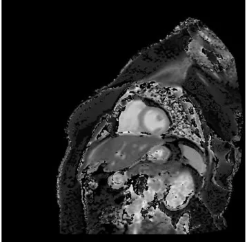
Figure 6: Subject #4 Post Contast grey scale from MRMap

The T1 map is then imported to ImageJ where a region of interest is drawn free hand through the myocardium and within the ventricular blood pool to get T1 values. Figure 7: Subject #4 Region of interest drawn through myocardium for T1 value

(42)

Figure 8: Subject #4 Region of interest drawn in blood for T1 value of blood

The T1 value is then converted into R1 or 1/T1 which is the longitudinal relaxation rate for both pre and post contrast images of the myocardium and blood. The R1 values are then placed on a scatter chart with the Y-axis utilizing the myocardium pre and post contrast values and the X-axis using the blood pre and post contrast values to find the slope. The correction factor is calculated by the equation 1-(Hematocrit/100). The ECV is then measured by multiplying the correction factor by the slope attained in the graph. Figure 9: ECV measurement equation [6]

(43)

RESULTS

Table 3: Sarcoidosis Subject #1

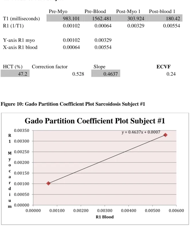
Pre-Myo Pre-Blood Post-Myo 1 Post-blood 1 T1 (milliseconds) 983.101 1562.481 303.924 180.42

R1 (1/T1) 0.00102 0.00064 0.00329 0.00554

Y-axis R1 myo 0.00102 0.00329 X-axis R1 blood 0.00064 0.00554

HCT (%) Correction factor Slope ECVF

47.2 0.528 0.4637 0.24

Figure 10: Gado Partition Coefficient Plot Sarcoidosis Subject #1

y = 0.4637x + 0.0007 0.00000 0.00050 0.00100 0.00150 0.00200 0.00250 0.00300 0.00350 0.00000 0.00100 0.00200 0.00300 0.00400 0.00500 0.00600 R 1 M y o c a r d i u m R1 Blood

(44)

Table and graph for individual subjects listing the T1 values of pre and post contrast myocardium and blood. R1 values listed below the T1 values after calculating (1/T1) for each. The pre and post contrast R1 of myocardium was plotted on the Y-axis while the R1 pre and post contrast of blood was plotted along the X-axis. The slope was derived from the graph. The hematocrit percentage was recorded prior to scanning by a blood draw. Correction factor was measured by 1- (hematocrit / 100). ECV was then

calculated by multiplying the slope by correction factor. Process completed for all other subjects.

Pre-Myo Pre-Blood Post-Myo 1 Post-blood 1 T1 (milliseconds) 996.34 1581.454 343.594 182.28 R1 (1/T1) 0.00100 0.00063 0.00291 0.01 Y-axis R1 myo 0.00100 0.00291 X-axis R1 blood 0.00063 0.00549

1 0.4783 0.48

y = 0.4783x + 0.0003 0.00000 0.00050 0.00100 0.00150 0.00200 0.00250 0.00300 0.00350 0.00000 0.00100 0.00200 0.00300 0.00400 0.00500 0.00600 R 1 M y o c a r d i u m R1 Blood

(45)

R1 (1/T1) 0.000968 0.000605 0.002693 0.004630

27.8 0.722 0.4285 0.31

y = 0.4285x + 0.0007 0.00000 0.00050 0.00100 0.00150 0.00200 0.00250 0.00300 0.00000 0.00100 0.00200 0.00300 0.00400 0.00500 R 1 M y o c a r d i u m R1 Blood

(46)

R1 (1/T1) 0.00103 0.00066 0.00208 0.00426

42.5 0.575 0.2922 0.17

y = 0.2922x + 0.0008 0.00000 0.00050 0.00100 0.00150 0.00200 0.00250 0.00000 0.00050 0.00100 0.00150 0.00200 0.00250 0.00300 0.00350 0.00400 0.00450 R 1 M y o c a r d i u m R1 Blood

(47)

R1 (1/T1) 0.00100 0.00066 0.00210 0.00405

34.6 0.654 0.3227 0.21

y = 0.3227x + 0.0008 0.00000 0.00050 0.00100 0.00150 0.00200 0.00250 0.00000 0.00050 0.00100 0.00150 0.00200 0.00250 0.00300 0.00350 0.00400 0.00450 R 1 M y o c a r d i u m R1 Blood

(48)

Table 8: Other T1 values from subjects (tissues within field of view) Subject #1 T1 values (ms) Liver Fat

Pre contrast 461 273

Post Contrast 295 282

Subject #2 Liver Fat

T1 values of liver and fat measured from the images processed as a reference to cardiac T1 values. The approximate T1 value at 1.5T for liver is 500 and for fat is 250. Most values fall within this range and slight deviation may be due to artifact affecting the selected ROI mean.

(49)

Table 9: Pre and post contrast T1 statistical analysis Pre contrast myo Post contrast Myo Pre contrast blood Post contrast blood Patient #1 983.101 303.924 1562.481 180.42 Patient #2 996.34 343.594 1581.454 182.28 Patient #3 1032.659 371.334 1651.6 215.97 Patient #4 972.262 480.651 1522.378 234.911 Patient #5 999.316 477.124 1522.153 246.84 Mean 996.736 395.325 1568.013 212.084 SD 22.815 79.965 53.347 30.146

An organized data table collecting all T1 values for pre and post contrast myocardium and blood of all five subjects. Averages were taken of each column and the standard deviation was found for each to evaluate statistical differences among the patients. Figure 15: Subject #1 Pre and post contrast MOLLI T1 map

(50)

Pre and post contrast MOLLI T1 maps post processed with MRMap for each subject. Color added using blue/green/red/yellow color table based off the T1 ms reference range along the left side.

Figure 16: Subject #2 Pre and post contrast MOLLI T1 map

(51)

Figure 18: Subject#4 Pre and post contrast MOLLI T1 map

(52)

Table 10: ECV statistical analysis

ECV values

Patient #1 0.24 Mean ECV 0.282

Patient #2 0.48 SD 0.122

Patient #3 0.31 Patient #4 0.17 Patient #5 0.21

Collection of EVC values of all five patients after calculated by multiplying the slope

by the correction factor, with the average ECV and standard deviation recorded.

DISCUSSION

The objective of this study was to utilize advanced T1 studies to assess cardiac function in patients with known cardiomyopathy, with a focus on cardiac sarcoidosis. In general, the normal 'healthy' ECV value ranges from 0.27-0.30 while the average pre contrast myocardium T1 values fall around 950-1000 ms. Using the data obtained from this study, the average of the five subjects' ECV was found to be 0.282 with a standard deviation of 0.122. This high standard deviation was to be expected with a low number of subjects. One subject was well above the normal range, three well below, and one within the range, all previously diagnosed with cardiac sarcoidosis. The native T1 myocardium mean was 996.736 with a standard deviation of 22.815 while the post contrast T1 myocardium mean was 395.325 with a standard deviation of 79.965. The

(53)

native T1 values fell within the correct range. The liver T1 values all decreased after Gadolinium injection while fat T1 mostly stayed the same.

As native T1/post contrast mapping and ECV techniques continue to improve, clinicians will be able to develop further insight into cardiac disease processes that are difficult to evaluate. Recent studies indicate that the occurrence of sarcoidosis and the risk of mortality relating to cardiac involvement have been on the rise over the past several decades. [12] Cardiac sarcoidosis, although an uncommon disease, should be considered in all cases of unexplained cardiomyopathy, especially within younger patients. With the emergence of advanced cardiac imaging, CS is being diagnosed earlier and more frequently than before.

A major limitation to this study was a limited amount of cardiac sarcoidosis patients. Another limitation is the difficult process of reducing cardiac and respiratory motion artifact. In addition to motion artifact, patients with weakened respiratory function may have a difficult time holding their breath long enough during acquisitions. Luckily, patients rarely have adverse effects to the use of Gadolinium which is a requisite of CMR. This procedure can be quite lengthy (45-60 minutes), requiring the patient to remain still longer than many other studies. The partnership of the radiologist and cardiologist is important in determining the extent and pattern of the disease. The information provided through this current research, while somewhat limited to five samples, lends strong support for further exploration of noninvasive diagnostic and prognostic evaluation of this pathology.

(54)

REFERENCES

[1] Elster, Allen D., MD. "Size of T1 vs T2." Questions and Answers in MRI. N.p., 2014. Web. 28 July 2014.

[2] Fernandes, Juliano Lara, Ralph Strecker, Andreas Greiser, and Jose Michel Kalaf. "Myocardial T1-Mapping: Techniques and Clinical Applications." Myocardial T1-Mapping: Techniques and Clinical Applications (n.d.): n. pag. Clinical Cardiovascular Imaging. Siemens Healthcare, Jan. 2012. Web. 28 July 2014.

[3] Heidenreich, Paul A., MD, Justin G. Trogdon, PhD, Olga A. Khavjou, MA, Javed Butler, MD, Kathleen Dracup, DNSc, Michael D. Ezekowitz, DPhil, Eric Andrew Finkelstein, PhD, Yuling Hong, MD, S. Clairborne Johnston, MD, PhD, Amit Khera, MD, Donald M. Lloyd-Jones, MD, Sue A. Nelson, MPA, Graham Nichol, MD, Diane Orenstein, PhD, Peter W.F. Wilson, MD, and Joseph Woo, MD. "Forecasting the Future of Cardiovascular Disease in the United States." A Policy Statement From the American Heart Association. Circulation, Jan. 2011. Web. 28 July 2014.

[4] Higgins, David M., and James C. Moon. "Review of T1 Mapping Methods: Comparative Effectiveness Including Reproducibility Issues." Review of T1 Mapping Methods: Comparative Effectiveness Including Reproducibility Issues. N.p., 01 Jan. 2014. Web. 28 July 2014.

[5] Kaderli, Aysel Aydin, Sumeyye Gullulu, Funda Coskun, Dilber Yilmax, and Ersa Uzaslan. "Impaired Left Ventricular Systolic and Diastolic Functions in Patients with

(55)

Early Grade Pulmonary Sarcoidosis." European Journal of Echocardiography (2010): n. pag. European Society of Cardiology, 23 Apr. 2010. Web. 28 July 2014.

[6] Kellerman, Peter, Joel R. Wilson, Hui Xue, Martin Ugander, and Andrew E. Arai. "Extracellular Volume Fraction Mapping in the Myocardium, Part 1: Evaluation of an Automated Method." Journal of Cardiovascular MR. Journal of Cardiovascular MR, 10 Sept. 2012. Web. 28 July 2014.

[7] Kellman, Peter, and Michael S. Hansen. "T1-mapping in the Heart: Accuracy and Precision." Journal of Cardiovascular MR. Journal of Cardiovascular MR, 4 Jan. 2014. Web. 28 July 2014.

[8] Lee, Jason J., Songtao Liu, Marcelo S. Nacif, Martin Ugander, Jing Han, Nadine Kawel, Christopher T. Sibley, Peter Kellman, Andrew E. Arai, and David A. Bluemke. "Myocardial T1 and Extracellular Volume Fraction Mapping at 3 Tesla." Journal of Cardiovascular MR. Journal of Cardiovascular MR, 28 Nov. 2011. Web. 28 July 2014. [9] Manning, Warren J., and Dudley J. Pennell. Cardiovascular Magnetic Resonance. Philadelphia, PA: Saunders/Elsevier, 2010. Print.

[10] Moon, James C., Daniel R. Messroghli, Peter Kellman, Stefan K. Piechnik, Matthew D. Robson, Martin Ugander, Peter D. Gatehouse, Andrew E. Arai, Matthias G. Friedrich, Stefan Neubauer, Jeanette Schulz-Menger, and Erik B. Schelbert. "Myocardial T1

Mapping and Extracellular Volume Quantification: A Society for Cardiovascular Magnetic Resonance (SCMR) and CMR Working Group of the European Society of

(56)

Cardiology Consensus Statement." Journal of Cardiovascular MR. Journal of Cardiovascular MR, 14 Oct. 2013. Web. 28 July 2014.

[11] Ridgway, John P. "Cardiovascular Magnetic Resonance Physics for Clinicians: Part I." Journal of Cardiovascular MR. SCMR, 30 Nov. 2010. Web. 28 July 2014.

[12] Schatka, Imke, and Frank M. Bengel. "Journal of Nuclear Medicine." Advanced Imaging of Cardiac Sarcoidosis. N.p., 1 Jan. 2014. Web. 28 July 2014.

[13] Schelbert, Erik B., Stephen M. Testa, Christopher G. Meier, William J. Ceyrolles, Joshua E. Levenson, Alexander J. Blair, Peter Kellman, Bobby L. Jones, Daniel R. Ludwig, David Schwartzman, Sanjeev G. Shroff, and Timothy C. Wong. "Myocardial Extravascular Extracellular Volume Fraction Measurement by Gadolinium

Cardiovascular Magnetic Resonance in Humans: Slow Infusion versus Bolus." Journal of Cardiovascular MR. Journal of Cardiovascular MR, 4 Mar. 2011. Web. 28 July 2014. [14] Shiel Jr., William C., MD. "What Is a Normal Hematocrit? - Hematocrit: Learn About Different Test Levels." MedicineNet. MedicineNet, 10 Apr. 2014. Web. 27 July 2014.

[15] Van Es, Wouter, Hans Van Heesewijk, Benno Rensing, Jan Van Der Heijden, and Robin Smithuis. "Ischemic and Non-ischemic Cardiomyopathy." The Radiology

Assistant. The Educational Site of the Radiological Society of the Netherlands, 12 Nov. 2009. Web. 28 July 2014.

(57)

[16] Zhou, Xiaopeng. "Myocardial T1 Mapping Techniques." Myocardial T1 Mapping Techniques. Cleveland State University, Dec. 2012. Web. 28 July 2014.

(58)

CURRICULUM VITAE Owen MacLeod Hendry

YOB: 1988

[email protected]

Education

Boston University School of Medicine, Boston, MA Division of Graduate Medical Sciences

Masters of Science – Bioimaging, August 2014

Thesis Title: Quantitative T1 mapping in cardiomyopathy

University of New Hampshire, Durham, NH College of Life Sciences and Agriculture (COLSA) Bachelor of Science in Biology, May 2011

Imaging Experience

Boston Medical Center, Boston, MA January 2014 to August

2014

Clinical MRI Intern, Radiology Department (outpatient and inpatient)

 Positioning and scanning of adult and pediatric patients using 1.5T Phillips scanners and 3.0T GE scanner environment

(59)

 Communicating with culturally diverse patient populations in a comforting manor to maintain a positive environment

 Transporting patients to and from the MRI suites safely and efficiently  Assisting in work flow of MRI operations

 Maintaining compliance with all MRI safety protocols and regulations  Communicating with staff and radiologists to ensure proper patient care

Catholic Medical Center, Manchester, NH May 2011 to September 2012

Emergency Department medical scribe

 Accurately and thoroughly documented patient visits including patient's history, chief complaint, and physical exam results

 Input physician dictated notes and updates regarding care while in the ED

 Developed an understanding of ordering tests, interpreting lab results, and reading radiologic test results

 Prepared plans for follow-up care

 Gained invaluable clinical experience for health related professional pursuits  See and be a part of the medical decision process

 Mastered electronic medical records

 Learned medical terminology, language and general medical knowledge 

Quirk Chevrolet, Manchester, NH May 2010-September 2010

(60)

 Carried out promotions and sales activities on the internet

 Spoke with prospective customers by phone or email regarding interest in vehicles, potential deals, and any general questions regarding the company

 Organized the Chevrolet website, updating new vehicles and sales  Scheduled appointments with interested buyers

 Developed strong interpersonal skills

Technical Skills

 Utilizing MRMap, 3D Slicer, Image J, MRIcro, MRIcron, MATLAB software for image analysis of DICOMs

 Familiar with 1.5T Phillips scanners and 3.0T GE scanner