Type Inference for First-Class Messages
with Match-Functions
Paritosh Shroff
Scott F. Smith
Johns Hopkins University
{pari, scott}@cs.jhu.edu
Abstract
Messages that can be treated as class entities are called first-class messages. We present a sound unification-based type infer-ence system for first-class messages. The main contribution of the paper is the introduction of an extended form of function called a match-function to type first-class messages. Match-functions can be given simple dependent types: the return type depends on the type of the argument. We encode objects as match-functions and messages as polymorphic variants, thus reducing message-passing to simple function application. We feel the resulting system is sig-nificantly simpler than previous systems for typing first-class mes-sages, and may reasonably be added to a language design without overly complicating the type system.
Keywords
First-class messages, polymorphic variants, object-oriented pro-gramming, constraint-based type inference, unification, object-encoding.
1
Introduction
First-class messages are messages that can be treated as first-class values and bound to program variables. Hence, we can write obj← x, where obj is an object, x a program variable and←represents message passing. Since the message assigned to x can be varied at run-time, we can change the message sent to obj dynamically. This is the exact dual of dynamic dispatch, where we change the object at run-time—here we want to be able to change the message at runtime.
First-class messages are useful in typing delegate objects, which forward messages to other objects. For example, in
let m= fmessage()in
let o1={forward(x) =o2←x}in o1←forward(m)
o1is a delegate object whereforward (x)is the method that delegates, i.e. forwards,xtoo2. fmessage()is the first-class message which gets assigned tom, thenx, and finally forwarded too2. Such del-egate objects are ubiquitous in distributed systems such as proxy servers giving access to remote services (e.g. ftp) beyond a fire-wall. The following is an example of a proxy server cited by M¨uller [MN00]:
let ProxyServer={new(o) ={send(m) =o←m}}
This creates an objectProxyServerwith a methodnewthat receives an object o and returns a second object with a methodsend. send
takes an abstract first-class messagemas a argument and forwards it too. We can create a Ftp proxy server as:
let FtpProxy=ProxyServer←new(ftp)
whereftpis aFtpobject. A typical use of this new proxy is
FtpProxy←send(get(0paper.ps.gz0))
getis a method inftp. Delegation of abstract messages cannot be easily expressed without first-class messages, since the message can be changed at run-time and hence must be abstracted by a vari-ablem. [MN00] and [Nis98] further discuss how first-class mes-sages can exploit locality by abstracting remote computations in distributed object-oriented computing.
Modern typed object-oriented programming languages (e.g. Java, C++) do not support first-class messages. Smalltalk [GR89] and Objective-C [PW91] provide untyped first-class messages. The static type-checking of first-class messages presents two main difficulties:
1. Typing first-class messages that can be placed in variables and passed as values, e.g. m=fmessage(): we need a way to express and type standalone messages.
2. Typing abstract message-passing to objects, such as o←x: since x can be any message in o and these different messages can have different return types, o←x doesn’t have a single return type but rather its type depends upon the type of x. We need to be able to encode its static type such that it depends on the abstract type of x.
We solve the first problem by encoding messages as polymorphic variants which have standalone types, i.e., a polymorphic variant ‘fmessage()has type ‘fmessage().
The second problem is more challenging, and the most important contribution of this paper is the simplicity of its solution. We in-troduce an extended form of function (inspired by SML/NJ’s pat-tern matching functions) called a match-function, which always takes a variant as argument and has a return type that can de-pend on the argument variant. We call these dependent types match-types. We encode objects as match-functions, thus reduc-ing message sendreduc-ing to simple function application. There are sev-eral other solutions to typing first-class messages in the literature [Wak93, Nis98, MN00, Pot00]; the main advantage of our approach is its simplicity.
We organize the rest of the paper as follows. We review OCaml’s polymorphic variants in Section 1.1, and review the duality of
records and variants in Section 1.2. In Section 2 we defineDV, a core language with match-functions. In Section 3 we present a type system forDVthat includes match-types, and show it is sound. In Section 4 we present a constraint-based type inference system for inferring match-types along with an algorithm for simplifying the constrained types to human-readable constraint-free types and prove its soundness. The net result is a type inference algorithm for the originalDVtype system. Section 5 illustrates all aspects of the system with a series of examples. In Section 6 we show how objects with first-class messages can be faithfully encoded with match-functions. Section 7 discusses the related work.
Some portions of the paper aregrayed out. They represent optional extensions to our system which enhance its expressiveness at the expense of added complexity. The paper can be read assuming the
grayportions don’t exist. We recommend the readers skip these grayed out portions during their initial readings to get a better un-derstanding of the core system.
1.1
Review of Polymorphic Variants
Variant expressions and types are well known as a cornerstone of functional programming languages. For instance in OCaml we may declare a type as:
type feeling = Love of string | Hate of string | Happy | Depressed
Polymorphic variants [Gar98, Gar00], implemented as part of Ob-jective Caml [LDG+02], allow inference of variant types, so type declarations like the above are not needed: we can directly write expressions like‘Hate("Fred")or‘Happy.
We use the Objective Caml [LDG+02] syntax for polymorphic vari-ants in which each variant name is prefixed with‘. For example in OCaml 3.07 we have,
let v = ‘Hate ("Fred");;
val v : [> ‘Hate of string] = ‘Hate "Fred"
[> ‘Hate of string] is the type of the polymorphic variant ‘Hate ("Fred"). The “>” at the left means the type is read as “these cases or more’’. The “or more” part means these types are polymorphic, it can match with a type of more cases.
Correspondingly, pattern matching is also given a partially specified type. For example,
let f = fun ‘Love s -> s | ‘Hate s -> s
-: val f : [< ‘Love of string | ‘Hate of string] -> string [< ‘Love of string | ‘Hate of string]is the inferred vari-ant type. The “<” at the left means the type can be read “these cases or less”, and since ‘Hate ("Fred") has type [> ‘Hate of string],f ‘Hate ("Fred")will typecheck. Polymorphic variants are expressible without subtyping, and are thus easily incorporated into unification-based type inference al-gorithms. They can be viewed as a simplified version of [R´89, Oho95].
Our type system incorporates a generalization of Garrigue’s notion of polymorphic variants that explicitly maps the variant coming in to a function to the variant going out. This generalization is useful in functional programming, but is particularly useful for us in that it allows objects with first-class messages to be expressed using only variants and matching, something that is not possible in any of the
existing polymorphic variant type systems above.
1.2
The Duality of Variants and Records
It is well-known that variants are duals of records in the same man-ner as logical “or” is dual to “and”. A variant is this field or that field or that field . . . ; a record is this field and that field and that field . . . . Since they are duals, defining a record is related to using a variant, and defining a variant is like using a record. In a program-ming analogy of DeMorgan’s Laws, variants can directly encode records and vice-versa.
A variant can be encoded using a record as follows: matchswith‘n1(x1)→e1|. . .|‘nm(xm)→em≡
s{n1=funx1→e1, . . . ,nm=funxm→em}
‘n(e)≡(funx→(funr→r.n x))e
Similarly, a record can be encoded in terms of variants as follows: {l1=e1, . . . ,lm=em} ≡
funs→ matchswith‘l1(x)→e1|. . .|‘lm(x)→em where x is any new variable. The corresponding selection encoding is: e.lk≡e ‘lk( )
where could be any value.
One interesting aspect about the duality between records and vari-ants is that both records and varivari-ants can encode objects. Tradition-ally, objects have been understood by encoding them as records, but a variant encoding of objects also is possible: A variant is a message, and an object is a case on the message. In the variant en-coding, a nice added side-effect is it is easy to pass around messages as first-class entities.
The problems with the above encodings, however, is neither is com-plete in the context of the type systems commonly used for records and variants: for example, if an ML variant is used to encode ob-jects, all the “methods” (cases of the match) must return the same type! This is why objects are usually encoded as records. But if the variant encoding could be made to work, it would give first-class status to messages, something not possible in the record system. In this paper we introduce match-functions, which are essentially ML-style pattern match functions, but match-functions in addi-tion support different return types for different argument types via match-types. A match-function-encoding of objects is as power-ful as a record encoding, but with additional advantage of allowing first-class messages to typecheck.
2
The
DV
Language
DV {“Diminutive” pure functional programming language with Polymorphic Variants}is the core language we study. The gram-mar is as follows:
Name 3 n
Val 3 v ::=x|i|‘n(v)|λf‘nk(xk)→ek Exp 3 e ::=v|e e|‘n(e)|let x=e1in e2 Num 3 i ::=. . .−2| −1|0|1|2|. . .
The “vector notation”‘nk(xk)→ek is shorthand for‘n1(x1)→e1 | . . .|‘nk(xk)→ekfor somek. ‘n(e)is a polymorphic variant with an argumente. For simplicity, variants take only a single argument here; multiple argument support can be easily added.λf‘ni(xk)→ek
is an extended form of λ-abstraction, inspired by Standard ML style function definitions which also perform pattern matching on the argument type. The f in λf is the name of the function for use in recursion, as withlet rec. We call these match-functions. Each match-function can also be thought of as collection of one or more (sub-)functions. For example, a match-function which checks whether a number is positive, negative or zero could be written as:
f=λf ‘positive(x)→(x>0) |‘negative(x)→(x<0)
|‘zero(x)→(x==0)
and corresponding application would be:
f(‘positive(5))
where‘positive(5)is the argument to the above match-function. A match-function need not have a single return type, it can depend on the type of the argument. Thus in the above example,‘positive,
‘negativeand‘zerocould have had different return types. The main technical contribution of this paper is a simple type system for the static typechecking of match-functions.
Regular functions can be easily encoded using match-functions as:
λfx.e≡λf‘ (x)→e
where‘ is a fixed polymorphic variant name; and corresponding application as:
f e0≡f(‘ (e0))
2.1
Operational Semantics
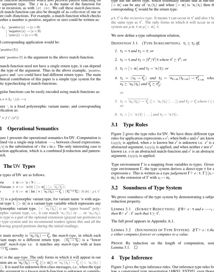
Figure 1 presents the operational semantics forDV. Computation is defined via a single-step relation−→1between closed expressions. e[v/x]is the substitution ofvforxine. The only interesting case is function application, which is a combinedβ-reduction and pattern-match.
3
The
DV
Types
The types ofDVare as follows. TyVar 3α::= 0a|0b|. . .
TypVariant3ν::= ‘n(τ)|[>α]|[<‘nk(τk) ]
Typ 3τ::= α|Int|ν|‘nk(τk)→τ0k| hνk→τki |τ(ν)|µτ.τ0 ‘n(τ)is a polymorphic variant type, for variant name ‘n with argu-ment typeτ. [>α]is a variant-type variable which represents any polymorphic variant type. [< ‘nk(τk) ]is an “upper bound”
poly-morphic variant type, i.e., it can match ‘n1(τ1)or. . .or ‘nk(τk).
This type is a part of the optional extension (grayed out portions) to our type system and we recommend readers ignore this and all the following grayed portions during the initial readings.
Our main novelty is ‘nk(τk)→τ0k, the match-type, in which each variant maps to a different return type. hνk→τki is a “lower bound” match-type i.e. it matches any match-type with at least
νk→τkcases.
τ(ν)is the app-type. The only forms in which it will appear in our system are as ‘nk(τk)→τ0k([>α])or ‘nk(τk)→τ0k([<‘ni(τi)| . . .]). It is used for unknown first-class messages, i.e., when the type of the argument to a known match-function is unknown at compile-time, and the return type is also unknown and depends upon the
value assigned to the argument at run-time. In such cases, the return type has the above type, which essentially means that at run-time
[> α]can be any of ‘ni(τi)and when [> α]is ‘ni(τi)then the correspondingτ0iwould be the return type.
µτ.τ0is the recursive-type. It meansτcan occur inτ0and alsoτhas
the same type asτ0. The only forms in which it will occur in our
system are µα.τor µ[>α].τ.
We now define a type subsumption relation,
DEFINITION3.1 (TYPESUBSUMPTION). τ1τ2iff, 1. τ1=τandτ2=τ; or 2. τ1=τandτ2= [τ00/τ0]τwhereτ0τ00; or 3. τ1= [>α]andτ2=‘n(τ); or 4. τ1 = hνk→τ0ki and τ2 = ‘nk+m(τk+m)→τ00k+m where νk‘nk(τk)andτ0kτ00k; or
5. τ1=‘nk(τk)→τ0k([<‘ni(τi)|. . .])andτ2=τ0iwhere i≤k;
or
6. τ1= [<‘n(τ)|. . .]andτ2=‘n(τ).
3.1
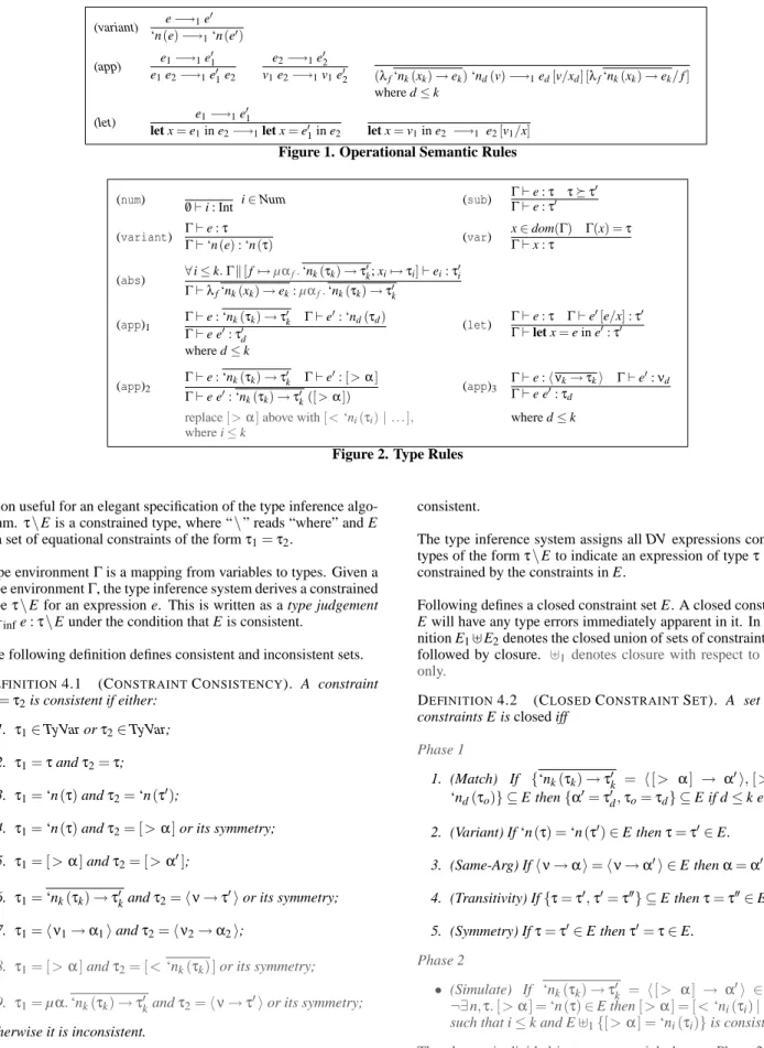
Type Rules
Figure 2 gives the type rules forDV. We have three different types rules for application expressions e e0; when both e and e0are known (app)1is applied, when e is known but e0is unknown i.e. e0is an abstracted argument, (app)2is applied, and when neither e nor e0is known i.e. e is an abstracted match-function and e0is an abstracted argument, (app)3is applied.
Type environmentΓis a mapping from variables to types. Given a type environmentΓ, the type system derives a direct-typeτfor an expression e. This is written as a type judgementΓ`e :τ.Γk[xi7→
αi]is the extension ofΓwith xi7→αi.
3.2
Soundness of Type System
We prove soundness of the type system by demonstrating a subject reduction property.
LEMMA3.1 (SUBJECTREDUCTION). If/0`e :τand e−→1e0 then/0`e0:τ0such thatττ0.
The full proof appears in Appendix A.1.
LEMMA3.2 (SOUNDNESS OFTYPESYSTEM). IfΓ`e :τthen e either computes forever or computes to a value.
PROOF. By induction on the length of computation, using Lemma 3.1.
4
Type Inference
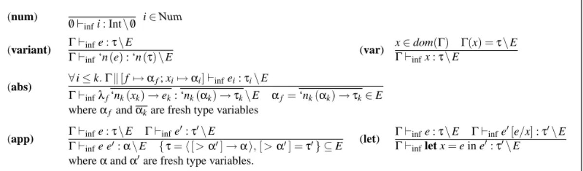
Figure 3 gives the type inference rules. Our inference type rules fol-low a constrained type presentation [AW93, EST95], even though our type theory does not include subtyping. We found this
formu-(variant) e−→1e 0 ‘n(e)−→1‘n(e0) (app) e1−→1e 0 1 e1e2−→1e01e2 e2−→1e02 v1e2−→1v1e02 (λf‘nk(xk)→ek)‘nd(v)−→1ed[v/xd] [λf‘nk(xk)→ek/f] where d≤k (let) e1−→1e 0 1
let x=e1in e2−→1let x=e01in e2 let x=v1in e2 −→1 e2[v1/x] Figure 1. Operational Semantic Rules
(num) /0
`i : Int i∈Num (sub)
Γ`e :τ ττ0 Γ`e :τ0 (variant) Γ`e :τ Γ`‘n(e): ‘n(τ) (var) x∈dom(Γ) Γ(x) =τ Γ`x :τ (abs) ∀i≤k.Γk[f7→µαf.‘nk(τk)→τ 0 k; xi7→τi]`ei:τ0i Γ`λf‘nk(xk)→ek:µαf.‘nk(τk)→τ0k (app)1 Γ `e : ‘nk(τk)→τ0k Γ`e 0: ‘n d(τd) Γ`e e0:τ0d (let) Γ`e :τ Γ`e 0[e/x]:τ0 Γ`let x=e in e0:τ0 where d≤k (app)2 Γ `e : ‘nk(τk)→τk0 Γ`e0:[>α] Γ`e e0: ‘n k(τk)→τ0k([>α]) (app)3 Γ `e :hνk→τki Γ`e0:νd Γ`e e0:τd
replace[>α]above with[<‘ni(τi)|. . .], where d≤k where i≤k
Figure 2. Type Rules
lation useful for an elegant specification of the type inference algo-rithm.τ\E is a constrained type, where “\” reads “where” and E is a set of equational constraints of the formτ1=τ2.
Type environmentΓis a mapping from variables to types. Given a type environmentΓ, the type inference system derives a constrained typeτ\E for an expression e. This is written as a type judgement Γ`infe :τ\E under the condition that E is consistent.
The following definition defines consistent and inconsistent sets. DEFINITION4.1 (CONSTRAINTCONSISTENCY). A constraint
τ1=τ2is consistent if either: 1. τ1∈TyVarorτ2∈TyVar; 2. τ1=τandτ2=τ; 3. τ1=‘n(τ)andτ2=‘n(τ0);
4. τ1=‘n(τ)andτ2= [>α]or its symmetry; 5. τ1= [>α]andτ2= [>α0];
6. τ1=‘nk(τk)→τ0kandτ2=hν→τ0ior its symmetry; 7. τ1=hν1→α1iandτ2=hν2→α2i;
8. τ1= [>α]andτ2= [<‘nk(τk) ]or its symmetry;
9. τ1=µα.‘nk(τk)→τ0kandτ2=hν→τ0ior its symmetry; Otherwise it is inconsistent.
A constraint set E is consistent if all the constraints in the set are
consistent.
The type inference system assigns allDVexpressions constrained types of the formτ\E to indicate an expression of typeτwhich is constrained by the constraints in E.
Following defines a closed constraint set E. A closed constraint set E will have any type errors immediately apparent in it. In the defi-nition E1]E2denotes the closed union of sets of constraints: union followed by closure. ]1 denotes closure with respect to Phase 1 only.
DEFINITION4.2 (CLOSEDCONSTRAINTSET). A set of type constraints E is closed iff
Phase 1
1. (Match) If {‘nk(τk)→τ0k = h[> α] → α0i,[> α] = ‘nd(τo)} ⊆E then{α0=τ0d,τo=τd} ⊆E if d≤k else fail.
2. (Variant) If ‘n(τ) =‘n(τ0)∈E thenτ=τ0∈E. 3. (Same-Arg) Ifhν→αi=hν→α0i ∈E thenα=α0∈E. 4. (Transitivity) If{τ=τ0,τ0=τ00} ⊆E thenτ=τ00∈E. 5. (Symmetry) Ifτ=τ0∈E thenτ0=τ∈E. Phase 2 • (Simulate) If ‘nk(τk)→τ0k = h[> α] → α0i ∈ E and ¬∃n,τ.[>α] =‘n(τ)∈E then[>α] = [<‘ni(τi)|. . .]∈E,
such that i≤k and E]1{[>α] =‘ni(τi)}is consistent. The closure is divided in two sequential phases. Phase 2 is com-puted only after Phase 1 completes.
(num) /0`infi : Int\/0 i∈Num (variant) Γ`infe :τ\E Γ`inf‘n(e): ‘n(τ)\E (var) x∈dom(Γ) Γ(x) =τ\E Γ`infx :τ\E (abs) ∀i≤k.Γk[f7→αf; xi7→αi]`infei:τi\E Γ`infλf‘nk(xk)→ek: ‘nk(αk)→τk\E αf=‘nk(αk)→τk∈E whereαf andαkare fresh type variables
(app) Γ`infe :τ\E Γ`infe 0:τ0\E
Γ`infe e0:α\E {τ=h[>α0]→αi,[>α0] =τ0} ⊆E (let)
Γ`infe :τ\E Γ`infe0[e/x]:τ0\E Γ`inflet x=e in e0:τ0\E whereαandα0are fresh type variables.
Figure 3. Type Inference Rules
The (Match) rule is the crux of our type inference system. It en-ables match-functions to choose the return type corresponding to the argument type. The closure rule for normal functions is “if
τ1→τ01=τ→τ0∈E then{τ=τ1,τ01=τ0} ⊆E”. (Match) is the generalization of this rule to match-functions. When the argu-ment type to the match-function is known, i.e. it is ‘nd(τo), then
(Match) simply selects the matching sub-function and applies the above regular function closure rule. Unknown arguments introduce no immediate type errors and so are not analyzed. If the variant is not in the match-type, there is no closure of E: closure fails. (Variant) ensures that if two variants are equal they have the same argument type.
(Same-Arg) ensures that identical variants applied to the same match-function have identical component types.
(Simulate) adds precision to the type of an unknown argument
ap-plied to a known match-function. So if ‘nk(τk)→τ0k=h[>α]→
α0i ∈E but¬∃n,τ.[>α] =‘n(τ)∈E after Phase 1, then[>α]
doesn’t have a known concrete type. However, the above constraint
does imply that[>α]could have been ‘n1(τ1)or ‘n2(τ2)or . . . or
‘nk(τk), and it would still have been consistent; anything else would
have made it inconsistent. So to find all the valid ‘ni(τi)’s we add
[>α] =‘ni(τi)to E for all i≤k separately and compute the
clo-sure with respect to Phase 1. If the resulting closed set is consistent
we know that ‘ni(τi)is a valid type for[>α]. At the end of all the
simulations we add[>α] = [<‘ni(τi)|. . .]to E where ‘ni(τi)is a valid type for[>α].
The closure is trivially seen to be computable in O(n3)time, as-suming Kn, where n=|E|and K=max(k)∀k.‘nk(τk)→τ0k=
hτ→α0i ∈E. In the rare case where K≈n, the time complexity would be O(n3K). The factor K is introduced due to (Match) hav-ing to search through at most each of the K sub-functions to find a match (or an absence thereof).
We now define the type inference algorithm.
ALGORITHM4.1 (TYPE INFERENCE). Given an expression e its typeτ\E (or type-error) can be inferred as follows:
1. Produce the unique proof tree /0`e :τ\E via the type infer-ence rules in Figure 3.
2. Compute E+=closure(E).
3. If E+is consistent thenτ\E+is the inferred type for e, else there is a type-error in e.
By inspection of the type inference rules in Figure 3, it is easy to see this process is deterministic, based on the structure of e, modulo the choice of fresh type variables.
We don’t prove the soundness of the type inference algorithm. Rather we give a Simpfication Algorithm 4.2, which simplifies the inferred constrained types to direct-types as per the type rules in Figure 2 which we have already proven sound, and prove the sound-ness of this simplification algorithm. However, it would not be very difficult to verify that the soundness of the type inference algorithm as well.
4.1
Equational Simplification
Now we present an algorithm for reducing a constrained typeτ\E
to an unconstrained typeτs which contains all the type
informa-tion ofτ\E, and prove its soundness. This means direct types
containing the complete type information, without hard-to-digest type equations, can be presented to programmers. This improves on [Gar98] which is a lossy method.
We now give the algorithm for simplification. In the following al-gorithm we handle symmetry implicitly.
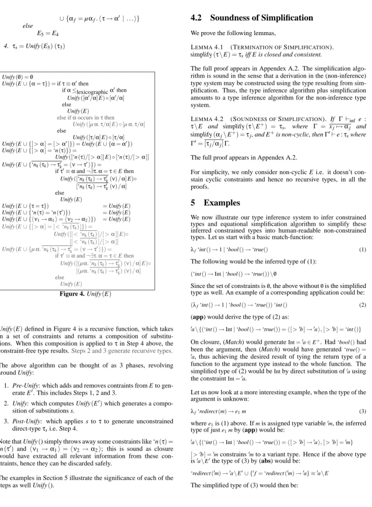
ALGORITHM4.2 (SIMPLIFICATION). A constrained typeτ\E can be reduced toτsby the following steps:
1. For all constraints of the formα=hν→τ0i ∈E E1=E− {α=hν1→τ10i, . . . ,α=hνk→τ0ki}
∪ {α=hνk→τ0ki}
2. For all constraint sets of the form{αf =‘nk(τk)→τ0k,[>
α] =τ,αf=h[>α]→α0|. . .i} ⊆E1, E2a=E1− {αf=‘nk(τk)→τ0k} τ2\E2= [µαf.‘nk(τk)→τ0k/‘nk(τk)→τ0k] (τ\E2a) ifτoccurs in ‘nk(τk)→τ0kthen: τ3\E3= [αf([>α])/α0] (τ2\E2) else τ3\E3=τ2\E2 E4=E3− {αf=h[>α]→α0|. . .i}
3. For all constraint sets of the form {[> α] =τ,αf =h[> α]→α0|. . .i} ⊆E
4,
ifαfoccurs inτthen:
∪ {αf =µαf.hτ→α0|. . .i} else E5=E4 4. τs=Unify(E5) (τ3) Unify(/0) =/0 Unify(E∪ {α=τ}) =ifτ≡α0then ifα≤lexicographicα0then Unify([α0/α]E)◦[α0/α] else Unify(E)
else ifαoccurs inτthen
Unify([µα.τ/α]E)◦[µα.τ/α] else Unify([τ/α]E)◦[τ/α] Unify(E∪ {[>α] = [>α0]}) =Unify(E∪ {α=α0}) Unify(E∪ {[>α] =‘n(τ)}) = Unify([‘n(τ)/[>α]]E)◦[‘n(τ)/[>α]] Unify(E∪ {‘nk(τk)→τ0k=hν→τ 0i}) = ifτ0≡αand¬∃τ.α=τ∈E then Unify([‘nk(τk)→τ0k(ν)/α]E)◦ [‘nk(τk)→τ0k(ν)/α] else Unify(E) Unify(E∪ {τ=τ}) =Unify(E) Unify(E∪ {‘n(τ) =‘n(τ0)}) =Unify(E) Unify(E∪ {hν1→α1i=hν2→α2i}) =Unify(E) Unify(E∪ {[>α] = [<‘nk(τk) ]}) = Unify([[<‘nk(τk) ]/[>α]]E)◦ [[<‘nk(τk) ]/[>α]] Unify(E∪ {µα.‘nk(τk)→τ0k=hν→τ 0i}) = ifτ0≡αand¬∃τ.α=τ∈E then Unify([(µα.‘nk(τk)→τ0k) (ν)/α]E)◦ [(µα.‘nk(τk)→τ0k) (ν)/α] else Unify(E) Figure 4. Unify(E)
Unify(E)defined in Figure 4 is a recursive function, which takes in a set of constraints and returns a composition of substitu-tions. When this composition is applied toτin Step 4 above, the constraint-free type results.Steps 2 and 3 generate recursive types.
The above algorithm can be thought of as 3 phases, revolving around Unify:
1. Pre-Unify: which adds and removes contraints from E to gen-erate E0. This includes Steps 1, 2 and 3.
2. Unify: which computes Unify(E0)which generates a compo-sition of substitutions s.
3. Post-Unify: which applies s to τto generate unconstrained direct-typeτsi.e. Step 4.
Note that Unify() simply throws away some constraints like ‘n(τ) =
‘n(τ0) and hν1→α1i=hν2 →α2i; this is sound as closure would have extracted all relevant information from these con-straints, hence they can be discarded safely.
The examples in Section 5 illustrate the significance of each of the steps as well Unify().
4.2
Soundness of Simplification
We prove the following lemmas,
LEMMA4.1 (TERMINATION OFSIMPLIFICATION).
simplify(τ\E) =τsiff E is closed and consistent.
The full proof appears in Appendex A.2. The simplification algo-rithm is sound in the sense that a derivation in the (non-inference) type system may be constructed using the type resulting from sim-plification. Thus, the type inference algorithm plus simplification amounts to a type inference algorithm for the non-inference type system.
LEMMA4.2 (SOUNDNESS OFSIMPLIFCATION). If Γ `inf e : τ\E and simplify(τ\E+) = τs, where Γ = xj7→αj and
simplify(αj\E+) =τj, and E+is non-cyclic, thenΓ0`e :τswhere
Γ0= [τ j/αj]Γ.
The full proof appears in Appendex A.2.
For simplicity, we only consider non-cyclic E i.e. it doesn’t con-stain cyclic constraints and hence no recursive types, in all the proofs.
5
Examples
We now illustrate our type inference system to infer constrained types and equational simplification algorithm to simplify these inferred constrained types into human-readable non-constrained types. Let us start with a basic match-function:
λf‘int()→1|‘bool()→‘true() (1)
The following would be the inferred type of (1):
(‘int()→Int|‘bool()→‘true())\/0
Since the set of constraints is/0, the above without/0is the simplified type as well. An example of a corresponding application could be:
(λf‘int()→1|‘bool()→‘true())‘int() (2) (app) would derive the type of (2) as:
0a\ {(‘int()→Int|‘bool()→‘true()) =h[>0b]→0ai,[>0b] =‘int()}
On closure, (Match) would generateInt=0a∈E+. Had‘bool()had
been the argument, then (Match) would have generated‘true() = 0a, thus achieving the desired result of tying the return type of a
function to the argument type instead to the whole function. The simplified type of (2) would beIntby direct substitution of0ausing
the constraintInt=0a.
Let us now look at a more interesting example, when the type of the argument is unknown:
λf‘redirect(m)→e1m (3)
wheree1is (1) above. Ifmis assigned type variable0m, the inferred type of juste1mby (app) would be:
0a\ {(‘int()→Int|‘bool()→‘true()) =h[>0b]→0ai,[>0b] =0m} [>0b] =0mconstrains0mto a variant type. Hence if the above type
is0a\E0the type of (3) by (abs) would be:
‘redirect(0m)→0a\E0∪ {0f=‘redirect(0m)→0a} ≡0a\E
‘redirect([>0b])→(‘int()→Int|‘bool()→‘true()) [>0b]
or
‘redirect([<‘int()|‘bool() ])→
(‘int()→Int|‘bool()→‘true()) [<‘int()|‘bool() ] mainly due toUnify()on‘int()→Int|‘bool()→‘true() =h[>0b]→0ai and Phase 2 of closure. As is clearly evident this simplified type is
more precise but verbose and hence less-readable as well.
Now consider the following application with first-class message passing where‘int()is the first-class message:
(λf‘redirect(m)→e1m) (‘redirect(‘int())) (4) (app) would infer its type as:
0b\E∪ {‘redirect(0m)→0a=h[>0c]→0bi,[>0c] =‘redirect(‘int())}
The simplified type of (4) would beInt. Let us go through the steps. (Match) closure on the above constraint generates:
{0a=0b,‘int() =0m}
Next,‘int() =0mwith[>0b] =0mon (Transitivity) gives[>0b] =0m
and{(‘int()→Int|‘bool()→‘true()) =h[>0b]→0ai,[>0b] =‘int()}
on (Match) generates:
mathrmInt=0b
Unify() withInt=0bgenerates a substitution[Int/0b]and hence the
simplified type isInt.
Lets now consider the case when the match-function is unknown:
λf‘dummy(o)→o(‘zero()) (5)
(abs) with (app) will infer the following constrained type:
‘dummy(0o)→0b\ {0o=h[>0c]→0bi,[>0c] =‘zero()}
The simplified type would be:
‘dummy(h‘zero()→0bi)→0b
by Step 1 of Algorithm 4.2 and substitutions by Unify(). Now consider a minor variant of (5):
λf‘dummy(o)→o(‘m()); o(‘n()) (6)
The simplified type of (6) mainly by Step 1 of Algorithm 4.2 would be:
‘dummy(h‘m()→0a|‘n()→0bi)→0b
Let us look at the case when both the match-function and the argu-ment is unknown:
λf‘dummy(o)→λf‘redirect(m)→o m (7) (abs) and (app) would infer the type of (7) as:
‘dummy(0o)→‘redirect(0m)→0a\ {0o=h[>0b]→0ai,[>0b] =0m}
and the simplified type would be:
‘dummy(h[>0b]→0ai)→‘redirect([>0b])→0a
Now lets consider the most complicated examplewhich shows the
real usefulness of (Simulate) closure rule:
λf‘redirect(m)→(λf‘a(x)→x>0|‘b(x)→x+1)m;
(λf ‘b(x)→x+0|‘c(x)→x==1)m (8)
It can be deduced by inspection thatmcould only be substituted
‘b at run-time since it is the only variant name present in both match-functions and hence the return type ofλfredirectcould only beIntand neverBool.
Our system (without Closure Phase 2) will, however, generate only the following constraints even after closure:
{(‘a(x)→Bool|‘b(x)→Int) =h[>0m
1]→0ei,[>0m1] =0m (‘b(x)→Int|‘c(x)→Bool) =h[>0m2]→0fi,[>0m2] =0m}
There is no constraint on return types0eand0f nor any constraint
of the form0m=Int. This constraint set is still consistent since the
messagemin the program is not sent and hence the above code is essentially dead. The simplified type of (8), anologous to that of (3), would be:
‘redirect([>0m2])→(‘b()→Int|‘c()→Bool) [>0m2] Ifmwere sent in the future as say‘a(5), then the constraints {(‘b(x)→Bool|‘c(x)→Int) =h[>0m2]→0fi,[>0m2] =‘a(Int)} would be generated and (Match) would fail. Thus the program would not typecheck.
Had (Simulate) been computed, it would have generated [>0m1] = [<‘b() ],[>0m2] = [<‘b() ]
resulting in the simplified type of (8) to be:
‘redirect([<‘b() ])→(‘b()→Int|‘c()→Bool) [<‘b() ]
which clearly implies thatInt is the only possible return type for
‘redirect.
Now lets take a look at expressions which result in cyclic types
i.e.µα.τ. Neither type derivation nor closure generate cyclic types;
they are only generated duringsimplify(),
λf‘this()→f (9)
The simplified type would be:
µ0f.‘this()→0f
maily due to Step 2 of Algorithm 4.2. Consider a similar example:
λf‘this(x)→f x (10)
The simplified type would be:
µ0f.‘this([>0a])→(0f) [>0a]
and with (Simulate)
µ0f.‘this(µ[>0a].[<‘this([>0a]) ])→ 0f(µ[>0a].[<‘this([>0a]) ] )
maily due to Step 2 of Algorithm 4.2 andUnifyon cyclic constraint
0m= [<‘this(0m) ]such that0m= [>0a]is in the generated set of
con-straints.
Lets consider an example of self-application:
λ‘dummy(x)→x(‘self(x)) (11)
The simplified type will be:
maily due to Step 3 of Algorithm 4.2.
6
Encoding Objects and Other Features
We now show how a collection of simple macros allow object-based programs to be faithfully encoded intoDV.
The basic idea is to encode classes and objects as match-functions and messages as polymorphic variants, thus reducing message-sending to simple function application. There is nothing unusual in the translation itself, the main feature is the expressiveness of its typing: match types allow arbitrary objects to typecheck encoding messages as variants.
DEFINITION 6.1. The object syntax is defined by the following translation.
(class) Jclass(λthis ‘nk(xk)→ek)K=λthis →λthis ‘nk(xk)→JekK
(new) Jnew eK=JeK()
(send) Je1←e2K=Je1K Je2K
(message) J‘n(e)K=‘n(JeK)
Since match-functions are recursive, we get recursive objects with this for self-reference within the object. We now illus-trate this encoding with ftpProxyexample from the introduction.
Jlet ftp=new(class(λf‘get()→1))in
let ftpProxy=
new(class(λf‘send(m)→(ftp←m)))in ftpProxy←‘send(‘get())K ⇓(translation to DV) let ftp= (λf →λf‘get()→1) ()in let ftpProxy= (λf →λf‘send(m)→(ftp m)) ()in ftpProxy ‘send(‘get())
It creates newftpandftpProxyobjects withftpProxydelegating mes-sages toftp. For simplicity,ftpreturns an integer in response to the
‘getrequest.
The simplified type offtpProxyproduced by our system would be:
‘send([>0m])→(‘get()→Int) [>0m] and with (Simulate):
‘send([<‘get() ])→(‘get()→Int) ([<‘get() ])
which is similar to example (3) in Section 5. We do not deal with inheritance here, but the various standard approaches should apply. We show that records and if-then-else can also be encoded with variants and match-types alone, thus defining a very expressive lan-guage.
6.1
Encoding Records
In Section 1.1 we discussed the duality of variants and records. We showed how the ML type system allows only records with all ele-ments of the same type to be encoded in terms of variants. We now show how match-functions can fully and faithfuly encode records. This should not be surprising given the above encoding of objects. A match-function is essentially a sophisticated form of the ML match statement. Hence, record encoding of a match-function would be identical to that ofmatchgiven in Section 1.1. The key
observation is that, since every case of the match can return a dif-ferent type, it allows records with difdif-ferently-typed fields to be en-coded. For example, the record{l1=5,l2=‘wow(3)}is encoded as λf‘l1(x)→5|‘l2(x)→‘wow(3)and has type(‘l1(0a)→Int|‘l2(0b)→ ‘wow(Int)).
6.2
Encoding if-then-else
if-then-else statements can be easily encoded via match-functions using polymorphic variants ‘true() and ‘false() to correspond to boolean valuestrueandfalserespectively. This encoding has the added advantage that the two “branches” can have different return types. if-then-else is then encoded as
Jif e then e1else e2K= (λf‘true()→e1|‘false()→e2)e
7
Related Work
Previous papers containing static type systems for first class mes-sages include those by Wakita [Wak93], Nishimura [Nis98], M¨uller & Nishimura [MN00], and Pottier [Pot00]. The main advantage of our system is it is significantly simpler. No existing program-ming language implementation efforts have included typed first-class messages, this is an implicit indication of a need for a more simple type system that captures their spirit.
Wakita [Wak93] presents an inter-object communication frame-work based on RPC-like message passing. He does not present a type system for his language so a comparision with his system is not possible.
Nishimura [Nis98] develops a second order polymorphic type sys-tem for first-class messages (referring to them as dynamic messages in the paper), where type information is expressed by kindings of the form t :: k, where t is a type variable indexing the type informa-tion of the object or message and k is a kind representing the type information. It has no type directly representing the type struc-ture of objects and messages. This system is very complicated and M¨uller and Nishimura in [MN00] (same second author) attempt to present a simpler system.
M¨uller et al [MN00] present a monomorphic type inference system based on OF (objects and features) constraints. They extend tradi-tional systems of feature constraints by a selection constraint xhyiz intended to model the behavior of a generic message-send opera-tion. This does simplify things a little, but, is arguably still not simple enough to be implemented in a programming language. Bugliesi and Crafa [BC99] also attempt to simplify Nishimura’s original work [Nis98]. However, they choose a higher-order type system, and abandon type inference.
Pottier [Pot00] like us does not define a type system oriented solely around first-class messages; it is a very general type system that happens to be powerful enough to also faithfully type first-class messages. His approach is in some ways similar to ours in that conditional types are used. His system is very expressive, but is also very complex and is thus more suited to program analysis than the production of human-readable types.
8
Implementation
We have implemented an interpreter forDVin OCaml. It has an OCaml-style top-loop, in which the user can feed aDVexpression.
The interpreter will typecheck it, compute its simplified human-readable type, evaluate it to a value and then display both the value and the type.
The core of the interpreter, which includes the Type Inference (4.1) and Simplification (4.2) Algorithms, is only a few hundred lines of code. This further validates our assertion about the simplicity of the
DVtype system.
The source code along with documentation and examples can be found athttp://www.cs.jhu.edu/˜pari/match-functions/. Acknowledgements
We would like to thanks the anonymous reviewers for their com-ments on improving the paper.
9
References
[AW93] Alexander Aiken and Edward L. Wimmers. Type in-clusion constraints and type inference. In Functional Programming Languages and Computer Architecture, pages 31–41, 1993.
[BC99] Michele Bugliesi and Silvia Crafa. Object calculi with dynamic messages. In FOOL’6, 1999.
[EST95] Jonathan Eifrig, Scott Smith, and Valery Trifonov. Type inference for recursively contrained types and its application to oop. In Electronic Notes in Theoretical Computer Science, volume 1, 1995.
[Gar98] Jacques Garrigue. Programming with polymorphic variants. In ML Workshop, 1998.
[Gar00] Jacques Garrigue. Code reuse through polymorphic variants. In Workshop on Foundations of Software En-gineering, 2000.
[GR89] Adele Goldberg and David Robson. Smalltalk-80 The Language. Addison-Wesley, 1989.
[LDG+02] Xavier Leroy, Damien Doligez, Jacques Garrigue, Di-dier R´emy, and J´erˆome Vouillon. The Objective Caml system release 3.06, Documentation and user’s manual. INRIA, http://caml.inria.fr/ocaml/htmlman/, 2002.
[MN00] Martin M¨uller and Susumu Nishimura. Type inference for first-class messages with feature constraints. Inter-national Journal of Foundations of Computer Science, 11(1):29–63, 2000.
[Nis98] Susumu Nishimura. Static typing for dynamic mes-sages. In POPL’98: 25th Annual ACM SIGPLAN-SIGACT Symposium on Principles of Programming Languages, 1998.
[Oho95] Atsushi Ohori. A polymorphic record calculus and its compilation. ACM Transactions on Programming Lan-guages and Systems, 17(6):844–895, November 1995. [Pot00] Franc¸ois Pottier. A versatile constraint-based type
in-ference system. Nordic Journal of Computing, 7:312– 347, 2000.
[PW91] Lewis J. Pinson and Richard S. Wiener. Objective-C: Object Oriented Programming Techniques. Addison-Wesley, 1991.
[R´89] Didier R´emy. Type checking records and variants in a
natural extension of ML. In POPL, pages 77–88, 1989. [Wak93] Ken Wakita. First class messages as first class continu-ations. In Object Technologies for Advanced Software, First JSSST International Symposium, 1993.
A
Proofs
A.1
Soundness of the Type System
We prove soundness of the type system by demonstrating a subject reduction property.
LEMMAA.1.1 (SUBSTITUTION). IfΓk[x7→τx]`e :τandΓ`e0:τ0xsuch thatτxτ0x, thenΓ`e[e0/x]:τ0such thatττ0.
PROOF. Follows induction on the structure of e. For simplicity we ignore the (sub) case as well as recursive match-functions. 1. (num) e≡i. Proof is trivial.
2. (var) e≡x and x∈dom(Γ). By (var),Γ`x :τwhereΓ(x) =τ.
By induction hypothesis, letΓ(x[e0/x]) =τ0whereττ0. Hence, by (var),Γ`x[e0/x]:τ0.
3. (variant) e≡‘n(ev)
By (variant), letΓ`‘n(ev): ‘n(τv)whereΓ`ev:τv. Also let x7→τx∈Γ.
By induction hypothesis, letΓ0`ev[e0/x]:τ0vandΓ0`e0:τx0, whereΓ0=Γ− {x7→τx}such thatτxτ0xandτvτ0v.
Now, ‘n(ev) [e0/x] =‘n(ev[e0/x]). Hence, by (variant),Γ0`‘n(ev[e0/x]): ‘n(τ0v). Also, by Case 6 of Definition 3.1, ‘n(τv)‘n(τ0v). 4. (abs) e≡‘nk(xk)→ek
By (abs),Γ`‘nk(xk)→ek: ‘nk(τk)→τ0kwhere∀i≤k.Γk[xi7→τi]`ei:τ 0
i. Also let x7→τx∈Γand, without loss of generality,
x∈ {x/ i}.
By induction hypothesis, let∀i≤k.Γ0k[xi7→τi]`ei[e0/x]:τ00i, whereΓ`e0:τ0xandΓ0=Γ− {x7→τx}such thatτxτ0xandτ0kτ00k. Now, (‘nk(xk)→ek)[e0/x] =‘nk(xk)→(ek[e0/x]). Thus, by (abs),Γ0`‘nk(xk)→(ek[e0/x]): ‘nk(τk)→τ00k. Also, by Case 2 of Definition 3.1, ‘nk(τk)→τ0k‘nk(τk)→τ00k.
5. (app) e≡eoev. There are 3 different cases:
(a) (app)1. By (app)1,Γ`eoev:τ0dwhereΓ`eo: ‘nk(τk)→τ0k,Γ`ev: ‘nd(τd)for d≤k. Also, let x7→τx∈Γ.
By induction hypothesis and Case 2 of Definition 3.1, letΓ0`eo[e0/x]: ‘nk(τ00k)→τ000kandΓ0`ev[e0/x]: ‘nd(τ00d)whereΓ`e0:τ0x andΓ0=Γ− {x7→τx}such thatτxτx0,τkτ00kandτ0kτ000k.
Now,(eoev) [e0/x] = (eo[e0/x]) (ev[e0/x]). Thus, by (app)1,Γ0`(eo[e0/x]) (ev[e0/x]):τ000dand by hypothesis we knowτ0dτ000d.
(b) (app)2. By (app)2,Γ`eoev: ‘nk(τk)→τ0k([< ‘ni(τi)|. . .])whereΓ`eo: ‘nk(τk)→τ0k,Γ`ev:[<‘ni(τi)|. . .]for i≤k. Also, let x7→τx∈ΓandΓ0=Γ− {x7→τx}. Assume,Γ`e0:τ0xsuch thatτxτ0x. Also,(eoev) [e0/x] = (eo[e0/x]) (ev[e0/x]). Now there two possible choices for the induction hypothesis :
i. By induction hypothesis and Case 2 of Definition 3.1, letΓ0`eo[e0/x]: ‘nk(τ00k)→τ000kandΓ0`ev[e0/x]:[<‘ni(τ00i)|. . .]
such thatτkτ00
kandτ0kτ000k.
Thus, by (app)2, Γ0 ` (eo[e0/x]) (ev[e0/x]) : ‘nk(τ00k)→τ000k ([< ‘ni(τ00i) | . . .]) and by Case 2 of Definition 3.1, ‘nk(τk)→τ0k([<‘ni(τi)|. . .])‘nk(τ00k)→τ000k([<‘ni(τ00i)|. . .]).
ii. By induction hypothesis and Cases 2 and 6 of Definition 3.1, letΓ0`eo[e0/x]: ‘nk(τ00k)→τ000kandΓ0`ev[e0/x]: ‘ni(τ00i)for
some i≤k such thatτkτ00
Thus, by (app)2,Γ0`(eo[e0/x]) (ev[e0/x]):τ000iand by Cases 2 and 5 of Definition 3.1, ‘nk(τk)→τk0 ([<‘ni(τi)|. . .]) ‘nk(τ00k)→τ000k([<‘ni(τ00i)|. . .])τ000i.
(c) (app)3. By (app)3,Γ`eoev:τdwhereΓ`eo:hνk→τki,Γ`ev:νdfor d≤k. Also, let x7→τx∈ΓandΓ0=Γ− {x7→τx}. Assume,Γ`e0:τ0xsuch thatτxτ0x. Also,(eoev) [e0/x] = (eo[e0/x]) (ev[e0/x]).
Now there two possible choices for the induction hypothesis :
i. By induction hypothesis and Case 2 of Definition 3.1, letΓ0`eo[e0/x]:hν0k→τ0kiandΓ0`ev[e0/x]:ν0dsuch thatνkν0k andτkτ0k.
Now,(eo ev) [e0/x] = (eo[e0/x]) (ev[e0/x]). Thus, by (app)3,Γ0`(eo[e0/x]) (ev[e0/x]):τ0d and we know by hypothesis
τdτ0d.
ii. By induction hypothesis, let Γ0`eo[e0/x]: ‘nk+l(τ0k+l)→τ00k+l and Γ0`ev[e0/x]: ‘nd(τ0d) such that νk‘nk(τ0k) and
τkτ00k.
Thus, by (app)3,Γ0`(eo[e0/x]) (ev[e0/x]):τ00dand we know by hypothesisτdτ00d. 6. (let) e≡let y=e1in e2.
By (let), letΓ`e :τ2whereΓ`e1:τ1andΓ`e2[e1/y]:τ2. Also, let x7→τx∈Γ. Without loss of generality, we assume x6=y. By induction hypothesis, letΓ0`e1[e0/x]:τ01,Γ0`e2[e1/y] [e0/x]:τ20 andΓ`e0:τ0x, whereΓ0=Γ− {x7→τx}such thatτxτ0x,τ1τ01 andτ2τ02.
Now, x6=y implies(let y=e1in e2) [e0/x] =let y=e1[e0/x]in e2[e0/x]. Similarly, e2[e1/y] [e0/x] =e2[e0/x] [e1/y]. Hence by (let), Γ0`e[e0/x]:τ0
2.
LEMMAA.1.2 (SUBJECTREDUCTION). If/0`e :τand e−→1e0then/0`e0:τ0such thatττ0.
PROOF. Follows by strong induction on the depth of the type derivation tree, i.e., the induction hypothesis applies to all trees of depth n−1 or less, where n is the depth of the proof tree of/0`e :τ. Hence, following are all the possible rules that can be applied as the last step of the type derivation of/0`e :τ. (Note that (app)2and (app)3, will never be applied as the last step, since the argument in (app)2and both the applicand and the argument in (app)3are program variables, and hence the application expression is not closed. By the same argument (var) will also never be the last step. These cases are handled in the Substitution Lemma.)
1. (num). Proof is trivial. 2. (variant).
Hence, e≡‘n(ed)and let the last step of the type derivation be/0`‘n(ed): ‘n(τd)and/0`ed:τdthe penultimate one. By (variant), ‘n(ed)−→1‘n(e0d)where ed−→1e0d.
By induction hypothesis, let/0`e0d:τ0dsuch thatτdτ0d. Hence by (variant),/0`‘n(ed0): ‘n(τ0d). We know by Case 6 of Definition 3.1, ‘n(τd)‘n(τ0d).
3. (abs)
Hence, e≡‘nk(αk)→ek. The proof in this case trivial, since a ‘nk(αk)→ek∈Val, hence it evaluates to itself. 4. (app)1
Hence, e≡eoev. The cases when eoand evare not both values are analogous to Case 2. Suppose now that both eo,ev∈Valthen
e≡(λf‘nk(xk)→e0k)‘n(v).
Hence by (app)1, let the the last step of the type derivation be/0`e :τ0dfor d≤k and,/0`λf‘nk(xk)→e0k: ‘nk(τk)→τk0,∀i≤k./0k[f7→ ‘nk(τk)→τ0k; xi7→τi]`ei:τ0iand /0`‘n(v): ‘nd(τd)be the penultimate ones, where n≡nd; while be/0`v :τdthe second to last.
By (app), let e−→1ed[v/xd] [λf‘nk(xk)→e0k/f]≡e0. Now by Lemma A.1.1,/0`e0:τ00dsuch thatτ0dτ00d. 5. (let)
Hence, e≡let x=e1in e2. There are two possible cases: (a) e1∈/Val.
Hence by (let), let the last step of the type deriviation be/0`e :τand,/0`e1:τ1and /0`e2[e1/x]:τbe the penultimate ones. By (let), let e−→1(let x=e01in e2)≡e0where e1−→1e01.
By induction hypothesis, let/0`e01:τ01such thatτ1τ01and/0`e2[e01/x]:τ0such thatττ0. Hence by (let),/0`e0:τ0where ττ0.
(b) e1∈Val. So let e≡let x=v in e2.
Hence by (let), let the last step of the type deriviation be/0`e :τand,/0`v :τvand/0`e2[v/x]:τbe the penultimate ones. By (let), let e−→1e2[v/x]≡e0.
We already know,/0`e2[v/x]:τand by Case 1 of Definition 3.1,ττ. 6. (sub)
In a type derivation we can collapse all the successive (sub)’s into one (sub). Hence, we know that the penultimate rule will not be a (sub), and thus by the (strong) induction hypothesis we can assume the lemma to hold up to the second to last rule and prove it for the penultimate rule via one of the above cases. The last step then follows via (sub).
LEMMAA.1.3 (SOUNDNESS OFTYPESYSTEM). IfΓ`e :τthen e either diverges or computes to a value. PROOF. By induction on the length of computation, using Lemma A.1.2.
A.2
Soundness of Simplification
LEMMAA.2.1 (CANONICALCONSTRAINTFORMS). Following are the canonical constraint formsτ1=τ2that can occur in any consis-tent E: 1. α=τ 2. τ=τ; 3. ‘n(τ) =‘n(τ0) 4. ‘n(τ) = [>α] 5. [>α] = [>α0] 6. ‘nk(τk)→τ0k=hν→τ0i 7. hν1→α1i=hν2→α2i 8. [>α] = [<‘nk(τk) ] 9. µα.‘nk(τk)→τ0k=hν→τ0i
and their corresponding symmetric constraints. PROOF. Directly follows from Definition 4.1.
LEMMAA.2.2 (TERMINATION OFUNIFY). Unify(E)terminates for all closed and consistent E.
PROOF. Unify(E)is a recursive function with E= /0as its base or terminating case. At each level of recursion Unify(E) removes one constraint, except at Unify(E∪ {[> α] = [> α0]})when it addsα=α0to E. But it can be easily seen thatα=α0will be removed at the next step without adding any additional constraints. Also there is a case for each canonical constraint form in any consistent E. Also since E is closed none of the intermediate substitutions will produce an inconsistent constraint. Hence ultimately E will be reduced to/0and Unify(E)
will terminate, returning a composition of substitutions.
LEMMAA.2.3 (TERMINATION OFSIMPLIFICATION). simplify(τ\E) =τsiff E is closed and consistent.
PROOF. Step 4 of Simplificaton Algorithm 4.2 impliessimplify(τ\E) =τsiff Unify(E5)terminates. By Lemma A.2.2 Unify(E5)terminates iff E5is closed and consistent. It can be easily seen that the previous steps ofsimplify(τ\E)do not introduce nor remove any inconsistent constraints in E5. Hence E5is closed and consistent iff E is closed and consistent.
LEMMAA.2.4 (TYPESTRUCTUREPRESERVATION BYSIMPLIFICATION). Ifsimplify(τ\E) =τs andτ6≡αor[>α]thenτshas the
same outermost structure asτi.e. for example,simplify(‘n(τ0)\E+) =‘n(τ0
s)for someτ0s,simplify(‘nk(αk)→τ0k\E+) =‘nk(τks)→τ0ks
for someτksandτ0ks, and so on.
PROOF. Unify(E)only produces substitutions of the form[τ00/α]or[τ00/[>α]]. Hence, at Step 4 when the composition of substitutions generated by Unify(E5+)are applied toτonly the type variables insideτwill get subsituted, neverτitself, thus at the endτwill retain its outermost structure.
LEMMAA.2.5 (SUB-SIMPLIFICATION).
1. Ifsimplify(‘nk(αk)→τk\E) =‘nk(τ0k)→τ00kthensimplify(αk\E) =τk0 andsimplify(τk\E) =τ00k.
2. Ifsimplify(‘n(τ)\E) =‘n(τ0)thensimplify(τ\E) =τ0and vice-versa.
3. Ifsimplify([<‘ni(τi)|. . .]\E) = [<‘ni(τ0i)|. . .]thensimplify(τi\E) =τ0iand vice-versa.
PROOF. Directly follows from the fact that Unify(E)only produces substitutions of the form[τ00/α]or[τ00/[>α]]. LEMMAA.2.6 (PRE-UNIFYPROPERTY).
1. Ifα=τ∈E andτ6=hν→τ0ifor anyν,τ0, thenα=τ∈Pre-Unify(E).
2. Ifα=τ∈E andτ=hν→τ0ifor someν,τ0, thenα=hν→τ0|. . .i ∈Pre-Unify(E). PROOF. Directly follows from inspection of Pre-Unify.
LEMMAA.2.7 (CONFLUENCE). Ifτ=τ0∈E, where E is closed, consistent and non-cyclic, andτ,τ06=hν→τ00ifor anyνorτ00, then simplify(τ\E) =simplify(τ0\E).
PROOFSKETCH. We observe that Unify(E)only produces substitutions which substitute a type for a type variable or a variant-type variable. And the simplified type is generated by applying this composition of substitutions toτ. Hence,simplify(τ\E) =sτandsimplify(τ0\E) = s0τ0. Now, since E is same both s and s0contain the exact same substitutions, but their orders might differ.
Hence,simplify(τ\E)6=simplify(τ0\E)implies sτ6=s0τ0, which further implies that two different substitutions[τ1/α]and[τ2/α]exist in s and s0such thatτ1andτ2have a different outermost structures. In a closed and consistent this is only possible withτ1=‘nk(τk)→τ0k andτ2=hνk→τ00ki. However, during the Step 2 of Algorithm 4.2 we removeα=hνk→τ00ki, thus leaving onlyα=‘nk(τk)→τ0kin the E passed to Unify(). Thus, the above case will never arise and the lemma will always hold.
LEMMAA.2.8 (SOUNDNESS OFSIMPLIFICATION). If Γ `inf e : τ\E and simplify(τ\E+) = τs, where Γ = xj7→αj and
simplify(αj\E+) =τjand E+is non-cyclic, thenΓ0`e :τswhereΓ0= [τj/αj]Γ. PROOF. Following induction on the structure of e.
1. (num) e≡i. Proof is trivial. 2. (variant) e≡‘n(e0).
By (variant),Γ`inf‘n(e0): ‘n(τ0)\E whereΓ`infe0:τ0\E. By assumptionsimplify(‘n(τ0)\E+) =τ
s. As per Lemma A.2.4, letsimplify(‘n(τ0)\E+) =‘n(τs0). Hence by Lemma A.2.5,simplify(τ0\E+) =τ0s.
By induction hypothesis, letΓ0`e0:τ0s. Hence by (variant),Γ0`‘n(e0): ‘n(τ0s). 3. (var) e≡x and x∈dom(Γ). (If x∈/dom(Γ)inference fails).
By (var),Γ`infx :τ\E whereΓ(x) =τ\E.
By induction hypothesis, letsimplify(τ\E+) =τssuch thatΓ0(x) =τs. Hencesimplify(τ\E+) =τs. By (var),Γ0`x :τs.
4. (abs) e≡λf‘nk(xk)→ek.
By (abs),Γ`infe : ‘nk(αk)→τk\E where∀i≤k.Γk[f7→αf,xi7→αi]`infei:τi\E andαf=‘nk(αk)→τk∈E. By assumption
simplify(‘nk(αk)→τk\E+) =τs. Hence by Lemma A.2.3 E+is consistent.
By Lemma A.2.4, let simplify(‘nk(αk)→τk\E+) = τs = ‘nk(τ0k)→τ00k for some τ0k and τ00k, and then by Lemma A.2.7,
simplify(αf\E+) =‘nk(τ0k)→τ00k. Then by Lemma A.2.5,∀i≤k.simplify(αi\E
+) =τ0
iandsimplify(τi\E+) =τ00i. Now, by induction hypothesis, let∀i≤k.Γ0k[f7→‘nk(τ0k)→τ00k; xi7→τi0]`ei:τ00i. Hence by (abs),Γ0`e : ‘nk(τ0k)→τ00k. 5. (app) e≡eoev.
By (app),Γ`infe :α\E whereΓ`infeo:τo\E,Γ`infev:τv\E and{τo=h[> α0]→αi,[>α0] =τv} ⊆E. By assumption
simplify(α\E+) =τs. Hence by Lemma A.2.3 E+is consistent. Now, we observe from the type inference rules in Figure 3 and Definition 4.1 thatτo≡‘nk(αk)→τ0korαoandτv≡‘nd(τ)orαv. Hence there are the following possible combinations:
(a) τo≡‘nk(αk)→τkandτv≡‘nd(τ).
So{‘nk(αk)→τk=h[>α0]→αi,[>α0] =‘nd(τ)} ⊆E. By (Match), we know{α=τd,τ=αd} ⊆E+where d≤k. By Lemma A.2.4, let simplify(‘nk(αk)→τk\E+) = τs = ‘nk(τ0k)→τ00k for some τ0k and τ00k, then by Lemma A.2.5,
simplify(αk\E+) =τ0kandsimplify(τk\E+) =τ00k, and similarly letsimplify(‘nd(τ)\E+) =‘nd(τ0), thensimplify(τ\E+) =
τ0. By Lemma A.2.7,simplify(τ\E+) =simplify(α
d\E+)i.e.τ0=τ0dandsimplify(α\E+) =simplify(τd\E+)which implies
simplify(α\E+) =τ00d.
Now, by induction hypothesis, letΓ0`eo: ‘nk(τk0)→τ00kandΓ0`ev: ‘nd(τ0d). Now, by (app)1,Γ0`eoev:τ00d. (b) τo≡‘nk(αk)→τ0kandτv≡αv.
So we know,{‘nk(αk)→τk=h[>α0]→αi,[>α0] =αv} ⊆E. Now there are 2 possible cases: i. αv=‘nd(τ)∈E+. Same as 5a.
ii. αv=‘nd(τ)∈/E+.
Hence¬∃n,τ.[>α0] =‘n(τ)∈E+. Thus (Simulate) will ensure[>α0] = [<‘ni(αi)|. . .]∈E+where i≤k. Hence by
(Transitivity),αv= [<‘ni(αi)|. . .]∈E+. Also, notice that sinceαis freshly generated by (app), ‘nk(αk)→τk=h[>
α0]→αiis the only constraint in E thatαoccurs; and since (Match) is the only closure rule which can generate another
constraint containingαin E+, which is not applicable in this case, we can infer that¬∃τ.α=τ∈E+.
By Lemma A.2.4, let simplify(‘nk(αk)→τk\E+) =τs=‘nk(τ0k)→τ00k for some τ0k and τ00k, then by Lemma A.2.5,
simplify(αk\E+) =τ0
kandsimplify(τk\E+) =τ00k. And by Lemma A.2.7,simplify(αv\E
+) = [<‘n
i(τ0i)|. . .]. Hence,
without loss of generality, Unify(‘nk(αk)→τk=h[> α0]→αi) during simplify(α\E+) will generate a substitution
[‘nk(αk)→τk([> α0])/α]; which would be the only subsitution on α. Also, Unify([> α0] = [< ‘ni(αi) |. . .])will
generate[[<‘ni(αi)|. . .]/[>α0]]. Hence,simplify(α\E+) =‘nk(τ0k)→τ00k([<‘ni(τ0i)|. . .]).
Now, by induction hypothesis, letΓ0`eo: ‘nk(τ0k)→τ00k andΓ0`ev:[< ‘ni(τ0i) |. . .]. Hence, by (app)2, Γ0`eo ev: ‘nk(τ0k)→τ00k([<‘ni(τ0i)|. . .]).