A weighted approach for assembly line design with station
paralleling and equipment selection
JOSEPH BUKCHIN1 and JACOB RUBINOVITZ2;*
1Department of Industrial Engineering, Faculty of Engineering, Tel-Aviv University, Tel-Aviv, Israel 69978
E-mail:bukchin@eng.tau.ac.il
2Faculty of Industrial Engineering and Management, Technion - Israel Institute of Technology, Haifa, Israel 32000
E-mail:ierjr01@ie.technion.ac.il
Received August 2001 and accepted May 2002
This paper studies the problem of assembly line design, focusing on station paralleling and equipment selection. Two problem formulations, minimizing the number of stations, and minimizing the total cost, are discussed. The latter formulation is dem-onstrated by several examples, for different assembly system conditions: labor intensive or equipment intensive, and with task times that may exceed the required cycle time. It is shown that the problem of assembly system design with parallel stations can be treated as a special case of the problem of equipment selection for an assembly line. A branch and bound optimal algorithm developed for the equipment selection problem is adapted to solve the parallel station problem. Experiments are designed to investigate and demonstrate the influence of system parameters, such as assembly sequence flexibility and cycle time, on the balancing improvement due to station paralleling. An ILP formulation is developed for the combined problem of station paral-leling with equipment selection, and an optimal solution of an example problem is presented.
1. Introduction
A considerable proportion of manufacturing activities and costs are devoted to the assembly of products. As the life cycle of products becomes shorter, with rapid design changes and growing product complexity, the assembly systems must adapt to the change. A technological solu-tion for these changes is the use of Flexible Assembly Systems (FAS), which include programmable automation and robots. The use of these flexible systems in a changing environment requires methods for efficient de-sign and re-dede-sign of the assembly system in which they are used. This assembly system design is focused on issues of assembly system or line configuration, balancing, and equipment selection. The use of programmable equip-ment and automation, along with human operators, ne-cessitates design solutions that deal with optimal use of equipment and consider equipment costs, along with the objective of a balanced assembly line.
Most of the work related to assembly lines concentrates on the line balancing problem. The traditional approach to the assembly line balancing problem deals with grouping and assigning non-divisible work elements of the assembly
task into a sequence of workstations, so that the assembly time required at each workstation is approximately the same. The assembly work is completed on the line as the parts pass each station in sequence, with every station adding its work content to the assembly task. The cycle time of the assembly line is determined by the workstation with the maximum work content time. Two formulation types are possible for this problem (Mastor, 1970): type I attempts to minimize the number of workstations for a required cycle time, while type II attempts to minimize the cycle time for a given number of stations. The grouping of work elements into stations must be done without viola-tion of precedence relaviola-tions between the work elements.
Extensive research was done in the 1960s, 1970s and 1980s, resulting in many effective solution techniques to the two formulations of the line balancing problem and their extensions. Several comprehensive survey papers of the many methods have been published, including Baybars (1986) that surveys the exact (optimal) methods, Talbot et al. (1986) that compares and evaluates the heuristic methods developed, Erel and Sarin (1998) that present a comprehensive review of the assembly line balancing pro-cedures for single model and multi-mixed-model assembly lines and Ghosh and Gagnon (1989) that present a com-prehensive review and analysis of the different methods for design, balancing and scheduling of assembly systems.
* Corresponding author 0740-817X/03 $12.00+.00 DOI: 10.1080/07408170390116670
Most of the attention of the research work on assembly line balancing and design was given to the configuration of a sequential organization of stations on the line. Rel-atively few works explored alternative configurations, and in particular incorporating a certain number of parallel equivalent stations into the assembly line. This is in spite of several important benefits that can be achieved by allowing stations to perform tasks in parallel (Buxey, 1974; Bard, 1989). One benefit is the potential improve-ment of balance efficiency (reduction of station idle time), due to the fact that each duplicated station has a cycle time which is equal to the original cycle time multiplied by the number of identical parallel stations. As a result, a better fit of work element times assigned to the station within the cycle time is likely. Another benefit (and even necessity) of using stations in parallel, is meeting required high production rates (resulting in short cycle times) when some work element times exceed the required cycle time. Last but not the least benefit of a line design with stations in parallel is increased reliability. In a serial line, a failure of a station stops the entire line, while a failure of a parallel station allows continuing the line operation at a reduced production rate.
Of the few works to suggest algorithms or solve prob-lems related to assembly line configuration with parallel stations, Buxey (1974) suggested two heuristic algorithms, one based on the ranked positional weight method, and the other on random generation of sequences. Both al-gorithms incorporate a limit on the number of work ele-ments per station, and use stations in parallel only for the longer elements. Pinto et al. (1975) developed a branch and bound procedure for selecting tasks to be paralleled, with the objective to minimize total cost (labor, including overtime, and equipment duplication costs). Their work suggests that only certain tasks are duplicated (in different stations), a procedure which is difficult to implement and control in practice. In a later work, Pinto et al. (1981) extend their branch and bound algorithm to include possible paralleling of two stations. Nanda and Scher (1975) present two models for designing assembly lines with overlapping work stations (task paralleling), and demonstrate that this line design is more balanced, and has increased output over the serial work station design. In a sequel work (Nanda and Sher, 1976) they present an algorithm which incorporates technological constrains that may limit simultaneous (overlapping) performance of certain work elements. Their computational procedure is based on disjunctive graph theory. Sarker and Shantiku-mar (1983) suggest a general approach that can be applied for both serial or parallel line balancing. Bard (1989) de-velops a dynamic programming algorithm that attempts to meet the required cycle time with the minimal total number of stations, while improving the line efficiency (reducing ‘dead’ time at stations) by using parallel sta-tions, and selecting the parallel configuration with mini-mum cost (due to the equipment duplication necessary at
the parallel stations). Udomkesmalee and Daganzo (1989) focus on a flexible (in fact, mixed-model) assembly line with parallel stations. An undesirable effect that may oc-cur in such a situation, where task times (for different models) are allowed to vary, is that jobs (specific work orders for assembly of models) may get out of the initially planned processing sequence. This in turn affects the pre-planned supply of parts and materials to the assembly line. The work analyzes the effect of variation in process times on the job sequences in a given parallel-processing as-sembly line. To solve the problem, the use of either ma-terial or job buffers is suggested to re-sequence mama-terials or jobs, as needed, and the work provides analytical models to determine the size of the buffers needed. In a recent work, McMullen and Frazier (1997) suggest a simple heuristic procedure to solve a mixed-model as-sembly line problem with stochastic task times when paralleling of tasks is permitted. In another work, they use a simulated annealing heuristic to solve the same problem for a multi-objective combined mainly of the total cost of labor and equipment and the balance efficiency (McMul-len and Frazier, 1998). Askin and Zhou (1997) propose a nonlinear integer program model for a mixed-model production line with parallel stations. Their model in-corporates a cost trade-off in the objective function, be-tween balance quality and equipment duplication in parallel stations. To solve the problem, a heuristic method is developed, based on a task assignment rule and a station paralleling rule. Suer Gursel (1988) suggests a simple heuristic for designing parallel assembly lines for high production rates, with the objective to minimize man-power required. The heuristic is based on a three-phase methodology that balances the assembly line, determines parallel stations, and determines parallel lines.
Pinnoi and Wilhelm (1997) propose a unified classifica-tion for the design of deterministic assembly systems. Their classification accommodates tasks with processing times longer than the cycle time, positional constraints on task processing, and station configurations of single, par-allel, collateral or collaborative machines. The purpose of this classification is to suggest a unified framework of hi-erarchical models for the design of assembly systems, that would be solved by a technique such as strong cutting plane methods. However, later implementations of this approach (Pinnoi and Wilhelm, 1998) are limited to the single-product assembly system design problem, attempt-ing optimal cost solution for the assignment of machines to stations at the required cycle time, and without exploring different station configurations, such as stations in parallel. The objective of our work is to provide a comprehen-sive approach for the assembly line design for minimizing the associated cost. In the studied system several equip-ment types as well as a human operator that are capable of performing the assembly operations are considered and paralleling of stations is allowed. In such systems that may be highly mechanized the associated costs is highly
dependent on the number of parallel stations, due to the equipment duplication. Hence we first analyze the parallel station problem, and add weights which are associated with the system costs to the objective function. These weights are also considered as control parameters, and by changing these weights, different line configurations, as-sociated with different types of assembly systems (human intensive, capital intensive), are obtained. Next we show that the parallel station problem is analogous to the as-sembly line design with equipment selection, discussed in Bukchin and Tzur (2000). Moreover, we show that the former problem is a special case of the latter, and hence can be solved by the branch and bound algorithm de-veloped by Bukchin and Tzur (2000). Eventually the combined problem (parallel stations and equipment du-plication) is addressed and solved by the same procedure. In the next section the model is developed, starting from a basic formulation that leads to a full model and definition of the different weights appropriate for the different paralleling situations. The solution algorithm is reviewed and adapted to our problem in Section 3. A comprehensive analysis of the problem variations, and examples of the effect of different weights on the problem solutions is presented in Section 4. In this section, a de-tailed analysis of the relation between problem parame-ters and the balancing improvement that can be achieved by paralleling is also conducted. Section 5 extends the problem to deal with multiple equipment types option, and selection of equipment for the parallel stations. Summary and discussion are presented in Section 6.
2. Problem description 2.1.Model development
In this section, models for the assembly line design problem are developed. We start with a basic model that minimizes the number of stations, while allowing stations in parallel. Further, this model is reformulated to incor-porate cost/weight factor for different paralleling situa-tions. The formulation of this model is similar, in part, to the model suggested by Askin and Zhou (1997). However, in lieu of incorporating just the equipment cost and sta-tion fixed operating cost per period, the model uses more general cost/weight factors. These factors can express different costs related to the line design, and enable the setting of unique weight values to solve different design problems associated with the particular nature of the assembly system environment.
2.2.Problem formulation
Notation:
C = cycle time;
ti = duration of taski;
xij =
1 if taskiis assigned at stagej (to a single sta-tion or to several identical parallel stasta-tions opened at this stage),
0 otherwise; 8 > < > :
Pi = set of tasks that must precede task i due to technological constraints;
Wk = weight (cost factor) for each paralleling situation ofk identical parallel stations;
yjk = a binary variable, which equals one when there are exactlyk parallel stations in stagej;
Jmax = the maximal number of stages;
Kmax = the maximum number of stations in parallel; n = the number of tasks.
The mathematical program (P1) can now be formulated as follows: ðP1Þ minX Jmax j¼1 X Kmax k¼1 Wkyjk; ð1Þ subject to XJmax r¼1 rxgr XJmax l¼1 lxhl 8g;8h; subject tog2Ph; ð2Þ XJmax j¼1 xij¼1 8i; ð3Þ Xn i¼1 tixij X Kmax k¼1 kyjkC 8j; ð4Þ X Kmax k¼1 yjk1 8j; ð5Þ xij¼0;1 8i;j; yjk ¼0;1 8j;k: ð6Þ
The objective function (1) minimizes the weighted product Wkyjk, of k identical parallel stations at stage j. Constraint set (2) handles the precedence relationship between tasks that result from the technological con-straints. Constraint set (3) ensures that each task is per-formed exactly once. The capacity constraint set (4) ensures that the work content assigned to each stage does not exceed the associated capacity. Constraint set (5) ensures that if a station is opened in stagej, the number of parallel stations at this stage is unique.
The weight factorWk, represents the cost of a stage with k parallel stations, taking into consideration the addi-tional equipment cost. It determines the outcome of line design and the allocation of parallel stations. Selecting different values for the weight factorWk aids in achieving different line design objectives while using parallel sta-tions. When the only objective is to minimize the total number of stations, without preferring sequential stations to parallel stations the weight values are:
Wk ¼ k
k1Wk1; k¼2::Kmax:
In this case, the weight values are proportional to the capacity content of the station. For example, if W1¼1 (for a single station), then,W2 ¼2 (two parallel stations), W3 ¼3 (three stations in parallel), and so on. This means that the cost (weight factor) of n stations in parallel is exactlyntimes larger than the cost of a single station. It also means that creating an additional identical station in parallel is equivalent to using an additional new sequen-tial station on the line. This is usually the case in manual assembly, where the manually operated cells do not re-quire special (expensive) tools or equipment.
When trying to minimize the total number of stations, while trying to minimize the number of parallel stations as a secondary objective, the weights should be adjusted as follows:
Wk ¼ k
k1Wk1þe; k¼2::Kmax; ð7Þ
whereeis a small constant for breaking tie situations in order to prefer a smaller number of parallel stations. The constantecan also be interpreted as a small penalty cost for using identical parallel stations. This is usually the case when creating an additional identical station in parallel requires purchasing (duplicating) some tools or equipment that were not required when using an addi-tional new sequential station on the line. Nevertheless, in this case the additional cost is assumed to be much smaller than the cost associated with opening an addi-tional station.
When the cost of equipment duplication is very large, only essential parallel stations are opened. In this case, the only reason for adding stations in parallel is ‘long’ tasks, namely, tasks larger than the pre-defined cycle time, the values of the weights are:
Wk ¼AWk1; k¼2::Kmax; ð8Þ
whereAis a large constant. In this case, the total number of stations is minimized, but only essential parallel sta-tions are formed, as needed to meet the production rate when tasks with times longer than the required cycle time are present. This is usually the case when creating an additional identical station in parallel requires purchasing (duplicating) some expensive tools or equipment that were not required when using an additional new se-quential station on the line.
2.3.Analogy to the multi-equipment selection
Let us define a new binary variablexijk, which equals one if taski is assigned at stage j with a configuration of k parallel stations. Consequently, constraint (4) is modified as follows: X Kmax k¼1 Xn i¼1 tixijk X Kmax k¼1 kyjkC 8j:
The new constraint can be also written as Xn i¼1 tixijkkyjkC 8j8k; or alternatively Xn i¼1 ti kxijk yjkC 8j;8k: ð4aÞ
The capacity constraint (4a) is analogous to a case where there are several equipment alternatives for the assembly process, and only one of them should be selected for each stage. Each equipment alternative,k, performs task i, in duration ofti=k. In other words, adding parallel stations is equivalent to replacing the assembly equipment with more efficient equipment, which may perform the as-sembly operations at a faster rate. Hence, the above problem can be considered as a special case of the line design with equipment selection problem, addressed in Bukchin and Tzur (2000). In order to complete the modification of the model to the multi-equipment selec-tion problem (P2), constraint sets (2) and (3) from (P1) should be adapted as follows:
XJmax r¼1 rxgrk XJmax l¼1 lxhlk 8g;8h;8k; subject tog2Ph; ð2aÞ X Kmax k¼1 XJmax j¼1 xijk¼1 8i: ð3aÞ
Based on the analogy between the two problems, a branch and bound algorithm developed in Bukchin and Tzur (2000) for the multi-equipment selection problem is adopted to handle the current problem. The algorithm principles are described in the next section.
3. Branch and bound algorithm
As was shown in the previous section, (P1) is a special case of the line balancing problem with equipment al-ternatives for minimizing equipment costs. In the general problem, each task can be performed by at least one equipment type, with a duration that is dependent on the equipment type. In the current model,k stations in par-allel are analogous to an equipment type that can per-form taskiin ti=k time units, with an equipment cost of Wk.
A frontier search branch and bound algorithm was developed for the general problem (Bukchin and Tzur, 2000). Throughout the algorithm, workstations are opened sequentially, equipment types are selected and placed in any newly opened workstation, and tasks to be
performed by the selected equipment are assigned to the last workstation opened in a given partial solution. The algorithm ends when all tasks are assigned to worksta-tions, and the obtained solution value is no larger than the lower bound of all partial solutions.
The branch and bound algorithm requires large com-puter resources in order to solve very large problems, and therefore a heuristic is required for most real world problems. According to the branch and bound procedure, the node with the smallest lower bound is extended at each iteration (jumptracking approach). However, some of these nodes have a very small probability of eventually providing the optimal solution, and their extension is essential only for proving the optimality of the final so-lution. In the proposed heuristic, the node selection rule is modified, in order to avoid the extension of such nodes. A heuristic control parameter is defined, which determines how many nodes of the tree may be skipped. The detailed algorithm and lower bounds developments are presented in Bukchin and Tzur (2000).
4. Analysis of problem variations
4.1.Balancing improvement and design trade-offs
The introduction of identical parallel stations to the line design leads to reduction of idle time and allows to im-prove the line balance. This design alternative can be very effective when high production rates are required from an assembly. To meet the high production rates, the line must be balanced for short cycle times, where obtaining a good balance is more difficult. Using parallel stations may provide good balancing solutions in such an envi-ronment, and is more cost effective than constructing a few separate lines with longer cycle times, an option which is too expensive due to tooling and machines du-plication. The benefits of using parallel stations to reduce station idle times have been pointed out by numerous researchers (for example Buxey (1974)). Others indicated additional possible trade-offs and benefits of this design alternative (for example Bard (1989); Askin and Zhou (1997)).
We now present a small example, which illustrates the advantages of using parallel stations in line design, and demonstrates the use of weights in the objective function in order to control the results. The objective is to mini-mize the number of stations for a given cycle time of 60 time units. Figure 1 presents the input data of a problem with 20 tasks, where at most three stations in parallel are allowed. The precedence diagram of the product to be assembled is presented on the right-hand side, and a table of task durations is on the left-hand side.
A stage with two stations in parallel is considered here as a single station, where it takes half of the time to perform each task assigned to this stage. Hence, the task
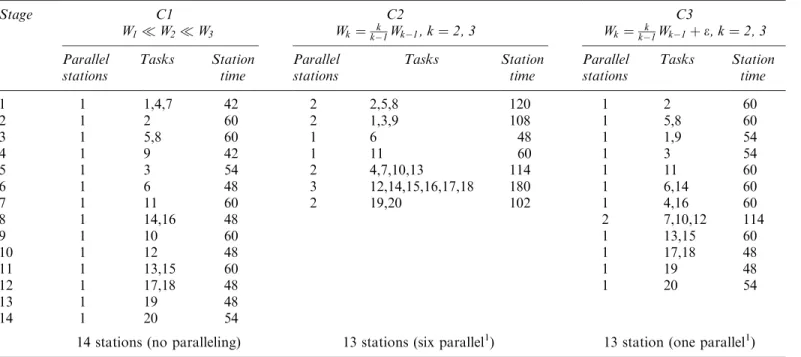
durations in the second column are equal to half of the time in the first column. The same rule is applied to a stage with three parallel stations, and the resulting task times are presented in the third column. It is important to note that the decision on how many parallel stations are allowed may be made for each taskseparately. The de-signer may decide that some of the tasks require expen-sive assembly equipment, and therefore, in order to avoid equipment duplication, they should be performed in a single station. In this case, he can leave the task duration times in the second and third column empty, allowing such tasks to be assigned only to a single sequential sta-tion. The problem was optimally solved for three sets of weights, and the solutions are presented in Table 1.
The solution of each problem is presented in three columns: the first includes the number of stations with and without paralleling, the second consists of the task assignments to stations, and the third presents the accu-mulated assembly time assigned to each station. Case C1 includes a set of weights whereW1 W2 W3(the values of 100, 2000 and 30 000 were chosen here but any other values that satisfy the above condition could be used as well), which imposes a solution without stations in par-allel, resulting in a configuration of 14 stations. Case C2 represents indifference between parallel and sequential stations, by weighting each stage proportionally to its capacity, Wk¼ ðk=k1ÞWk1 (using the weight values 100, 200 and 300). In this case the objective is to minimize the capacity (total number of stations), while being in-different to whether sequential or parallel stations are used. The solution obtained includes 13 stations, most of them in parallel. This solution is an improvement to the solution of C1, but some of the parallel stations may not be essential. In case C3, we use an objective function with a small penalty for the paralleling situation, in favor of solutions with sequential stations (the penalty used is e¼1, resulting in weight values of 100, 201, 302.5). In-deed, the resulting solution includes 13 stations, as in the solution of C2, but with fewer paralleling situations (only one parallel station instead of six parallel stations in C2).
4.2.Long task constraints
Parallel stations are essential where there are tasks with a duration longer than the required cycle time. Consider for example a final assembly line of televisions, where in one of the last stages the TV set should be operated for a couple of hours as a testing phase. It is clear that if a single sequential station will be used at this stage, the testing phase will be the bottleneck of the line, and will cause low throughput and high idle time in other stations. In the actual TV assembly environment, we will probably find at this stage many TV sets being tested in parallel, implementing a situation of many stations in parallel. Figure 2 shows such a situation, where stage j is the testing stage, and the line cycle time isCtime units.
The capacity of stagejismtimesC, where there arem stations in parallel. If, for example, the line daily throughput is 200 TV sets in an 8 hours shift (the cycle time is equal to 2.4 minutes), and the testing time required for each TV is 2 hours, then 50 stations of type j are required to prevent blockage in stagej and meet the re-quired production rate.
By making small changes in the input data of the previous example, we can illustrate the paralleling situa-tion with tasks having a durasitua-tion longer than the required cycle time. Let the duration of task 10 be 72 time units and the duration of task 17 be 90 time units. Both tasks are now longer than the cycle time (60 time units). In this modified problem, a feasible solution must include
par-allel stations to meet the required cycle time. Yet, by applying the different weight factors to control design objectives, three different objective functions can be achieved, as presented by the cases in Table 2.
In case C4, the problem objective enforces only essen-tial paralleling, as required to meet the cycle time by the long tasks. As a result, the optimal solution includes only two parallel stations, one in stage 9 that performs task 10 (along with task 12), and the other in stage 11 that per-forms task 17 (along with task 18). A total of 15 stations are established in the solution of case C4. Case C5 is equivalent to case C2, where the objective is to minimize capacity subject to a given cycle time, a configuration of up to three stations in parallel is allowed, and there is
indifference between stations in parallel and sequential stations. The solution for this case includes five sets of parallel stations and 14 stations in total, one station less than in the solution for case C4. The solution of case C6, in which a small penalty is applied for using parallel stations (as in case C3), also has a total of 14 stations as in C5, but there are only two sets of parallel stations, with three identical stations in each set. The two sets of parallel stations resolve the problem posed by tasks 10 and 17, that have times longer than the cycle time.
These examples illustrate the way in which the weight (cost) parameters can be used in order to change the design objective of the problem to be solved. This use provides the line designer with the flexibility to review solutions for different design objectives, for a wide range of problems involving parallel stations. The different de-sign objectives are all represented by the same model (in which only the weight parameters are modified), and as a result the branch and bound algorithm designed for
solving this model is capable of handling a wide range of problems.
4.3.The effect of the problem parameters on the balancing improvement
In this section we examine how different problem para-meters influence the balancing improvement that can be achieved by using parallel stations. The purpose of this examination is to check the potential for improvement of the line efficiency, by using parallel stations, for a wide range of problems with different characteristics. All ex-periments were performed for problems with 20 tasks, and four factors were defined for the experimentation:
1. F-ratio: The F-ratio is a measure for the flexibility in creating different assembly sequences for aKelements assembly task. It was described by Dar-El (1973), and can be defined as follows:
Letpij be an element of a precedence matrixP, such that:
pij ¼ 1 if taski precedes taskj, 0 otherwise.
n
Then, F-ratio¼2Z=nðn1Þ, where Z is the number of zeroes inP, and nis the number of assembly tasks. The F-ratio value is therefore between zero, when there are no precedence constraints between tasks (any sequence is feasible), and one, when only a single as-sembly sequence is feasible. Asas-sembly tasks are often characterized by relatively low F-ratios. Hence,
pre-Table 1. Optimal solutions of the example problems C1–C3
Stage C1 C2 C3 W1W2W3 Wk ¼k1k Wk1,k¼2, 3 Wk¼k1k Wk1þe,k¼2, 3 Parallel stations Tasks Station time Parallel stations Tasks Station time Parallel stations Tasks Station time 1 1 1,4,7 42 2 2,5,8 120 1 2 60 2 1 2 60 2 1,3,9 108 1 5,8 60 3 1 5,8 60 1 6 48 1 1,9 54 4 1 9 42 1 11 60 1 3 54 5 1 3 54 2 4,7,10,13 114 1 11 60 6 1 6 48 3 12,14,15,16,17,18 180 1 6,14 60 7 1 11 60 2 19,20 102 1 4,16 60 8 1 14,16 48 2 7,10,12 114 9 1 10 60 1 13,15 60 10 1 12 48 1 17,18 48 11 1 13,15 60 1 19 48 12 1 17,18 48 1 20 54 13 1 19 48 14 1 20 54
14 stations (no paralleling) 13 stations (six parallel1) 13 station (one parallel1)
1
Note: the number of parallel stations countsadditionalidentical stations used in parallel with the ‘base’ station (e.g., one parallel station indicates the existence of two identical stations at the stage).
cedence diagrams with F-ratios of 0.1, 0.3 and 0.5 were generated in this study.
2. Average number of tasks per station (ATS): This para-meter is equal to the ratio between the number of tasks in the assembly and the minimal number of stations required to meet the production rate. (The number of stations can be calculated by the ratio of total as-sembly time required and the cycle time.) The pa-rameter was set to two and four tasks per station. 3. Variability of task duration (VTD): The duration of
every task was generated from a uniform distribution. We examined a distribution with a small variance,
Uð0:8l, 1:2lÞ, and a distribution with a high variance
Uð0:4l, 1:6lÞ, wherelis the expected value of the task duration.
4. Maximal number of stations in parallel (MSP): Each problem was solved for a maximal number of two, three and four parallel stations.
For each experiment, three different precedence dia-grams were generated, each with two instances of task durations (total of six replications). In the first set of experiments, the effect of the first three parameters on the balancing improvement is examined. The dependent variable, the balancing improvement, is equal to the ratio between the number of stations obtained with paralleling and the number of stations obtained with no parallel stations. Since an optimal solution was obtained for both cases, this value is always smaller than or equal to one.
Table 3 shows the ANOVA results, where the rows in bold type denote the significant factors (p-value smaller than 0.05). We can see that the effect of the F-ratio and ATS is quite significant, as well as the interaction of the two. As can be expected, the results show that parallel stations are mostly desired in situations where a good balance is difficult to achieve (low F-ratio and small cycle time).
Table 2. Optimal solutions of the example problems C4–C6
Stage C4 C5 C6 W1W2W3 Wk ¼k1k Wk1,k¼2, 3 Wk¼k1k Wk1þe,k¼2, 3 Parallel stations Tasks Station time Parallel stations Tasks Station time Parallel stations Tasks Station time 1 1 1,4,7 42 2 2,5,8 120 1 2 60 2 1 2 60 2 1,3,9 108 1 5,8 60 3 1 5,8 60 1 11 60 1 1,9 54 4 1 9 42 3 4,6,7,10,13 174 1 3 54 5 1 3 54 1 12,14 60 1 11 60 6 1 6 48 3 15,16,17,18 180 3 4,6,7,10,13 174 7 1 11 60 2 19,20 102 1 12,14 60 8 1 14,16 48 3 15,16,17,18 180 9 2 10,12 120 1 19 48 10 1 13,15 48 1 20 54 11 2 17,18 108 12 1 19 48 13 1 20 54
15 stations (two parallel) 14 stations (seven parallel1) 14 stations (four parallel1)
1Note: the number of parallel stations counts additional identical stations used in parallel with the ‘base’ station (e.g., one parallel station indicates
the existence of two identical stations at the stage).
Table 3. ANOVA table of the balancing improvement
General MANOVA Summary of all effects; 1-F-ratio, 2-ATS, 3-VTD
Effect df effect MS effect df error MS error F-ratio p-value
1 2 0.015 750 204 0.003 749 4.2013 0.016 292 2 1 0.595 439 204 0.003 749 158.8323 0.000 000 3 1 0.000 329 204 0.003 749 0.0879 0.767 198 12 2 0.022 669 204 0.003 749 6.0469 0.002 810 13 2 0.004 240 204 0.003 749 1.1309 0.324 755 23 1 0.002 893 204 0.003 749 0.7718 0.380 686 123 2 0.001 009 204 0.003 749 0.2692 0.764 257
Looking at Fig. 3, which demonstrates the F-Ratio-ATS interaction, we can see that the effect of the F-ratio seems much more significant for small ATS. No clear effect is identified for large ATS (in particular we can see that at the upper plot in Fig. 3). The reason for this may be that for relatively large ATS values good balance may be obtained without allowing parallel stations, and the improvement due to paralleling is very small (less than 6% in our experiments). In this small range the effect of the F-ratio is minor. In small ATS, on the other hand, good balance is difficult to achieve, and the effect of the F-ratio is much clearer.
We also examined the effect of the limitation on the number of parallel stations on the balancing improve-ment. Seventy-two problems were solved for each limi-tation, giving a total of 288 problems. The graph in Fig. 4 shows the balancing improvement as a function of the maximal number of parallel stations allowed.
Each point of the graph represents an average value of the 72 problems solved. We can see that the marginal
contribution of the paralleling to the balance solution decreases with the number of parallel stations. In fact, we can say that in this case the significant contribution is obtained for adding the first parallel station (average improvement of 8.4%), and there is very little contribu-tion beyond that (addicontribu-tional improvement of 0.95 and 0.26% for adding the second and third parallel stations respectively). We can assume that those values are de-pendent on the problem parameters, and that another problem set may have resulted in different values of the improvements. However, the trend is quite intuitive, and we can assume that this behavior of the balancing im-provement will remain the same for almost any set of problems. We then may conclude that when the reason for paralleling is balancing improvement we should start solving the problem for a small value of the maximal number of parallel stations, and then increase this value until no significant improvement is obtained.
5. Modification to the multi-equipment line balancing problem with paralleling
The equivalence between the line balancing problem with paralleling and a special case of the line balancing prob-lem with equipment selection was discussed in Section 2. In this section the integration of the two problems is addressed, and an example is given.
Assume that there are moptional equipment types to be assigned to stations. In each stage we can assign either a single piece of equipment or several identical ment units. The problem is to select the required equip-ment type for each stage and the number of parallel stations containing this equipment, and to assign the tasks to stations. The objective is to minimize the total equipment costs. A few notations should be defined for the formulation of the multi-equipment problem with paralleling:
Wkm= the cost of k parallel stations with identical equipment typem;
tim = the duration of task i when performed by equip-ment type m;
yjkm =
1 if there are exactlyk parallel stations in stagejwith equipment type m,
0 otherwise; 8
< :
xijm =
1 if taski is performed by equipment type at stage j,
0 otherwise; 8
< :
M = the number of different equipment types.
The new formulation of the problem (P3) is then:
ðP3Þ minX Jmax j¼1 X Kmax k¼1 XM m¼1 Wkmyjkm; ð1aÞ
Fig. 3. Balancing improvement as a function of the F-ratio and
the ATS.
Fig. 4. Balancing improvement as a function of the paralleling
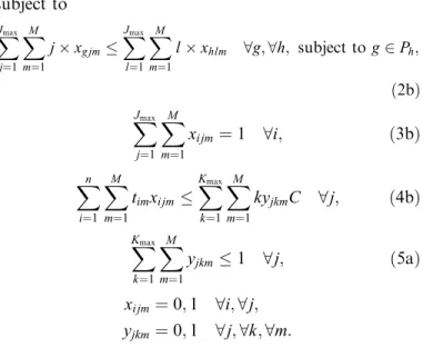
subject to XJmax j¼1 XM m¼1 jxgjm XJmax l¼1 XM m¼1 lxhlm 8g;8h; subject tog2Ph; ð2bÞ XJmax j¼1 XM m¼1 xijm ¼1 8i; ð3bÞ Xn i¼1 XM m¼1 timxijm X Kmax k¼1 XM m¼1 kyjkmC 8j; ð4bÞ X Kmax k¼1 XM m¼1 yjkm1 8j; ð5aÞ xijm¼0;1 8i;8j; yjkm¼0;1 8j;8k;8m:
The formulation is a modification of original formu-lation of the assembly line balancing with paralleling (P1). The objective function (1a) expresses the total equipment cost of the assembly system. Constraint sets (2b), (3b), (4b) and (5a) replace constraint sets (2), (3), (4) and (5) respectively.
The line balancing problem with multi-equipment and paralleling can be solved by the branch and bound al-gorithm, which was presented in Section 3. The weights in the objective function in addition of being control pa-rameters have now also a practical meaning of the equipment costs. In order to demonstrate the identical solving procedure of both problem types, the following example is presented.
An assembly line has to be balanced for a product containing 30 assembly tasks while minimizing the equipment costs. The precedence diagram of the product is presented in Fig. 5. The line cycle time is 250 time units, as derived from the required production rate.
Three equipment types are available for each station:
1. Equipment type M: A highly flexible piece of equip-ment, namely, a piece of equipment that is capable of
performing a large number of assembly tasks (all tasks in this example). A special case of this equipment type may be a human being, which will be considered from now on without loss of generality.
2. Equipment type E1: A fast assembly piece of equip-ment characterized by short tasks’ duration.
3. Equipment typeE2: The least expensive equipment.
The maximal number of parallel station of equipment typesM, E1, and E2 in each stage was set to three, two, and two respectively. The input data of the task duration, which is presented in Table 4 also refers to the maximal number of parallel stations of each equipment type.
Columns ‘M1’, ‘M2’ and ‘M3’ refer to task durations in a single station, two and three parallel stations of the hu-man worker; columns ‘E1
1’ and ‘E12’ refer to a single sta-tion and two parallel stasta-tions of equipment typeE1, and columns ‘E2
1’ and ‘E22’ refer to a single station and two parallel stations of equipment type E2. In this example, every task may be performed in parallel stations where the maximal number of parallel stations is limited by the equipment. In general, we can limit the maximal number of parallel stations for each task independently by en-tering empty cells in the appropriate places in the dura-tion matrix. We can see that the duradura-tion of three out of the 30 tasks (tasks 7, 18 and 28) is larger than the cycle time for all optional equipment types, namely, all feasible configurations should include parallel stations.
The costs of the human worker and the two equipment types are $100 000, $100 000 and $60 000 respectively. (It should be noted that although the cost of the human worker is different than the cost of automated assembly equipment, both can be translated into a total cost over the life cycle of the assembly system.)
The problem was solved according to case C6 (see Table 2), where tasks longer than the cycle time exist and the weights’ values are set according to Equation (6). In this case the minimal equipment costs is obtained in the optimal solution with a minimal number of parallel sta-tions.
An optimal solution for the problem was obtained, and the minimal cost configuration is shown in Fig. 6. The
assembly line contained 10 stages; seven stages include a single station and thee stages include two parallel sta-tions. All optional equipment is used, where in four stages (six stations) a manual worker is assigned, in four stages (five stations) the less expensive equipment is assigned and in other two stages (three stations) the fast equipment is selected.
The quantitative data of the optimal solution are pre-sented in Table 5. The first three columns show the stage number, the selected equipment for each stage and the number of stations in each stage. The assembly tasks assigned to each stage are presented in the fourth column, and not surprisingly we can see that all three tasks with a duration larger than the cycle time (tasks 7, 18 and 26) are assigned in stages with two parallel stations (stages 4, 6 and 8). The accumulated time in each station appears in
the fifth column where in stages with parallel stations the effective station time, defined as the division of the ac-cumulated station time by the number of station, appears in the parenthesis. The equipment cost of each stage is shown in the sixth column and the total equipment costs, $1100 000 is presented at the bottom.
6. Summary and conclusions
The assembly line design with station paralleling and equipment selection has been addressed in this paper. After presenting the basic formulation of the station paralleling, a modified model that takes into consider-ation costs associated with the trade-off between serial and parallel stations is presented. Changing the costs parameters enables us to address a typical assembly line design problem, in which the assembly system may be labor or equipment intensive and where tasks may be larger than the cycle time. An analogy between the par-allel station problem and the assembly system design with equipment selection is shown, where the former problem is found to be a special case of the latter. The advantage
Table 4. Task duration
M1 M2 M3 E11 E12 E12 E22 Task 1 54 27 18 64 32 Task 2 144 72 48 70 35 Task 3 138 69 46 160 80 Task 4 144 72 48 86 43 142 71 Task 5 24 12 8 Task 6 102 51 34 Task 7 300 150 100 380 190 Task 8 114 57 38 58 29 108 54 Task 9 36 18 12 14 7 Task 10 114 57 38 70 35 110 55 Task 11 84 42 28 Task 12 72 36 24 44 22 Task 13 72 36 24 28 14 70 35 Task 14 24 12 8 12 6 Task 15 90 45 30 Task 16 72 36 24 42 21 Task 17 60 30 20 68 34 Task 18 360 180 120 Task 19 36 18 12 42 21 Task 20 114 57 38 64 32 Task 21 96 48 32 86 43 Task 22 24 12 8 14 7 Task 23 30 15 10 30 15 Task 24 78 39 26 48 24 Task 25 12 6 4 12 6 Task 26 270 135 90 290 145 Task 27 78 39 26 50 25 94 47 Task 28 90 45 30 Task 29 150 75 50 154 77 Task 30 36 18 12 22 11
of this observation is two-fold; a solution approach for the equipment selection problem can be used for solving the parallel station problem, and moreover, the two problems can be combined and be efficiently solved. The balancing improvement associated with applying parallel stations is examined through a wide range of experiments. Results show that the flexibility in the order of the as-sembly operations (expressed by the F-ratio measure) and the cycle time (expressed by the ATS measure) have sig-nificant effects on the balancing improvement. We can state that parallel stations are especially needed when a good balance is difficult to obtain due to small cycle times or low flexibility in the assembly process. Another inter-esting observation concerns the relationship between the paralleling limitation (maximal number of stations in parallel in a single stage) and the balancing improvement. Results show that the first station in parallel contributes the main improvement (8.4% on average) while the contribution of additional parallel stations is quite small (0.95 and 0.26% are associated with the third and fourth parallel stations respectively). The importance of this observation results from the fact that the branch and bound algorithm run time is highly dependent on this parameter. For practical problems, based on this result of diminishing returns one may experiment with low values (of one or two) stations in parallel. In cases where many parallel stations are needed due to long task times, such as in the testing stage of the TV line example, it will be reasonable to solve this part of the problem separately, without combining additional tasks with short task times into such stations.
The combined problem, which incorporates the station paralleling with equipment selection problem is discussed in the paper, an ILP formulation is developed and an optimal solution of an example problem is presented. We believe that the design approach presented here is suitable for handling various practical problems. Nevertheless, much further research should be done in combining more aspects of practical design problem, such as the
multi-mixed-model environment, stochastic assembly times and machine breakdown.
Acknowledgement
This work was performed in part while Dr. Bukchin was on a sabbatical at the Grado Department of Industrial and Systems Engineering, Virginia Tech, and Dr. Rubi-novitz was on leave at the Department of Industrial En-gineering, Tel Aviv University. The authors wish to thank both departments for the hospitality during their stay.
References
Askin, R.G. and Zhou, M. (1997) A parallel station heuristic for the mixed-model production line balancing problem. International Journal of Production Research,35(11), 3095–3105.
Bard, J.F. (1989) Assembly line balancing with parallel workstations and dead time. International Journal of Production Research,
27(6), 1005–1018.
Baybars, I. (1986) A survey of exact algorithms for the simple assem-bly line balancing problem.Management Science,32(8), 909–932. Bukchin, J. and Tzur, M. (2000) Design of flexible assembly line to
minimize equipment cost.IIE Transactions,32(7), 585–598. Buxey, G.M. (1974) Assembly line balancing with multiple stations.
Management Science,20(6), 1010–1021.
Dar-El, E.M. (1973) MALB - A heuristic technique for balancing large single-model assembly lines.AIIE Transactions,5(4), 343–356. Erel, E. and Sarin, S.C. (1998) A survey of assembly line balancing
procedures.Production Planning and Control,9(5), 414–434. Ghosh, S. and Gagnon, R.J. (1989) A comprehensive literature review
and analysis of the design, balancing and scheduling of assembly systems.International Journal of Production Research,27(4), 637– 670.
Mastor, A. (1970) An experimental investigation and comparative evaluation of production line balancing techniques.Management Science,16(22), 728–745.
McMullen, P.R. and Frazier, G.V. (1997) Heuristic for solving mixed-model line balancing problems with stochastic task durations and parallel stations.International Journal of Production Economics,
51(3), 177–190.
McMullen, P.R. and Frazier, G.V. (1998) Using simulated annealing to solve a multiobjective assembly line balancing problem with
par-Table 5. Optimal solution
Stage Equipment type Number of stations Tasks Acc. time Cost (·$000)
1 E2 1 1,2 224 60 2 M 1 5,6,9 234 100 3 E1 1 2,4,10 226 100 4 E2 2 7,8 488 (244) 120 5 M 1 11,15,17 234 100 6 M 2 14,18,20 498 (249) 200 7 E2 1 13,21,23 186 60 8 M 2 16,19,22,24,25,26 492 (246) 200 9 E2 1 27,29 248 60 10 M 1 28,30 126 100 Total cost: (·$000) $1100
allel workstations.International Journal of Production Research,
36(10), 2717–2741.
Nanda, R. and Scher, J.M. (1975) Assembly lines with overlapping work stations.AIIE Transactions,7(3), 311–318.
Nanda, R. and Scher, J.M. (1976) Nonparallelability constraints in assembly lines with overlapping work stations.AIIE Transactions,
8(3), 343–349.
Pinnoi, A. and Wilhelm, W.E. (1997) Family of hierarchical models for the design of deterministic assembly systems.International Journal of Production Research,35(1), 253–280.
Pinnoi, A. and Wilhelm, W.E. (1998) Assembly system design: a branch and cut approachManagement Science,44(1), 103–118. Pinto, P., Dannenbring, D.G. and Khumawala, B.M. (1975) A branch
and bound algorithm for assembly line balancing with paralleling.
International Journal of Production Research,13(2), 183–196. Pinto, P., Dannenbring, D.G. and Khumawala, B.M. (1981) Branch
and bound heuristic procedures for assembly line balancing with paralleling of stations. International Journal of Production Re-search,19(4), 565–576.
Suer Gursel, A. (1998) Designing parallel assembly lines.Computers and Industrial Engineering,35(3–4), 467–470.
Sarker, B.R. and Shantikumar, J.G. (1983) Generalized approach for serial or parallel line balancing.International Journal of Produc-tion Research,21(1), 109–133.
Talbot, F.B., Patterson, J.H. and Gehrlein, W.V. (1986) A comparative evaluation of heuristic line balancing techniques. Management Science,32(4), 430–454.
Udomkesmalee, N. and Daganzo, C.F. (1989) Impact of parallel processing on job sequences in flexible assembly systems. Inter-national Journal of Production Research,27(1), 73–89.
Biographies
Joseph Bukchin is a faculty member of the Department of Industrial Engineering at Tel Aviv University. He received his B.Sc., M.Sc. and D.Sc. degrees in Industrial Engineering from the Technion, Israel In-stitute of Technology. He is a member of the IIE and INFORMS. He was a visiting professor at the Grado Department of Industrial and Systems Engineering at Virginia Tech. His main research interests are in the areas of assembly systems design, assembly line balancing, fa-cility design, design of cellular manufacturing systems, operational scheduling as well as work station design with respect to cognitive and physical aspects of the human operator.
Jacob Rubinovitz is a Senior Lecturer at the Faculty of Industrial Engineering and Management of the Technion. He holds a B.Sc and M.Sc. in Industrial Engineering from the Technion, and a Ph.D. in Industrial Engineering from The Pennsylvania State University. He is a senior member of the Institute of Industrial Engineers (IIE), the Society of Manufacturing Engineers (SME), and the Israel Society for Com-puter Aided Design and Manufacturing. He established the Robotics and Computer Integrated Manufacturing Lab at the Faculty of In-dustrial Engineering and Management at the Technion, and served as its head between 1988–1995. He has held visiting appointments at the Industrial Engineering departments of the University of Pittsburgh (1995–1996) and the Tel Aviv University (2001–2002). The research focus of Dr. Rubinovitz is optimization of design and operation of flexible computer-integrated manufacturing systems and assembly systems.