Exchange Rate Predictability in a Changing World *

Exchange Rate Predictability in a Changing World

Joseph P. Byrne

, Dimitris Korobilis

, and Pinho J. Ribeiro

February 14, 2014

Abstract

An expanding literature articulates the view that Taylor rules are helpful in predicting

exchange rates. In a changing world however, Taylor rule parameters may be subject to

structural instabilities, for example during the Global Financial Crisis. This paper

forecasts exchange rates using such Taylor rules with Time Varying Parameters (TVP)

estimated by Bayesian methods. In core out-of-sample results, we improve upon a

random walk benchmark for at least half, and for as many as eight out of ten, of the

currencies considered. This contrasts with a constant parameter Taylor rule model that

yields a more limited improvement upon the benchmark. In further results, Purchasing

Power Parity and Uncovered Interest Rate Parity TVP models beat a random walk

benchmark, implying our methods have some generality in exchange rate prediction.

Keywords

: Exchange Rate Forecasting; Taylor Rules; Time-Varying Parameters;

Bayesian Methods.

JEL Classification

: C53, E52, F31, F37, G17.

*_{Corresponding author at: Department of Economics, University of Glasgow, UK. Email address:}

[email protected], Tel: +44 (0)141 330 2950. Fax.: +44 (0)141 330 4940.

a _{Department of Economics, Heriot-Watt University, Edinburgh, UK.} b

Department of Economics, Adam Smith Business School, University of Glasgow, Glasgow, UK.

1

1.

Introduction

Academics and market practitioners have long sought to predict exchange rate

fluctuations. A long held view, initiated by Meese and Rogoff (1983), proposed that

forecasts based upon macroeconomic fundamentals could not improve upon a random walk

benchmark, especially at short horizons. Rossi (2013) provides a survey of a subsequent

literature that achieved successes in improving upon the benchmark, using theoretical and

empirical innovations. Theoretical improvements have included utilising asset pricing

models and Taylor rules and, separately, empirical advances have included nonlinear

methods.

This paper seeks to combine these theoretical and empirical innovations in

predicting exchange rates, in a changing world.

Engel and West (2005) and Engel et al. (2008) illustrate that models that can be cast

in the standard present-value asset pricing framework imply that exchange rates are

approximately random walks. This holds under the assumptions of non-stationary

fundamentals and a near unity discount factor. However, Engel and West (2004) present

evidence that even when the discount factor is near one, a class of models based on

observable fundamentals can still account for a fairly large fraction of the variance in

exchange rates. An example in this class includes structural exchange rate models in which

monetary policy follows the Taylor (1993) rule. Indeed, Engel et al. (2008), Molodtsova

and Papell (2009) and Rossi (2013) find that empirical exchange rate models conditioned

on an information set from Taylor rules outperform the random walk benchmark in

out-of-sample forecasting, especially at short-horizons.

Despite the optimism instilled by this emerging research, one area remains

unresolved. This is the frequent regularity that exchange rate predictability is often

sample-dependent, and hence forecasting ability appears in some periods but not in others. Rogoff

and Stavrakeva (2008) and Rossi (2013) examine these issues thoroughly. Rogoff and

Stavrakeva (2008) show for instance that Molodtsova and Papell’s (2009) results may

change in a different forecast window. Rossi (2013) also finds that models’ predictive

power is specific to some currencies in some periods but not others. In fact, she concludes

by questioning whether instabilities can be explored to improve exchange rates forecasts.

For nonlinear models, see Wolff (1987), Sarno et al. (2004), Rossi (2006), Bacchetta et al. (2010), Balke et al. (2013) and Park and Park (2013). Other empirical approaches have included: long-horizon methods, see Mark (1995); panel models, see for example Papell (1997), Groen (2000), MacDonald and Nagayasu (2000), Mark and Sul (2001) and Engel et al. (2008); and factor exchange rate models, see Engel et al. (2012).

2

There are several reasons to examine the hypothesis that exchange rate

predictability is dependent on instabilities in regression and policy coefficients. Firstly,

research shows that macroeconomic conditions and policy actions evolve, often suddenly.

Boivin (2006), Kim and Nelson (2006) and Cogley et al. (2010) present evidence that the

U.S. Federal Reserve's conduct of monetary policy is better characterized by a

changing-coefficients Taylor rule. Trecoci and Vassali (2010) present similar evidence for the U.S.,

U.K., Germany, France and Italy. Secondly, there is widespread evidence of a

time-evolving relationship between exchange rates and fundamentals. Bacchetta and van

Wincoop (2004), for example, explain this relationship on the basis of a scapegoat theory.

Foreign exchange traders often seek explanations for fluctuations in the exchange rate, such

that even when an unobservable is responsible for the actual change, it is common to

attribute it to an observable macro variable or the scapegoat. Subsequently, this scapegoat

variable influences trading behaviour and the exchange rate. Over time, fluctuations in

exchange rates are then explained by time-varying weights attributed to scapegoat

variables. In a recent application, Balke et al. (2013) and Park and Park (2013) show that

allowing for such type of coefficient adaptivity in an monetary model improves in-sample

fit and out-of sample predictive power for exchange rates.

It is timely and topical to exploit non-linear Taylor rules when predicting

exchange rates. While an extensive literature focuses on linear and non-linear models with

standard fundamentals based models, there is limited research focusing on the predictive

ability of non-linear Taylor rules.

Non-linear methods are pertinent given the nature of the

world economy during the last decade. Taylor (2009) argues that before the Global

Financial Crisis the U.S. Fed’s conduct of monetary policy was characterized by deviations

from a linear Taylor rule. After the Crisis, Central Banks around the world have adopted

unconventional monetary policy, also inconsistent with linear Taylor rules. Hence we look

afresh at Taylor rules predictive content against a random walk.

2 _{See for example, Stock and Watson (1996) for evidence on structural instabilities in macroeconomic time}

series in general.

3

Rossi (2013) provides an excellent survey of recent work using linear and non-linear Purchasing Power Parity, Monetary Model and Uncovered Interest Rate Parity. Papers that focus on Taylor rule predictive content in a linear modelling framework include, Engel and West (2004, 2005, 2006), Engel et al. (2008), Rogoff and Stavrakeva (2008) Molodtsova et al. (2008) and Molodtsova and Papell (2009, 2013). For non-linear modelling of Taylor rules, Mark (2009) is a notable contribution. He employs a Vector Autoregressive model and least-squares learning techniques to update Taylor rules estimates, inflation and output gap which are then then used to compute the exchange rate value. Using in-sample evidence, he finds that allowing for time-variation in parameters is relevant to account for the volatility of the Deutschemark and the Euro, relative to the U.S dollar. Our approach differs from Mark (2009) in that we focus upon out-of-sample predictability of non-linear Taylor rules.

3

This paper's main contribution is to predict exchange rates accounting for

parameter instabilities in Taylor rules by using Bayesian methods. Previous studies, such as

Molodtsova and Papell (2009), Engel et al. (2008), Rossi (2013), among others, assumed

constant coefficients in the Taylor rules, along with constant coefficients in the forecasting

regression. These restrictions about the degree of parameter adaptivity may rationalize the

difficulty in pining down model’s forecasting performance over-time. Our hypothesis is

that the predictive content might be time-varying because fundamentals themselves and

their interaction with exchange rates change over time. In light of this, we estimate

time-varying parameter Taylor rules and examine their predictive content in a framework that

also allows for the parameters of the forecasting regression to change over time.

In a major

break with the earlier non-linear exchange rate literature, we estimate time varying

parameters using information in the likelihood based upon Bayesian methods. Therefore,

we do not rely on calibration (e.g. Wolff, 1987; Bacchetta et al., 2010), which can be

subjective and may give less accurate parameter estimates and inferior forecasting

performance.

In particular, this paper's dataset consists of quarterly exchange rates from 1973Q1

to 2013Q1, on up to 17 OECD countries relative to the U.S. dollar. We calculate Theil’s U

statistic from Root Mean Squared Forecast Error (RMSFE) recursively out-of-sample,

whilst using three forecasting windows. To preview our results, allowing for time-varying

Taylor rules improves upon the driftless random walk at both short and long horizons. In

fact, in most forecast windows our approach yields a lower RMSFE than the benchmark for

at least half of the currencies in the sample. We improve upon the benchmark for as many

as 11 out of 17 currencies in our earlier forecast window, and eight out of 10 in our latest

forecast window. Hence, the predictive ability is particularly robust to the recent Financial

Crisis.

This paper also contributes to the literature by forecasting using panel methods

and Bayesian time-varying parameters regressions conditioned on the standard predictors

4 _{Although in principle forecasting using a rolling regression scheme as in Molodtsova and Papell (2009,}

2013) allows for instability to be taken into account, a TVP model allows for instabilities to be updated systematically. We also note that while formal tests of parameter instabilities could be conducted in-sample, our approach relies on verifying the plausibility of time-variation in the relationships by means of out-of-sample forecast evaluation.

5 _{Giannone (2010) provides a helpful critique of the results based on Bacchetta’s et al.(2010) calibration, and}

shows how using the full maximum likelihood setup in a Bayesian framework is important in accounting for instabilities. Balke et al. (2013) also use Bayesian methods and focus upon modelling exchange rates in-sample with monetary fundamentals.

4

from Purchasing Power Parity (PPP), a Monetary Model (MM), Uncovered Interest Rate

Parity (UIRP) and Engel et al. (2012) factor model. The TVP forecasting regression also

performs relatively well for over half of the currencies in most windows, when conditioned

on PPP at all horizons and UIRP at long-horizon. The panel model generates lower RMSFE

than the benchmark for half or more currencies across windows when based on PPP and

factors at all horizons, and Taylor rules and UIRP for long-horizon forecasts. However,

results for the panel regression are only robust for PPP at all horizons and factors at longer

horizons. The predictive content of the MM is less promising for our quarterly sample

period, regardless of the forecasting model.

The rest of the paper proceeds as follows. The next section sets out the

Time-Varying Parameter regression we consider. Section 3 discusses the choice of fundamentals,

and Section 4 covers data description and the mechanics of our forecasting exercise. The

main empirical results are reported in Section 5. Section 6 deals with robustness checks and

the final Section concludes.

2.

The Time-Varying Parameter Regression

A common practice in forecasting exchange rates is to model the change in the

exchange rate as a function of its deviations from its fundamental implied value. As put

forward by Mark (1995), this accords with the notion that exchange rates frequently deviate

from their fundamental implied value, particularly in the short-run. More precisely, define

as the h-step-ahead change in the log of exchange rate, and

a set of

exchange rate fundamentals. Then,

(1)

where,

(2)

As (1) suggests,

signals the exchange rate’s fundamental value and hence

, is the

deviation from the fundamental’s implied level. When the spot exchange rate is lower than

the level implied by the fundamentals, i.e.,

, then the spot rate is expected to

increase.

In equation (2), the time-subscripts

attached to the coefficients

[

]

,

make it evident that the regression allows the coefficients to change over time.

The exact

coefficient’s law of motion is inspired, among others, by Stock and Watson (1996), Rossi

5

(2006), Boivin (2006) and Mumtaz and Sunder-Plassmann (2012). We assume a Random

Walk Time-Varying Parameter (RW-TVP). Thus, for

[

]

, the process is:

(3)

where, the error term

is assumed homoscedastic, uncorrelated with

in equation (1)

and with a diagonal covariance matrix

Q

. Putting together equations (1) and (3) results in a

state-space model, where (1) is the measurement equation and (3) the transition equation.

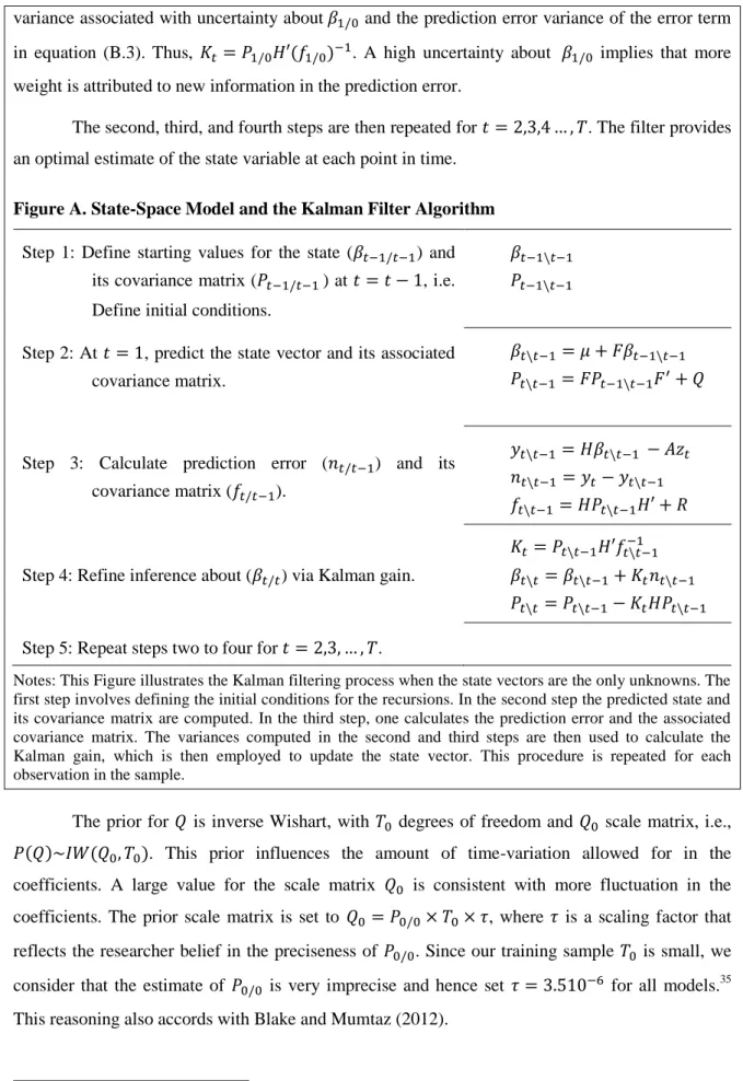
We use Bayesian methods to estimate the parameters of the state-space model.

While the use of the Kalman filter with maximum likelihood is another potential method,

the evaluation of a large number of likelihood functions in this case might undermine the

estimates (Kim and Nelson, 1999). That is, with the method of maximum likelihood there

is potential for accumulation of errors, as estimation of the state variables is conditional on

maximum likelihood estimates of the other parameters of the system. In addition, there are

is also the issue of identifying objective priors to initialize the Kalman filter. Whilst to

address the latter the approach in the literature often involves setting diffuse priors or using

a training sample, solving the problem of obtaining efficient parameter estimates is a more

cumbersome task. By contrast, Bayesian methods treat all the unknown parameters in the

system as jointly distributed random variables, such that the estimate of each of them

reflects uncertainty about the others (Kim and Nelson, 1999).

In particular, we rely on the Carter and Kohn (1994) algorithm and the Gibbs

sampler to simulate draws from the parameters’ posterior distribution. The Gibbs sampler,

which falls within the category of Markov Chain Monte Carlo (MCMC) methods, is a

numerical method that uses draws from conditional distributions to approximate joint and

marginal distributions. More precisely, to fully implement the Bayesian method, we need to

(i) elicit priors for the unknown parameters, (ii) specify the form of their posterior

conditional distributions, and finally (iii) draw samples from the specified conditional

posterior distribution. To parameterize the prior distributions we use pre-sample

information. We do so largely because we are comparing the forecasting performance of

various models, at a number of forecast windows and horizons. By setting priors based on a

training sample we aim at ensuring that all the models are based on the same prior

elicitation setting, and hence their performance is not influenced by the model’s particular

prior parameterization choice. This approach also provides natural shrinkage based on

evidence in the likelihood, which in turn ensures that TVP estimates will be more accurate,

with smaller variance, resulting in a sharper inference and potentially more precise

6

forecasts.

The remainder of the details about priors’ elicitation and all the other steps are

provided in Appendix B.

3.

Choice of Fundamentals

Having defined the form and the method to estimate the parameters of our main

forecasting regression, an additional modelling issue relates to the exact specification of the

fundamental information contained in

. In this regard, our approach is broadly consistent

with models that relate the exchange rate to macroeconomic variables within the asset

pricing framework. In this framework, the exchange rate is expressed as the present-value

of a linear combination of economic fundamentals and unexpected shocks. Under the

assumptions of rational expectations and a random walk time series process for the

fundamentals, the framework implies that the spot exchange rate is determined by current

observable fundamentals and unobservable noise (Engel and West, 2005). We focus

primarily on observable fundamentals derived from the Taylor (1993) rule, MM, PPP,

UIRP, and the co-movement among exchange synthetized by factors from exchange rates.

3.1.1

Taylor Rule Fundamentals

The Taylor (1993) rule postulates that monetary authorities should set the target for

the policy interest rate considering the recent inflation path, inflation deviation from its

target, output deviation from its potential level, and the equilibrium real interest rate. Then,

it follows that they increase the short-term interest rate when inflation is above the target

and/or output is above its potential level. Note that the Taylor principle presupposes an

increase in the nominal policy rate more than the rise in inflation rate to stabilize the

economy.

An emerging research considers the implications of this policy setting for exchange

rates, including Engel and West (2005), Engel et al. (2008), Mark (2009), and Molodtsova

and Papell (2009, 2013). The premise is that the home and the foreign central banks

conduct monetary policy following the Taylor principle. In line with this principle, the

foreign monetary authority, taken as the U.S. in our empirical section, is concerned with

inflation and output deviations from their target values. In addition to these targets and

6 _{In our empirical exercise we also experimented using the Kalman filter with Maximum Likelihood (ML).}

However unlike papers that employ diffuse priors, such as Rossi (2006), we also used data-based priors to initialize the Kalman filter recursions. Our rationale for employing these priors in this case is that while diffuse priors when using ML estimates are objective, they result in larger uncertainty about the TVP estimates, which may lead to loss of forecast power.

7

consistent with historical evidence, Engel and West (2005) assume that the home country

also targets the real exchange rate. It is also common, following Clarida et al. (1998), to

consider that central banks adjust the actual interest rate to eliminate a fraction of the gap

between the current interest rate target and its recent past level, known as interest rate

smoothing. By subtracting the foreign Taylor rule from the home, the following interest

rate differential equation is obtained:

̅

̅

(4)

where

, is the short-term nominal interest rate set by the central bank, asterisks denote

foreign (U.S.) variables;

, is inflation;

̅

, denotes output gap;

is the real exchange rate

defined as

;

, is the log nominal exchange rate, defined as the home

price of foreign currency;

, is the log of the price level;

for

, are

coefficients, and

is the unexpected disturbance term, which is assumed to be Gaussian.

A full derivation of equation (4) is provided in Appendix A.

The link from monetary policy actions to exchange rates occurs through UIRP and

the forward premium puzzle. Molodtsova and Papell (2009) discuss at length such

mechanisms. They note for example that under UIRP and rational expectations, any

circumstance that causes the home central bank to increase its policy rate relative to the

foreign, will lead to an expected depreciation of its currency relative to the foreign country.

Such circumstances include for example an increase in inflation above the target, a rise in

the output gap or a deviation of the real exchange from the target. Conversely, foreign

country’s policy actions characterized by an increase in the interest rate will be followed by

an expected depreciation of its currency. However, the empirical evidence frequently

rejects the UIRP condition and this is known as the forward premium puzzle (Engel, 1996).

In fact, the evidence is that high interest rate currencies tend to appreciate, rather than

depreciate as UIRP posits. This suggests that while we can substitute out the interest rate

differential by the expected change in exchange rate in equation (4) to obtain the exchange

rate forecasting regression, we impose no restrictions on the effect of monetary policy on

exchanges rates.

Using equation (4) to derive the forecasting regression or estimate Taylor rule

fundamentals is valid when parameters are constant over time. In a dynamic world

however, Taylor rule parameters may be subject to structural instabilities. Therefore, rather

than estimating or assuming Taylor rules fundamentals from models with constant or

8

calibrated parameters, we allow for the possibility of monetary policies that respond to

macroeconomic conditions in a time-varying fashion. Hence, we estimate fundamentals

from Taylor rules using a TVP regression of the following form:

̅

̅

(5)

from which we compute the fundamentals as:

̂

̂

̂

̂

̅

̂

̅

̂

̂

̂

(6)

where the time-subscript,

, attached to the coefficients defines time-varying parameters

and the symbol “^” indicates parameter estimates. Note that this is identical to equation (4)

except for the time-varying coefficients. This suggests that both, the information set from

Taylor rules and the exchange rate forecasts, are generated from TVP regressions.

The exact form of the Taylor rule and hence of equation (5) varies depending on a

number of assumptions. We focus on three popular variants.

In all variants the equilibrium

real interest rate and the inflation target of the home and foreign country are assumed to be

identical. Thus, in equation (5) the term

equals zero.

In addition, all specifications are

asymmetric; that is, apart from the inflation and output gaps which both countries target,

the home country also targets the real exchange rate.

With the above assumptions maintained, the first Taylor rule specification further

assumes homogeneous coefficients and no interest rate smoothing – abbreviated as TR

.

This signifies that it imposes equality in the coefficients on inflation (

) and the

output gap (

) of the home and foreign country Taylor rules. In addition, central

banks do not smooth interest rates (

). Engel and West (2006) find that it is

reasonable to assume parameter homogeneity across countries. The assumption of no

interest rate smoothing accords with Engel and West’s (2005) formulation. Molodtsova and

Papell (2009) use an identical Taylor rule.

7 _{We can equivalently express the predictor in terms of - see equation (2). In this case we would have:}

̂ ̂ ̂ ̂ ̅ ̂ ̅ ̂ ̂ ̂ .

8 _{The three variants we consider constitute counterpart to the constant-parameter specifications denoted TR} on

and TRos and TRen in Appendix A. 9

This is a typical assumption in this literature including in Engel and West (2005), Engel et.al (2008), Rogoff and Stavrakeva (2008), and Molodtsova and Papell (2013). As Molodtsova and Papell (2013) note, whether to include a constant that capture differences in the equilibrium real interest rate and inflation target is irrelevant, because the forecasting regression includes a constant. We also opted to drop the constant term following our empirical experiment with Taylor featuring this term. In all cases the coefficient was very small and not significantly different from zero.

9

A second specification is similar to the above, except that it includes lagged interest

rates. Therefore, it is an asymmetric rule, with homogeneous coefficients and interest rate

smoothing (TR

).

Since the assumption of coefficients’ homogeneity between the home

and the foreign country is maintained, then we also have

in equation (5). The

inclusion of lagged interest rates implies that central banks limit volatility in the interest

rates and is in the spirit of Engel et al. (2008), Mark (2009) and Molodtsova and Papell

(2009).

The third variant relaxes the assumption of homogeneous coefficients across

countries made above and central banks do not smooth interest rates. Therefore, in equation

(5),

; and is an asymmetric rule, with heterogeneous coefficients and no

interest rate smoothing (TR

). Molodtsova and Papell (2009) find that models of this type

exhibit a strong forecasting performance.

To estimate each of these variants we set up a state-space representation as in

Section 2, but here the measurement equation is defined by (5) and the transition process

also follows a random walk. That is, as in equation (3) but with

replaced by

. The

estimation procedure is also based on Bayesian methods and details about priors’

elicitation, posterior distributions, and sampling algorithm are provided in Appendix B.

However, we note here that like in the forecasting regression, our results rely on data-based

information to parameterize priors and the initial conditions.

3.1.2

Monetary, PPP, UIRP and Factor Fundamentals

The TVP forecasting regression also uses the content of four alternative sets of

information. These are from the monetary model (MM), PPP condition, UIRP hypothesis,

and factors from exchange rates. In notation:

(

) (

)

(7)

(8)

(

)

(9)

∑

(10)

where, in addition to the variables previously defined,

is the log of money supply;

denotes the log of income;

R

is the number of factors;

is the loading of factor

in the

currency

;

and

is the estimated

factor.

While fundamentals given by identities (7), (8), and (9) are standard in the

exchange rate literature, those represented by the co-movement among exchange rates as in

10

identity (10) have been recently propounded by Engel et al. (2012). Their basic

presumption is that the exchange rate of country

follows the process:

(11)

where,

is the effect of the factor in country’s

exchange rate;

is the respective factor

loading, and

is a country specific shock, which is uncorrelated with the factors. Engel et

al. (2012) show that under plausible assumptions, for example that the common factor

follows a random walk process, the RMSFE of the factor model is lower relative to the

RMSFE of the random walk. In our empirical procedure we follow Engel et al. (2012) and

allow for one, two or three factors, estimated via principal components.

To obtain initial conditions for the forecasting regression, we simply compute for

the initial 20 data-points the series defined by the identity (7) for MM, (8) for PPP, (9) for

UIRP, and extract factors to obtain fundamentals given by (10).

We then use these

fundamentals to estimate a constant-parameter model akin to our forecasting regression,

from which we parameterize the priors, initial states, and the covariance matrices of the

TVP forecasting regression. The observations used to parameterize priors are discarded,

and we use the remaining sample period and the same identities above, (7)-(10), to

compute fundamentals that constitute our predictors in the TVP forecasting regression.

Apart from our main forecasting regression which allows the coefficients to vary

over time, we also forecast with a second regression which maintains them constant; i.e.,

, for

in equation (1).

Engel et al. (2008) find that panel data methods

forecast better than single-equation methods. Accordingly, we also use a Fixed-effect (FE)

panel regression as in Engel et al. (2008, 2012). In this case, except for the Taylor rules, the

set of information from the MM, PPP, UIRP, and factors is computed exactly as in the TVP

forecasting approach, i.e., as in identities, (7)-(10). The information set from Taylor rules

specifications is obtained by estimating, via OLS, a single-equation fixed-parameter model

similar to equation (4). Table 1 summarises all these aspects.

10 _{Engel et al. (2012) estimate the factors using maximum likelihood or principal components, and report}

evidence of fairly comparable results.

11 _{As should be clearer in the next Section, allowing for time-variation in the parameters in a recursive}

forecasting approach implies that there are potentially two sources of variation that will ultimately impact upon the parameters. The first is due to the recursive algorithm when computing the optimal parameter at each time of the in-sample period. The second source arises from extending the sample as observations are added to end of the in-sample period (recursions). Therefore, a TVP model allows for more flexibility and presumably more consistent estimates as the sample is extended. We note as well that the second effect is also prevalent in the constant-parameter forecasting regression.

11

Table 1. Empirical Exchange Rate Models and Forecasting Approaches

Fundamentals-based

Exchange Rate Model

TVP Approach Constant Parameter Approach Forecast Windows and Number of Currencies Considered (N) Information set (Fundamental) Forecasting model Information set (Fundamental) Forecasting model

Taylor Rule (TR)

Estimated with a random walk Time-Varying Parameter model using Bayesian methods: TRon: ( ) ( ̅ ̅ ) TRos: ( ) ( ̅ ̅ ) ( ) TRen: ̅ ̅

Random walk Time-Varying Parameter (TVP) model, estimated using Bayesian methods:

Estimated with a single-equation fixed-parameter model, via Ordinary Least Square estimator: TRon: ( ) ( ̅ ̅ ) TRos: ( ) ( ̅ ̅ ) ( ) TRen: ̅ ̅ Fixed-effect Panel model, estimated via Least Square Dummy Variable estimator: A: 1995Q1-1998Q4; N=17 (all currencies in the sample); B: 1999Q1-2013Q1; N=10 (non-Euro area currencies and the Euro);

C: 2007Q1-2013Q1; N=10 (non-Euro area currencies and the Euro). Monetary Model Computed as : ( ) ( ) Computed as: ( ) ( ) PPP Computed as : Computed as : UIRP Computed as : ( ) Computed as : ( )

Factors Factors estimated through principal components analysis.

Factors estimated through principal components analysis.

Notes: This Table summarizes the models considered and the forecasting approaches. The definition of the variables is as follows: = interest rate; = inflation rate; = output; ̅= output gap; = real exchange rate; = money; = price level; = nominal exchange rate. The subscripts and denote country and time, respectively. Asterisk defines the foreign country. Three variants of Taylor rules (TR) are considered: (i) TRon: asymmetric rule with homogeneous coefficients and no interest rate

smoothing, (ii) TRos: asymmetric rule with homogeneous coefficients and interest rate smoothing) and (iii) TRen: asymmetric rule with heterogeneous coefficients and no

interest rate smoothing. See Appendix A for derivations. The factor model allows for one (F1), two (F2), or three (F3) factors. The forecasts are computed for one-, four-, eight-, and 12-quarters-ahead forecasts.

12

4.

Data and Forecast Mechanics

4.1

Data

The data comprises quarterly figures spanning 1973Q1:2013Q1 from 18 OECD

countries: United States, United Kingdom, Switzerland, Sweden, Spain, Norway,

Netherlands, Korea, Italy, Japan, Germany, France, Finland, Denmark, Canada, Belgium,

Austria and Australia. The main source is the IMF’s (2012)

International Financial

Statistics

(IFS). Some of the countries in our sample period moved from their national

currencies to the Euro. To generate the exchange rate series for these countries, the

irrevocable conversion factors adopted by each country on the 1

of January 1999 were

employed, in the spirit of Engel et al. (2012). The money supply is measured by the

aggregate M1 or M2.

To estimate Taylor rules we need the short-run nominal interest rates set by central

banks, inflation rates and the output gap or the unemployment gap.

We use the central

bank’s policy rates when available for the entire sample period, or alternatively the

discount rate or the money market rate. The proxy for quarterly output is the industrial

production in the last month of the quarter. The output gap and unemployment gap are

obtained by applying the Hodrick and Prescott (1997) filter recursively, to the output and

unemployment series. The price level consists of the consumer price index (CPI) and the

inflation rate is defined as the (log) CPI quarterly change. The data on money supply,

industrial production, unemployment rate and CPI were seasonally adjusted by taking the

mean over four quarters following Engel et al. (2012).

4.2

Forecast Implementation and Evaluation

As noted in the previous Sub-section, the sample covers the period 1973Q1 to

2013Q1. We use the sample period from 1974Q1 to 1978Q4 to parameterize the priors and

initial conditions for the TVP regressions. The in-sample estimation period begins in

1979Q1 for all models, including the fixed-parameter ones.

Exceptions are for Sweden, where M3 is used; Australia -M3; and the UK -M4. See Appendix C for extra details.

16 _{In estimating Taylor rules and due to possible endogeneity issues, several authors emphasize the timing of}

the data employed. The discussion centres on the idea that Taylor rules are forward-looking, and hence ex-post data might reflect policy actions taken in the past. Kim and Nelson (2006) note two approaches that can be employed to account for this. The first comprises using historical real-time forecasts that were available to policy-makers. The second consists in using ex-post data to directly model the policy-makers’ expectations. Since historical real-time forecasts are unavailable for our sample of countries, we follow Molodtsova and Papell’s (2009) approach, and use data that were observed (as opposed to the real-time forecasts) at time t, while forecasting t + h period.

13

Rogoff and Stavrakeva (2008) argue that the predictive ability of

fundamentals-based exchange rate models is often sample-dependent. To verify models’ forecasting

performance in alternative forecast windows we consider three sub-samples.

The first

out-of-sample forecasts are for the period 1995Q1-1998Q4. This corresponds to the

pre-Euro period. Forecasts for all the 17 countries’ currencies are generated and models’

forecast accuracy evaluated. A second forecasting window covers the post-Euro period:

1999Q1-2013Q1. Since we have extended the exchange rates of the Euro-area countries

throughout, the forecast of the Euro currency is computed as an average of the forecasts of

the Euro-area countries in our sample. The forecast error is constructed as the difference

between each of the country’s realized value and the computed average. We therefore

generate forecasts for the nine non-Euro area countries plus the Euro. These procedures

draw from Engel et al. (2012). The last out-of-sample forecast window begins just before

the recent financial turmoil and extends to the end of the sample, i.e., 2007Q1-2013Q1.

Considering this window is particularly important, given the substantial instabilities that

characterized the period, with consequences for the monetary policy reaction functions and

the variance of the exchange rate. In this window, we also compute forecasts for 10

currencies, following the procedure just described above.

Our forecasting horizons cover the short and the long horizons. Specifically, we

use a direct rather than an iterative method to forecast the h-quarter-ahead change in the

exchange rates for h = 1, 4, 8, 12. The benchmark model is the driftless random walk.

Since the seminal contribution by Meese and Rogoff (1983) it has been found that it is

challenging to improve upon this benchmark.

The forecasting exercise is based on a recursive approach using lagged

fundamentals. For concreteness, let

be the sample size comprising a

proportion of R

observations for in-sample estimation, and P for prediction at h-forecast

horizon. Thus,

constitutes the total number of observations after discarding

data-points used to parameterize priors for the TVP models. We first use R observations to

estimate or compute the information set and to generate the parameters of the exchange

rate forecasting regression. With these parameters we generate the first

-step-ahead

forecast and compute the forecast error. We then add one observation at a time to the end

of the in-sample period and repeat the same procedure until all P observations are used.

14

To compare the out-of-sample forecasting performance of our models we employ

the sample RMSFE as our metric. We compute the ratio of the RMSFE of the

fundamentals-based exchange rate model (FEXM) relative to RMSFE of the driftless

random walk, known as the Theil’s-U statistic. Hence, models that perform better than the

benchmark have a Theil’s U less than one. To test the null hypothesis of no difference in

the accuracy of the forecasts of FEXM relative to the forecasts of the random walk we

compute one-sided

Diebold Mariano (1995) (DM) test-statistic.

Diebold and Mariano

(1995) show that under the null, the test follows a standard normal distribution. We reject

the null hypothesis of equal forecast accuracy if the DM statistic is greater than 1.282 at

10% significance level and conclude that the forecast from the FEXM is better than that of

the random walk. The appealing feature of the DM test is that we need not make any

assumption about the model that generates the forecast. It can be used to evaluate forecasts

generated from linear or non-linear models, either nested or non-nested. This contrasts

with the typical Clark and West’s (2006, 2007) (CW) test-statistic, which is suitable for

comparison of (linear) nested models. Additionally, Rogoff and Stavrakeva (2008) make

the case for using the DM test, rather than the CW test, arguing that the latter does not

always test for minimum mean square forecast error.

5.

Empirical Results

We summarise the results for each forecast window and horizon by reporting the

number of U’s less than one (No. of U's < 1), the Median U, and the number of DM

test-statistics greater than 1.282 (No. of DM > 1.282). Recall that a value of U less than one

suggests that the RMSFE of the fundamentals-based exchange rate model (FEXM) is

lower than that of the RW; hence on average, the FEXM forecasts better than the

benchmark driftless random walk (RW). Thus, the No. of U's < 1, provides the number of

currencies for which the FEXM improves upon the RW. For instance, when the No. of U's

< 1 corresponds to half of the currencies in a particular window, then the FEXM improves

upon the RW for half of the currencies in that window. The Median U provides the value

of the middle U-statistic across the sample of

N

currencies. At this value, the U-statistic of

N/2 currencies is less than the

Median U

and the U-statistic of the other N/2 currencies is

18 _{The Diebold and Mariano (1995) test is computed as:} ̅

( ̂_̅ ) where, ̅ ∑ ; ̂ ̅ is the

estimated long-run variance of √ ̅; and is the difference between the RMSFE of the random walk and the RMSFE of the FEXM.

15

greater than the same M

edian U

. Therefore, a Median U less than or equal to one along

with a No. of U's < 1 for half or more currencies in the window, is also consistent with a

better average performance of the FEXM relative to the benchmark. The number of DM

statistics greater than 1.282 (No. of DM > 1.282), corresponds to cases in which the null

hypothesis under the Diebold and Mariano (1995) test of equal forecast accuracy is

rejected, at 10% significance level. The higher the number of rejections across the number

of currencies in the window, the better is the average accuracy of the forecasts of the

FEXM relative to the forecasts of the benchmark.

5.1

Taylor Rules Results

Table 2 presents the summary results from the TVP forecasting regression and the

Fixed-effect (FE) panel regression, both conditioned on Taylor rules.

Focusing first on

the TVP regression, the results indicate improvements upon the benchmark for short (h=4)

and longer-horizon forecasts (h=8 and h=12) in most forecast windows. For instance, in

the first window and at four-quarter-ahead horizon, the TVP regression conditioned on

fundamentals from Taylor rules with homogenous coefficients and interest rate smoothing

(TR

) outperform the RW for 11 out of 17 currencies. As the forecast horizon increases to

eight and 12-quarters ahead, it still outperforms the benchmark for nine currencies and 10

currencies, respectively. The regression conditioned on Taylor rules with homogenous

coefficients but no interest rate smoothing (TR

) shows a similar performance as well. In

the last forecast window, the TVP predictive regression improves upon the benchmark for

over half of the currencies at four-, eight- or 12-quarter-ahead forecasts. In particular,

when conditioned on Taylor rules with heterogeneous coefficients and no interest rate

smoothing (TR

), it shows the strongest performance. It outperforms the RW for at least

half of the currencies at all horizons, reaching as many as seven out of 10 at h=4, and eight

out of 10 at h=12. Our regressions performed unsatisfactorily in the forecast window

spanning 1999Q1-20013Q1.

Table 2 also illustrates that the statistical significance of the forecasts accuracy of

the TVP regression based on Taylor rule’s information set stands out for long-horizon

forecasts. For example, consider the model conditioned on TR

in the last forecast

window. Here we can reject the null of equally forecast accuracy for four out of five

19_{Detailed results by currency are provided in a results appendix. Also, recall that the information set for the}

TVP Regression is estimated from a TVP Taylor rule, while for the fixed-effect panel regression is estimated from a single-equation constant-parameter model.

20

In this window, the median U’s are all above one, implying that for more than half of the currencies in the window the U’s are greater than one.

16

currencies that had U less than one at the 12-quarters-ahead forecasts. In contrast, for

four-quarter-ahead forecasts the null is rejected only once. A similar observation holds for other

Taylor rule specifications and forecast windows. This suggests that although the RMSFE

of the Taylor rule- based exchange rate models are smaller than that of the RW for

short-run forecasts, they become significantly lower for long-short-run forecasts. As we noted earlier,

this is unsurprising. Since exchange rates frequently deviate from their implied

fundamental level in the short-run but return to that level in the long-run, one should

expect the forecast accuracy to increase with the forecast horizon.

Shifting the focus to the FE panel regression, results in Table 2 show that in most

windows it outperforms the RW benchmark for over half of the currencies, only for

long-horizon forecasts, i.e., for h=8. This is the case in the window spanning from 1995Q1 to

1998Q4 where, for instance, the regression with TR

perform well for 13 out of 17

exchange rates. In the last window, it still out-forecasts the RW for most currencies at h=8,

regardless of the Taylor rule specification. However, in this particular window most Taylor

rule specifications also do well at 12-quarter-ahead forecast. Note as well that like in the

TVP regression, the statistical significance of forecasts accuracy of the panel regression

stands out as the forecast horizon increases.

The performance of the FE panel regression in our sample is partially similar to the

results in Engel et al. (2008).

Using a FE panel regression that includes a time effect and

a fixed effects, they find that the driftless RW outperforms the Taylor-rule based

regression at both, short (h=1quarter) and long (h=16 quarters) forecast horizons. Here,

while the findings for the short-run forecasts are similar, for long-run forecasts we find

improvement upon the RW benchmark. Of course there are a number of differences

between their analysis and ours. Probably the most significant are: (i) the differences in the

forecast windows considered and the sample span,

and (ii) their use of a Taylor rule

specification (TR

) with posited coefficients, whereas here we estimate the coefficients.

21 _{As we noted in the Introduction, there are other papers that condition on Taylor rules to forecast exchange}

rates in a linear modelling setup. However, we leave the comparison of their results to our Robustness check section, as they employ a single-equation forecasting regression with monthly data, rather than a FE panel regression with quarterly data. Here we compare with Engel et al. (2008) as they also employ a FE panel regression and quarterly data.

22

Engel’s et al. (2008) sample covers the period 1973Q1-2005Q4, while our sample extends for an extra eight years from 2005Q4.

17

Table 2. Forecast Evaluation: Taylor Rules

TVP Regression Fixed-effect Panel Regression

Fundamentals: h=1 h=4 h=8 h=12 h=1 h=4 h=8 h=12 Forecast Window: 1995Q1-1998Q4; N=17 TRon No. of U's <1 5 9 11 10 4 5 4 7 No. of DM >1.282 1 4 9 8 1 1 3 3 Median U 1.023 0.989‡ 0.853‡ 0.939‡ 1.012 1.044 1.076 1.048 TRos No. of U's <1 5 11 9 10 5 7 13 8 No. of DM >1.282 1 4 6 10 0 1 6 7 Median U 1.031 0.980‡ 0.999‡ 0.965‡ 1.011 1.007 0.922‡ 1.099 TRen No. of U's <1 6 8 8 7 4 5 9 5 No. of DM >1.282 0 3 8 7 0 1 4 2 Median U 1.021 1.043 1.035 1.292 1.013 1.030 0.994‡ 1.142 Forecast Window: 1999Q1-2013Q1; N=10 TRon No. of U's <1 3 2 3 3 0 1 2 2 No. of DM >1.282 1 1 2 3 0 0 0 1 Median U 1.007 1.031 1.082 1.179 1.009 1.033 1.069 1.112 TRos No. of U's <1 1 2 3 3 2 2 2 2 No. of DM >1.282 0 0 2 2 0 1 1 1 Median U 1.010 1.043 1.099 1.219 1.007 1.033 1.065 1.156 TRen No. of U's <1 1 3 3 1 0 1 2 2 No. of DM >1.282 0 0 1 1 0 0 1 1 Median U 1.007 1.036 1.083 1.226 1.010 1.040 1.088 1.159 Forecast Window: 2007Q1-2013Q1; N=10 TRon No. of U's <1 4 5 7 5 4 4 8 6 No. of DM >1.282 0 1 4 4 0 1 2 3 Median U 1.004 1.003 0.973‡ 1.007 1.003 1.003 0.984‡ 0.992‡ TRos No. of U's <1 2 4 6 5 3 4 6 5 No. of DM >1.282 0 0 2 5 0 0 5 4 Median U 1.004 1.003 0.955‡ 0.930‡ 1.010 1.001 0.945‡ 0.942‡ TRen No. of U's <1 5 7 6 8 5 4 5 4 No. of DM >1.282 1 2 3 4 1 2 3 3 Median U 0.999‡ 0.991‡ 0.912‡ 0.828‡ 0.999‡ 1.004 0.972‡ 1.052 Notes: This Table summarises the forecasting performance of the TVP forecasting regression and the Fixed-effect panel regression with Taylor rule fundamentals specified as TRon, TRos and TRen. See Table 1 for details

about the form of the forecasting regressions and how fundamentals are computed or estimated. The benchmark model for both forecasting regressions is the driftless Random Walk (RW). For each regression, set of fundamentals, forecast window and quarterly horizon (h), the “No. of U's < 1” (number of U-statistics less than one), provides the number of currencies for which the model improves upon the RW, since it indicates cases where the RMSFE of the fundamental-based regression is lower than that of the RW. When the U’s are less than one for at least half of the currencies in the forecast window, marked in bold, then on average, the fundamental-based regression outperforms the benchmark in that window. The “No. of DM > 1.282” (number of DM statistics greater than 1.282) shows cases of rejections of the null hypothesis under the Diebold and Mariano (1995) test of equal forecast accuracy at 10% level of significance. The higher the No. of DM > 1.282, the better the average accuracy of the forecasts of the fundamental-based regression relative to the benchmark is. The “Median U” indicates the middle value of the U-statistic across the sample of N currencies for each forecast window and horizon. When “Median U” is less than or equal to one - marked with the symbol “‡”, and U’s are less than one for at least half of the currencies in the window, this is also consistent with a better average forecasting performance of the fundamental-based regression relative to the benchmark.

18

Figure 1. Recursive U-statistic for the TVP Regression with Taylor Rule Fundamentals

Notes: This Figure illustrates the recursive U-statistics of the TVP regression with Taylor rule-information set. The Taylor rule specification imposes homogenous coefficients between home and foreign country and no smoothing (TRon). The forecast window is 2007Q1-2013Q1, at four-quarter-ahead horizon. The recursive

U’s are computed as successive U’s at each point in the forecast window such that the last U includes all forecasts in the window. A recursive U less than one for the most or all part of the forecast window indicates that the corresponding RMSFE of the TVP regression conditioned on TRon is lower than the RMSFE of the

RW. Hence, the regression forecasts consistently better than the RW across the window.

On balance and across forecasting regressions, forecasting windows, and horizons,

the TVP regression had a better average performance. This is particularly notable at four,

eight and 12-quarters-ahead forecast horizons, and in the window that encompasses the

recent financial crisis, i.e., 2007Q1-2013Q1. To illustrate the variability of the RMSFE of

the TVP regression and check its sensitiveness across the forecast window, Figure 1 plots

the recursive U, for h=4, TR

and six exchange rates.

The recursive U’s are constructed

as successive U’s at each point in the forecast window, such that the final recursion

provides the U for the entire window.

At least two aspects can be observed in Figure 1. First and unsurprisingly, the U’s

vary considerable at the beginning of the forecast window (up to 2008Q1), since they are

computed from few forecasts. Second, as the number of forecasts increases, the pattern of

the U-statistics becomes much clear such that there is no obvious sensitivity to the sample:

23 _{We have selected only this windows and these currencies to make the graph readable, as the pattern of the}

recursive U’s of the other exchange rates in this and other forecast windows and horizons is similar to that displayed in Figure 1. In fact, the same pattern is also observed when we define the GBP as the base currency (not reported), rather than the U.S. dollar in Figure 1.

19

in those cases where the TVP regression performs unsatisfactorily than the RW it does so

for the entire sample; whereas when it does better, it is also consistent. In the Figure, the

recursive U’s of the TVP regression are slightly above one for Canada for the most part of

the window. This indicates that at each additional point forecast, the recursive RMSFE of

the TVP regression is greater than the recursive RMSFE of the RW for the Canadian dollar

exchange rate, consistent with a poor forecasting performance of the TVP regression. By

contrast, the U’s are less than one for the UK, Japan, Norway, Sweden and Switzerland.

Therefore, the average good performance that we noted for 70% of the currencies in this

window and horizon holds across the entire sample period.

To illustrate what determines a U-statistic of certain magnitude for each forecasting

regression, Figure 2 depicts the predictive content of the TVP Taylor rule fundamentals,

vis-à-vis those resulting from a single-equation constant parameter regression, along with

the subsequent h-quarter change in the exchange rate. Recall that the former fundamentals

are employed in the TVP forecasting regression, while the latters in the FE panel

forecasting regression. The example is based on the UK, for the last forecast window, at

h=1 and h=12, and the Taylor rule specification with heterogeneous coefficients and no

smoothing (TR

). The U-statistics are 1.004 (h=1) and 0.722 (h=12) for the TVP

regression, and 0.997 (h=1) and 1.091 (h=12) for the FE panel regression.

The top-left graph shows the case of the TVP Taylor rule fundamentals at

one-quarter forecast horizon. As depicted, at this horizon TVP Taylor rule fundamentals fail to

predict the direction of the subsequent one-quarter change in the Pound sterling/USD

exchange rate for the most part of forecast window, resulting in a U-statistic above one.

For instance, while the TVP regression predicts a fall in the Pound sterling from 2007Q2

up to 2008Q4, the data shows an opposite path. In the following periods the regression

predicts the correct movements until 2009Q4, failing subsequently until 2010Q3. In the

remaining periods it does reasonably well, except between 2011Q1 and 2011Q3. In

contrast, Taylor rule fundamentals from the constant parameter regression, depicted in the

graph at the bottom left, provide a relative better signal of the subsequent change in the

one-quarter Pound sterling exchange rate for the most part of the forecast window.

However, since there are also some periods were these fundamentals fail, for example

between 2009Q1- 2009Q3 and 2011Q3-2012Q2, the U-static is less one by a narrow

margin (U=0.997).

20

Figure 2. Predictive content of the TVP Taylor rules vs Constant-Parameter Taylor rules

Notes: This Figure depicts the predictive content of the TVP Taylor rule fundamentals, vis-à-vis those resulting from a constant parameter (CP) regression, along with the subsequent h-quarter change in the exchange rate. The Taylor rule specification assumes heterogeneous coefficients and no smoothing (TRen).

The fundamentals, or more precisely the interest rate differentials, are estimated recursively to nest the forecast method. The in-sample period spans 1979Q1-2006Q4 and the out-of-sample period comprise 2007Q1-2013Q1.

The graphs depicted at the right-hand side of Figure 2 illustrate a similar

comparison at the twelve-quarter-ahead forecast horizon. In the top-right graph, the TVP

Taylor rule fundamentals predicts almost all the subsequent movements in the exchange

rate, yielding a U-statistic significantly less than one (U=0.722). By contrast, fundamentals

from the constant-parameter Taylor rules, illustrated in the bottom-left side, are able to

correctly signal the changes in the Pound sterling exchange rate in a relatively few cases,

resulting in a U-statistic greater than one (1.091). To sum up, we can infer that the relative

good performance of the TVP regression across windows and horizons, is associated with

a relative better predictive content of the TVP Taylor rule fundamentals, employed in a

setting that also allows for the parameters of the forecasting regression to change over

time.

21

5.2

Monetary Model, PPP and UIRP Results

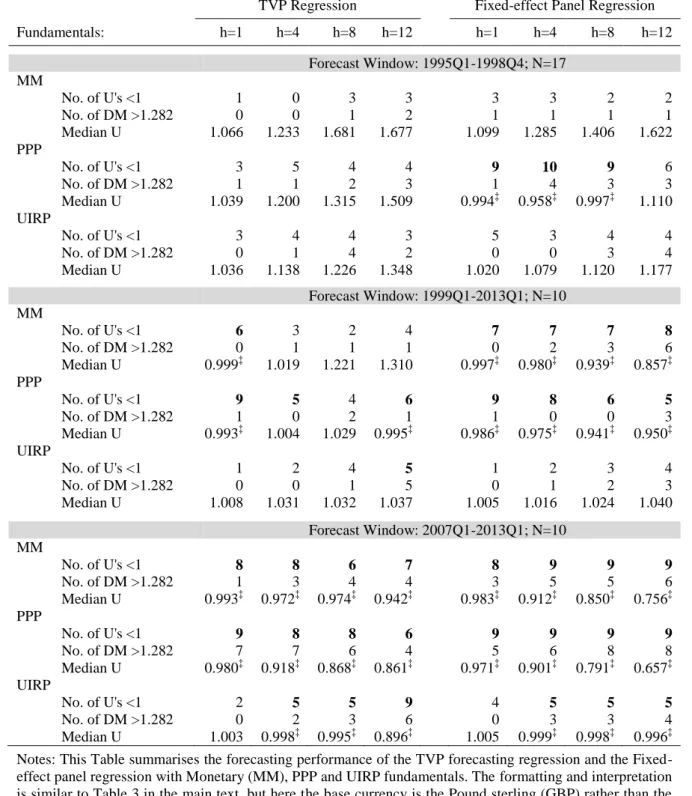
Table 3 illustrates the overall performance of the TVP and the FE panel forecasting

regressions with classic predictors: the MM, PPP and UIRP.

At a glance, regressions

based on PPP perform better than the RW benchmark in all forecast windows and

horizons. That is, the U’s are less than one for over half of the currencies in all forecast

windows and nearly all horizons, regardless of the forecasting regression. Note though that

the FE panel regression yields an outstanding performance in the first forecast window. In

this window, the values of the Median U are substantially below one, and the regression

outperforms the RW for a minimum of 14 out of 17, and as many as 15 exchange rates. By

contrast and in the same window, the TVP forecasting regression does well for a minimum

of nine exchange rates, and a maximum of 11.

Regressions conditioned on fundamentals from the MM fail to improve upon the

benchmark for at least half of the currencies in most windows and horizons. For instance,

while the FE panel regression outperforms the RW for over 14 out of 17 exchanges rates in

the first forecast window and all horizons, in the remaining windows it fails completely.

Likewise, the TVP regression performs relatively well for over half of the currencies

across forecast horizons mainly in the first window. In the other forecast windows it barely

outperforms the RW for at least half of the currencies, except in the last window, at h=8.

Finally, regressions based on UIRP improve upon the RW only for long-horizon

forecasts and often with the TVP forecasting approach. In fact, at h=8 and h=12, the TVP

regression based on UIRP yields a median U below one in the first and last windows.

Consistent with this, the number of U’s less than one reach as many as 10 out of 17 in first

window and five out of 10 in the last window. By contrast, for the FE panel regression, the

Median U is below one in most forecast windows only at h=8. At this forecast horizon, it

out-forecasts the RW for 11 out of 17 exchanges in the first window and five out of 10 in

the last forecast window. We also note that in cases where the RMSFE of the TVP or FE

panel model is lower than that of the RW, the differences in the RMSFE are statistically

significant for long-horizon but not for short-horizon forecasts.

Our results are not unusual in the exchange rate literature. For instance, Rossi

(2013) also reports a poor performance of FE panel models based on the MM at any

horizon. Engel et al. (2008) find improvement over the RW with PPP implied

fundamentals at short and most significantly at long-horizon. Cheung et al. (2005) find

22

Table 3. Forecast Evaluation: Monetary Model, PPP and UIRP

TVP Regression Fixed-effect Panel Regression

Fundamentals: h=1 h=4 h=8 h=12 h=1 h=4 h=8 h=12 Forecast Window: 1995Q1-1998Q4; N=17 MM No. of U's <1 11 13 14 13 14 15 15 14 No. of DM >1.282 5 7 10 11 4 9 12 11 Median U 0.974‡ 0.923‡ 0.703‡ 0.646‡ 0.956‡ 0.785‡ 0.552‡ 0.623‡ PPP No. of U's <1 9 10 11 9 14 15 15 14 No. of DM >1.282 3 7 7 5 9 12 12 11 Median U 0.998‡ 0.935‡ 0.978‡ 0.977‡ 0.974‡ 0.866‡ 0.717‡ 0.759‡ UIRP No. of U's <1 5 10 9 10 10 11 11 11 No. of DM >1.282 1 2 5 8 1 5 10 11 Median U 1.007 0.981‡ 0.985‡ 0.986‡ 0.979‡ 0.969‡ 0.856‡ 0.888‡ Forecast Window: 1999Q1-2013Q1; N=10 MM No. of U's <1 1 1 1 1 1 1 1 1 No. of DM >1.282 0 0 0 0 0 0 1 1 Median U 1.019 1.087 1.216 1.359 1.021 1.100 1.303 1.633 PPP No. of U's <1 8 7 7 7 8 8 7 5 No. of DM >1.282 1 0 2 4 1 2 3 3 Median U 0.994‡ 0.971‡ 0.932‡ 0.857‡ 0.994‡ 0.985‡ 0.972‡ 0.955‡ UIRP No. of U's <1 1 1 3 3 2 2 2 2 No. of DM >1.282 0 0 1 2 0 1 1 1 Median U 1.008 1.030 1.096 1.204 1.009 1.037 1.070 1.137 Forecast Window: 2007Q1-2013Q1; N=10 MM No. of U's <1 2 2 6 4 2 3 4 3 No. of DM >1.282 0 1 2 1 0 0 0 0 Median U 1.012 1.045 0.972‡ 1.021 1.007 1.015 1.057 1.301 PPP No. of U's <1 8 8 7 3 7 8 6 4 No. of DM >1.282 2 4 5 3 3 4 4 4 Median U 0.989‡ 0.924‡ 0.845‡ 1.029 0.991‡ 0.931‡ 0.948‡ 1.260 UIRP No. of U's <1 2 4 5 5 3 4 5 4 No. of DM >1.282 0 0 2 4 0 0 3 2 Median U 1.007 1.009 0.991‡ 0.944‡ 1.012 1.016 0.990‡ 1.026 Notes: This Table summarises the forecasting performance of the TVP forecasting regression and the Fixed-effect panel regression with Monetary (MM), PPP and UIRP fundamentals. See Table 1 for details about the form of the forecasting regressions and how fundamentals are computed or estimated. The benchmark model for both forecasting regressions is the driftless Random Walk (RW). For each regression, set of fundamentals, forecast window and quarterly horizon (h), the “No. of U's < 1” (number of U-statistics less than one), provides the number of currencies for which the model improves upon the RW, since it indicates cases where the RMSFE of the fundamental-based regression is lower than that of the RW. When the U’s are less than one for at least half of the currencies in the forecast window, marked in bold, then on average, the fundamental-based regression outperforms the benchmark in that window. The “No. of DM > 1.282” (number of DM statistics greater than 1.282) shows cases of rejections of the null hypothesis under the Diebold and Mariano (1995) test of equal forecast accuracy at 10% level of significance. The higher the No. of DM > 1.282, the better the average accuracy of the forecasts of the fundamental-based regression relative to the benchmark is. The “Median U” indicates the middle value of the U-statistic across the sample of N currencies for each forecast window and horizon. When “Median U” is less than or equal to one - marked with the symbol “‡”, and U’s are less than one for at least half of the currencies in the window, this is also consistent with a better average forecasting performance of the fundamental-based regression relative to the benchmark.