SOEPL 2009 – An Estimated Dynamic Stochastic General Equilibrium Model for Policy Analysis And Forecasting

(1)

No. 83

SOE

PL 2009

– An Estimated

Dynamic Stochastic General

Equilibrium Model for Policy

Analysis And Forecasting

Grzegorz Grabek

Bohdan Kłos

Grzegorz Koloch

(2)

Design: Oliwka s.c. Layout and print: NBP Printshop Published by:

National Bank of Poland

Education and Publishing Department 00-919 Warszawa, 11/21 Świętokrzyska Street phone: +48 22 653 23 35, fax +48 22 653 13 21 © Copyright by the National Bank of Poland, 2011 http://www.nbp.pl

GRZEGORZGRABEK, BOHDANKŁOS, GRZEGORZKOLOCH, SOEPL−2009— An Estimated Dynamic

Stochastic General Equilibrium Model for Policy Analysis and Forecasting , Bureau of Applied Research, Economic Institute, National Bank of Poland, Warsaw, 2010

(Document compilation: 860.14.2.2011)

Kontakt:

B

[email protected]

T

(0 48 22) 653 15 87

B

[email protected]

T

(0 48 22) 585 41 08

B

[email protected]

T

(0 48 22) 653 21 79

The paper presents the personal opinions of the authors and does not necessarily reflect the official position of the institution with the authors cooperate (have cooperated) or to which they are (or have been) affiliated.

An earlier version of the paper has been published in polish under the title:SOEPL−2009_{— Model DSGE}

małej otwartej gospodarki estymowany na danych polskich. Specyfikacja, oceny parametrów, zastosowania,

Materiały i Studia NBP, 2010.

Typesetting LA_{TEX (TEX, format: LaTeX2e, ver. 2009}_/₀₉_/_{24), pdfTEX, ver. 1.40.11 (MikTEX 2.9)}

LATEX 2

, pdfTEX, BIBTEX (etc.) implementations, fonts, packages of macros and the utilities available in the

MikTEX collection have been used. Detailed information about the licence conditions, software copyrights, legal protection of the stored collection, legally protected trademarks (etc.) are provided on the Internet Web pages of the MikTEX http://www.miktex.org and on the site of TEX system at http://www.ctan.org.

Kontakt:

B

[email protected]

T

(0 48 22) 653 15 87

B

[email protected]

T

(0 48 22) 585 41 08

B

[email protected]

T

(0 48 22) 653 21 79

The paper presents the personal opinions of the authors and does not necessarily reflect the official position of the institution with the authors cooperate (have cooperated) or to which they are (or have been) affiliated.

An earlier version of the paper has been published in polish under the title:SOEPL−2009_{— Model DSGE}

małej otwartej gospodarki estymowany na danych polskich. Specyfikacja, oceny parametrów, zastosowania,

Materiały i Studia NBP, 2010.

Typesetting LA_{TEX (TEX, format: LaTeX2e, ver. 2009}_/₀₉_/_{24), pdfTEX, ver. 1.40.11 (MikTEX 2.9)}

LATEX 2

, pdfTEX, BIBTEX (etc.) implementations, fonts, packages of macros and the utilities available in the

MikTEX collection have been used. Detailed information about the licence conditions, software copyrights, legal protection of the stored collection, legally protected trademarks (etc.) are provided on the Internet Web pages of the MikTEX http://www.miktex.org and on the site of TEX system at http://www.ctan.org.

GrzeGorz Grabek, bohdan kłos, GrzeGorz koloch, SOEPL—2009 — An Estimated Dynamic

Stochastic General Equilibrium Model for Policy Analysis and Forecasting, Bureau of Applied Research, Economic Institute, National Bank of Poland, Warsaw, 2010

(3)

II Specification of DSGE

SOE

PL−2009

model

47

3 SOEPL−2009 _{— general outline} ₄₈ 3.1 SOEEuro_{model — prototype of}_SOEPL_{family models . . . .} ₄₈

3.2 Family ofSOEPLmodels,SOEPL−2009_{version . . . .} ₅₀

3.3 Basic features ofSOEPL−2009_{model . . . 51}

4 Decision-making problems, equilibrium conditions, macroeconomic balance of the model 56 4.1 Growth . . . 56

4.2 Foreign economy . . . 57

4.3 Producers . . . 57

4.3.1 Aggregators . . . 58

4.3.2 Domestic intermediate goods firms . . . 59

4.3.3 Importers . . . 61

4.3.4 Exporters . . . 61

4.4 Households . . . 63

4.5 Behaviour of other agents . . . 68

4.5.1 Central bank . . . 69

4.5.2 Government . . . 70

4.6 Macroeconomic balance conditions . . . 71

4.6.1 Profits in economy . . . 72

4.6.2 Income and expenditures of households . . . 73

4.6.3 State budget . . . 74

4.6.4 Monetary balance . . . 74

4.6.5 Balance of payment . . . 75

4.6.6 The aggregate resource constraint . . . 77

III Results of estimation and characteristic features of the DSGE

SOE

PL−2009

model

78

5 Forms of model, data, SVAR models 79 5.1 Forms of model . . . 79

5.2 Observable variables, data . . . 80

5.3 SVAR models . . . 82

5.3.1 Fiscal SVAR . . . 82

5.3.2 World’s economy SVAR . . . 83

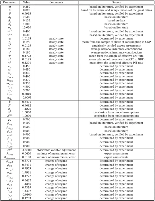
6 Assessment of parameters — calibration, optimisation, steady state 85 6.1 Calibration of parameters . . . 86

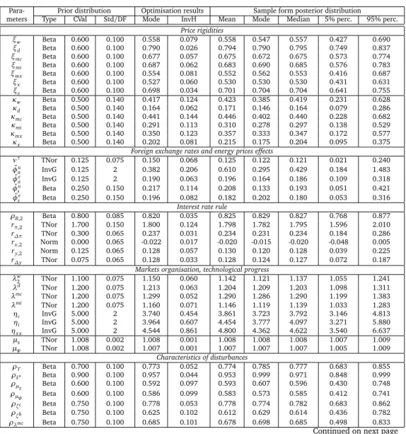
6.2 Prior distributions and results of estimation . . . 87

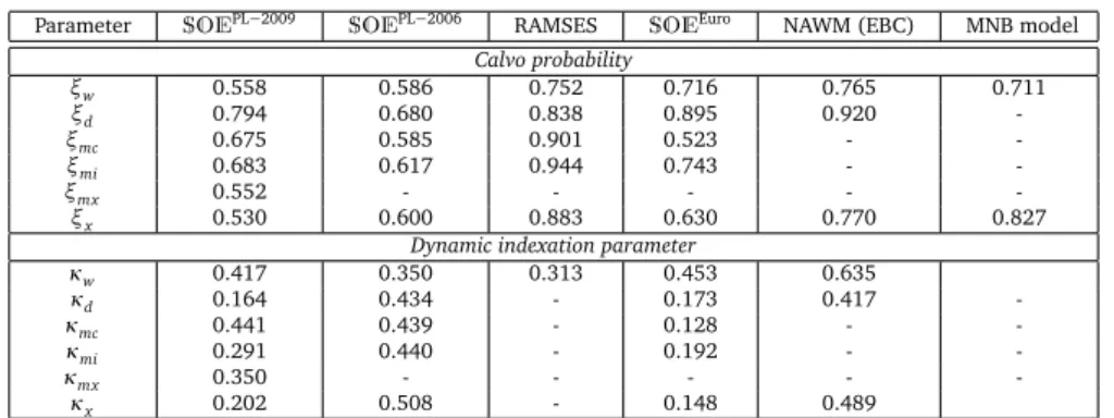
6.3 Assessment of parameters — conclusions . . . 90

6.3.1 Steady state . . . 90

6.3.2 Structural changes . . . 92

(5)

7 Variance decompositions, impulse response functions and estimation of

distur-bances 95

7.1 Variance decompositions . . . 95

7.1.1 Regime I . . . 96

7.1.2 Regime II . . . 97

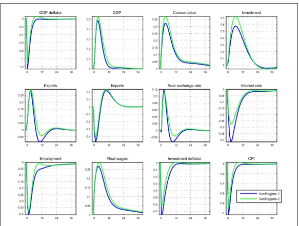
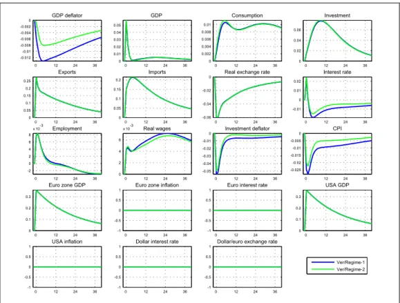
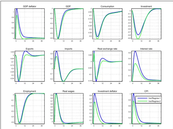
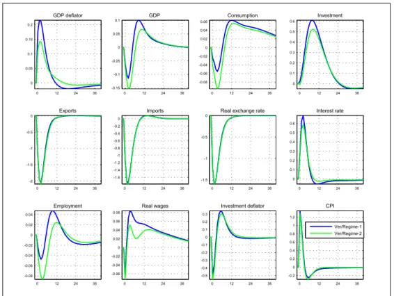
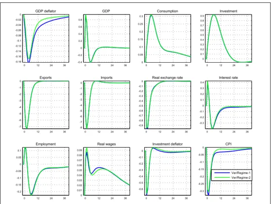
7.2 Impulse response functions . . . 103

7.3 Smoothing — estimation of structural disturbances . . . 118

8 Historical decompositions and forecasts 121 8.1 Historical decompositions . . . 121

8.2 Forecasting technique . . . 122

8.3 Ex-post forecasting accuracy of theSOEPL−2009_{model . . . 126}

8.3.1 One-dimensional measures of forecasting quality . . . 127

8.3.2 Multidimensional measures of forecasting accuracy . . . 128

8.3.3 Rolling forecasts . . . 129

Final comments

132

IV Appendix

134

A List of equations, list of variables 135 Forms of the model . . . 135

List of model variables . . . 136

List of equations of the structural form of the model . . . 139

Steady state solution . . . 144

B Global economy SVAR model 148 SVAR model identification . . . 148

Results of estimation of the SVAR model . . . 148

C Convergence to the steady state 150

D Analysis of forecasts accuracy 151

Bibliogrphy

158

(6)

Introduction

The paper documents the effects of work on the dynamic stochastic general equilibrium (DSGE)

SOEPL _{model that has been carried out in the recent years at the National Bank of Poland,}

initially at the Bureau of Macroeconomic Research and lately at the Bureau of Applied Research of the Economic Institute. In 2009, a team consisting of the authors of this paper developed a new

version of the model, calledSOEPL−2009 _{which in 2010 is to be used to obtain routine mid-term}

forecasts of the inflation processes and the economic trends, supporting and supplementing the traditional structural macroeconometric model and experts’ forecasts applied so far.

In the recent years many researchers have engaged in the work over a class of estimated macroeconomic models (of the business cycle) integrating the effects of at least three important lines of economic and econometric research:

• methods of macroeconomic modelling (gradual departure from the traditional structural

models towards models resistant to Lucas’ and Sims’ critique, strongly motivated with microeconomics);

• micro- and macroeconomic theories (monetary policy issues, with emphasis on the

con-sequence of imperfect competition, the role of nominal and real rigidities, as well as anticipating and optimising behaviours of agents in an uncertain environment, with a strong shift of point of view towards general equilibrium);

• estimation techniques (reduction in parameters calibration, shift from classical techniques

to Bayesian techniques with Bayesian-specific risk quantification as well as systematic and controlled introduction of experts’ knowledge, improvement of projections accuracy). Merger of the three trends has brought about a class of models — DSGE models — with high analytical and developmental potential. The very potential of the models of this class seems to

be the most important reason for the interest of central banks in that area1_{, research that may}

be directly translated into the practice of monetary policy.

1_{Attention is being drawn to the fact that in the general case the DSGE models do not have to be based on the new}

Keynesian perspective of economy and do not have to be estimated with the use of Bayesian techniques.

(7)

Along with the development of numerical, econometric methods and the theory of economics, a number of central banks supplement or even replace the traditional structural macroeconometric models, whose forecasting applications are enhanced with experts’ knowledge, with estimated DSGE models, namely models which attempt to translate the economic processes in a more explicit and systematic manner, whereby experts’ knowledge is introduced through Bayesian

methods2_{. It happens although no formal reasons exist for which the ex post verified accuracy of}

forecasts within the DSGE models should be higher than that of classical models3_{. DSGE models}

give, however, a chance of structural (internally consistent and microfounded) explanations of the reasons for the recently observed phenomena and their consequences for the future. DSGE models present a different image of economic processes than classical macroeconometric models — they capture the world from the perspective of structural disturbances. These disturbances set the economy in motion and economic agents respond to them in an optimal way, which eliminates the consequences of the disturbances, i.e. restores the economy to equilibrium. The analytical knowledge and experience gathered in contact with the traditional structural models rather interferes with than helps interpret the results of DSGE models. In econometric categories, the results of DSGE models are, nevertheless, at least partially compliant with that which may be achieved with VAR and SVAR models, thus, it is hard to speak about revolution here. Following the events of 2008–2009 (global financial crisis), while searching for the reasons for the problems’ occurrence, the usefulness of formalised tools constructed on a uniform, internally coherent (but also restrictive) paradigm for macroeconomic policy tends to be questioned. The reasons for the global economy problems are searched for in models oversimplifying perception of the world and burdening the decisions regarding economic policy. We have noticed that the critique refers to a larger extent to the models as such (i.e. tools) and less to the practice of applying them (i.e. the user). Therefore, we consider that conclusions from a deeper analysis of the sources of 2008–2009 crisis, verification of the directions of economic research and methods of the research, which is likely to be held, as well as the analysis of the current policy less influenced by its rationalisation shall confirm the legitimacy of building and applying models, particularly DSGE class models. The issue of applications using the strong sides of the models remains, however, open. In our opinion, the best we can do is to try to use our model, gather and exchange experience, develop new procedures and thoroughly verify the results.

The model whose details we shall present further herein derives from the structure developed at

Riksbank — DSGE model for the euro area4_{see Adolfson et al. (2005b). The euro area DSGE}

model, know-how, methods of estimation and applications received within the technical support of Riksbank enabled us to start several experiments, build different versions of DSGE model

(a family ofSOEPLmodels) and develop our own procedures of the model application. Some

of the experiments have been described in separate papers, e.g. Grabek et al. (2007), Grabek

2_{For complete image, we wish to add that there are also arguments against the engagement of central banks in}

constructing DSGE models, see e.g. Orphanides (2007).

3_{The issue of correct measuring of accuracy of forecasts, in which the contribution of experts’ knowledge is}

considerable but non-formalised or systematic, has been omitted here. In such a situation it is hard to assess whether it is the model that failed or the expert. Generally, it may be argued whether the forecasting applications of DSGE models expose the strongest sides of this class of models.

4_{The euro zone model by Riksbank develops the ideas mentioned among others by Christiano et al. (2001, 2003,}

(8)

and Kłos (2009), Grabek and Utzig-Lenarczyk (2009). The alternative we present in this paper summarizes some of the gathered experience.

We pass the DSGESOEPL−2009_{model for use, with a view to considering and analysing other}

interpretation and understanding of economic processes than that proposed by the traditional models. Additionally, systematic work with the model (preparing forecasts and analyses of their accuracy, simulation experiments and analytical works) may reveal issues and problems that will have to be solved. Resulting knowledge shall enable the preparation of a more thorough future modification of the model, taking into account the effects of the parallel research and the conclusions arrived at during use.

This paper consists of three basic parts. In the first part — relatively independent of the other parts — we have made an attempt to outline the development of the methods of macroeconomic (macroeconometric) modelling and the economic thought related to monetary policy, which brought about the creation of dynamic stochastic general equilibrium models, pushing aside other classes of models — at least in the academic world. The considerations are illustrated with simple models of real business cycles (RBC) and DSGE model based on new Keynesian paradigm. The second chapter of the first part focuses on the technical aspects of construction, estimation and application of DSGE models, drawing attention to mathematical, statistical and numerical instruments. Although it presents only the keynotes, outlines and ideas, the formalisation and precision of presentation required in that case makes the fragment of the paper slightly hermetic — a reader less interested in the techniques may omit that chapter.

The further parts of the paper refer to specification, results of estimations and properties of the

DSGESOEPL−2009_{model. We present, therefore, a general non-technical outline of the basic}

features of the model, illustrating at the same time the correlations with other DSGE models (Chapter 3). The next chapter defines decision-making problems of the optimising agents, their equilibrium conditions as well as characteristics of behaviours of the non- optimising agents. The description of the model specification is completed with balance conditions on a macro scale.

TheSOEPL−2009_{model has been estimated with the use of Bayesian techniques. Identically as in}

all estimated DSGE models we are aware of, the Bayesian estimation refers solely to some of the parameters (the rest of the parameters have been calibrated). Although due to the application of the Bayesian techniques, the number of calibrated parameters has been clearly reduced, being aware of the consequences of faulty calibration we conducted a sort of sensitivity analysis (examination of the influence of changes in the calibration of parameters on the characteristics

of the model). The presentedSOEPL−2009_{version takes into account the conclusions we arrived}

at based on the analysis. For the purposes of this paper and the first forecast experiments we use only point estimates of the parameters reflecting the modal value of posterior distribution, in other words our reasoning omits — hopefully temporarily — the issue of uncertainty of the parameters. The results of the estimation of parameters and assumptions made at the subsequent stages of the work (calibrated values, characteristics of prior distributions) have been presented in Chapter 6.

A synthetic image of the model characteristics has been presented in Chapters 7–8, which describes the responses of observable variables to structural disturbances taken into account in the model (i.e. impulse response functions), variances decompositions (formally — forecast

(9)

error decomposition), thanks to which the structure (relative role) of the impact of shocks on the observable variables may be assessed, estimation (identification) of structural disturbances in the sample, examples of historical decompositions (counterfactual experiments) and information about the ex post accuracy of forecasts — this is, thus, a typical set of information allowing understanding the consequences of the assumptions made at the stage of constructing decision-making problems (model specification) and choice of parameters.

The Appendix presents structural form equations, equations used to determine value at a steady

(10)

Genesis and anatomy of dynamic

stochastic general equilibrium

models

(11)

1

Chapter 1

Genesis and anatomy of dynamic

stochastic general equilibrium

models

The development of economic models for the purpose of monetary policy analysis has been one of the most exploited research programs within macroeconomics in the last two decades. A lot of effort has been paid to make attempts to understand the correlations between monetary policy, inflation and business cycle. The research is deemed to produce a sort of consensus as to the specification of the key elements of a model of economy, within which modern macroeconomic analysis is being carried out, mainly in the aspects important for the monetary policy applied by central banks. The specification has been named a new Keynesian model. The new Keynesian model is a dynamic, stochastic model of general equilibrium and, thus, a model deriving from neo-classical trend. The basis for its architecture is a model of real business cycle, on which

Keynesian elements in the form of real and_/or nominal frictions1_{are imposed. Such originating}

trend of macroeconomic analysis is called a new neoclassical synthesis, see Goodfriend and King (1997).

1.1 Methods of the Cowles Commission

In the 1940s and 1950s government institutions of the most important economies started to collect in a systematic way national statistics regarding economic activity. The economists gained material which helped them specify quantitative models of national economy and analyze them in empirical tests. Early works over the econometric models of national economies complied with

1_{E.g.: monopolistic competition, frictions in the process of adjusting prices, wages, frictions in the financial market.}

11

1

Genesis and anatomy of dynamic stochastic

general equilibrium models

(12)

1

the paradigms developed during the works carried out by the Cowles Commission. Empirical

macroeconomic analysis was at that time carried out with often large2_{, dynamic, most often}

linear, multi-equation econometric models. Their specification was based mainly on statistical

tests3_{, while the role of economic theory was limited to preparing a list of regressors to be taken}

into account in the particular equations. The choice of variables was based mainly on Keynesian IS-LM type models, i.e. on theories which ignored both the supply side of economy and changes in relative prices. The models were called ”structural”, as they enabled the consideration of, among other things, feedback nature relationships between variables. Such relations and the resulting problem of simultaneity or interrelation, important for model estimation techniques, were the focus of interest of macroeconometrics and the theory of estimation at that time. Therefore, it is considered that econometrics practiced in the spirit of the Cowles Commission emphasised the structural aspects. Nevertheless, according to today’s understanding of structurality in macroeconomics, it may be concluded that structurality, or practically its absence primarily accounted for the failure of this trend of modelling. Although model equations were aimed at presenting the dynamics, which reflects the decisions made by economic agents, forms of equations assumed ad hoc failed to comply with any mechanism of individual choice. Dynamics of each of the variables would be modelled with a single equation. Groups of variables formed the blocks of a model and each block was researched by a separate group of experts. The resultant equations were later on combined in a complete model of economy, additionally taking into account the interactions occurring among the variables within the different blocks. The constructed models allowed, seemingly, correct quantification of the consequences of controlling variables that depended on the persons making decisions with regard to economic policy. They were, however, too large to arrive at a general image of the mechanism according to which the propagation of shocks in an economic system took place. It was also hard to research the mechanism of system response to a change in control of economic policy in a longer time perspective. According to the philosophy of the Keynesian trend, the emphasis was put on short-term analysis of economic aggregates dynamics. The economy was out of (partial) equilibrium for a short period and model simulations answered the question of how to effectively bring the economy to equilibrium, i.e. how to stabilise it. Thus, macroeconometrics dealt mainly with the analysis of variables dynamics in a short time with the use of partial equilibrium model. An example of a model within the discussed class is provided in Klein and Goldberger (1955).

1.1.1 Problems with identification

In the terminology derived from the paper of Spanos (1990), the reasons for failure of the originators of models maintained in the tradition of the Cowles Commission as regards the application of the models to economic policy analysis may be divided into two groups. These are problems with structural identification and problems with statistical identification.

As mentioned by Hendry (1976) or Qin (1993), in the period of works of the Cowles Commission and the later development of multi-equation models maintained in this tradition,

economet-2_{Consisting of several hundred or, sometimes, even several thousand equations.} 3_{A statistical identification of model is often being mentioned.}

(13)

1

rics focused to a large extent on the theory of estimation4_{, and a smaller emphasis was put}

on the assessment of the quality of models by virtue of diagnosis of statistical specification errors. Structural identification was a priority and as a result, often proved ex post, the models maintained in this convention were not able to sufficiently accurately replicate the statistical properties of the processes the dynamics of which they were supposed to represent. Although the Cowles Commission was putting emphasis on structural identification of the model, the developed methods are considered, from the perspective of the present day, to be unsatisfactory. Problems with structural identification were more fundamental. They are presented, among others, in two papers from the 1970s and 1980s: Lucas (1976) and Sims (1980). Lucas (1976) criticises the status of exogeneity of variables — the controls of economic policy. He points out that the model of structural identification proposed by the Cowles Commission does not explicitly take into account the expectations of economic agents. Therefore, the parameters of

the mode5_{, which were deemed to be structural}6_{, are actually a mixture of structural parameters}

and parameters related to the expectations of economic agents and, thus, may not be considered to be fixed for various economic policy regimes. The estimations of parameters within a model estimated on data originating from a specific economic policy regime shall no longer be valid if the policy regime changes. Therefore, a model estimated within one regime may not be extrapolated outside of the regime and, in consequence, may not be applied to analyse the consequences of a change in the regime. Due to instability of parameters, the traditional structural macro-models, according to Lucas, are worthless for simulation of the effects of changes in economic policy, which is exactly the purpose for which they were created. Sims (1980) only supports the comments by Lucas claiming that no variable may be deemed exogenous in the world of economic agents that anticipate future events (forward-looking agents) and whose behaviour is based on intertemporal optimisation. As a result of endogenous economic policy macroeconomic variables correlate with variables — the controls of policy. By assuming erroneously that the policy is exogenous, the endogeneity may be falsely interpreted as a causal relation, and may seem to identify the channel of policy’s impact on economy.

Finally, the stagflation of the 1970s and the related failures of economic policy based on the traditional macroeconometric models disqualified, in the academic opinion, the approach of the Cowles Commission. Pesaran and Smith (1995) conclude that the models represented neither the data, nor the theory, and therefore were ineffective for practical purposes of forecasting and policy.

1.2 LSE and VAR models

Problems with statistical and structural identification of traditional multi-equation econometric models brought about the development of several trends out of which two had the largest impact

4_{Important in the works of the Commission and later works were mainly the issues regarding simultaneity, i.e.}

interrelation of the modelled phenomena.

5_{This specifically refers to the so called reduced form of the model.}

6_{Parameters are deemed to be structural or deep if their value does not change under the impact of a change in the}

(14)

1

on the practice of macroeconometrics: the so-called LSE method (London School of Economics), see Hendry (1995), and SCVAR method (Structural Cointegrated Vector Autoregression), i.e. structural vector autoregression for cointegrated variables, see Lütkepohl (2008), which currently — next to the DSGE model — is the basic tool of macroeconomic analysis.

1.2.1 LSE methodology

There may be numerous possible sources of errors in statistical identification of a model. The errors include, but are not limited to, omitting important variables, erroneous dynamic structure or illegitimate restrictions regarding exogeneity imposed on the variables. The LSE approach is an attempt to overcome the problems with statistical identification. It is based on the so-called reduction principle. An econometric model is understood as a simplified representation of an unknown and unobservable stochastic process, which generated the researched economic observations. It originates from a dynamic model of possibly general specification in a given class of models, so as to cover possibly many various processes. Further on, the model is reduced sequentially to the final form. The reduction step entails the elimination of a variable or a group of variables from the model and is made with the use of statistical tests. For the resulting representation of a process that generates data to be complete, loss of information by virtue of reduction must be insignificant from the point of view of the modelled process. A completeness of the model is confirmed by the statistical properties of the residuals vector. Any deviations from the Gaussian white noise certify that specification is faulty. Thus, the LSE approach emphasises the correct statistical identification of a model but is not an attempt to solve problems related to structural identification.

1.2.2 VAR methodology

Similar problems are reflected in the approach based on the analysis of time series with the use of non-structural models of vector autoregression (VAR). Non-structural VAR models, or VAR models in reduced form, are in fact the generalisation of the LSE approach to vector time series. They are models expressing endogenous variables by their lagged values. A VAR model of order

K_≥1 has the following form:

y_t₌ K k=1

A_ky_t₋_k₊e_t, or y_t₌Ay_t₋₁₊e_t, (1.1)

where y_t is a vector of endogenous variables in t period, A_k matrices for k₌1, 2, ..., K are

autoregressive matrices. Another representation is called a cumulative representation andA

matrix is an autoregressive companion matrix. The e_t process covers shocks controlling the

dynamics of endogenous variables. The e_t shocks control the dynamics of endogenous variables

such that the variables may be presented as a function of the history of shocks. This is the

(15)

1

y_t₌At_y 0+ t−1 k=0 Ak_e t−k, (1.2)

where y₀is the initial value of the process(yt), or — assuming infinite history of the process of

endogenous variables: y_t ₌ ∞ k=0 Ak_e t−k. (1.3)

The basic purpose of the macroeconomic analysis carried out in accordance with the concept of a shock impacting the system of endogenous variables as a source of their dynamics is to identify shocks of structural nature, i.e. independent shocks with explicit and cohesive economic

interpretation. The e_t shocks may not, however, be structurally interpreted as they do not need

to be independent, and generally are not, which should be expected from shocks of structural

nature. The e_t shocks have the nature of errors or regression residuals (forecast errors) and

may form linear combinations of the actual structural shocks which determine the dynamics

of endogenous variables. It may, then, generally happen that e_t ₌Bεt, whereεt are structural

shocks, i.e. independent ones. In particular it is assumed that the covariance matrix ofεt shocks

is the identity matrix, i.e.(εt) =I. This leads to the approach giving structural interpretation

to VAR models. The approach is called structural vector autoregression, shortly SVAR (from structural VAR). Next to the advantages of the LSE approach in the form of representation of a process generating the dynamics of endogenous variables through a model of rich dynamic structure, namely VAR, the SVAR methodology makes it possible to provide shocks with structural interpretation.

The SVAR methodology has been developed not only for stationary processes on which the approach based on the Cowles Commission paradigms must rely, but may be easily generalised to non-stationary cointegrated processes. Such approach is called structural cointegrated vector autoregression method, shortly SCVAR, or more often — structural vector error correction model, shortly SVECM.

SVAR and SVECM models attempt to solve problems regarding statistical identification and some of the problems regarding structural identification, which were identified in the classical multi-equation models. These advantages explain the popularity of VAR class models in empirical macroeconomics. In order to emphasise that there have been proposed at least partial solutions not only for statistical identification problems but also for structural identification, modern macroeconomic analysis is often referred to as structural macroeconometrics. Despite the aforementioned advantages, VAR methods are not free of drawbacks. Mainly, VAR models specification lacks any theoretical basis. The relations between the variables are of clearly statistical nature and even in the case of structural models they may not be referred to any economic mechanism on which the modelled process is founded. Thus, a VAR model lacks a theoretical framework, and upon assessment it may bring about, and in practice often brings, non-intuitive implications in the form of responses to shocks that may hardly be rationalised and

(16)

1

non-cohesive forecasts. Due to the foregoing disadvantages, macroeconomic analysis, particularly at central banks, more and more often refers to models having theoretical foundations, such as DSGE models.

DSGE models - through economic theory underlying their specification — constitute another step forward to solve the problems with structural identification. The step is taken at the cost of statistical quality of the model, however not so significant because the DSGE models, and more specifically their approximate solutions, are directly related to VAR class models. Specifically, the so-called reduced form of DSGE model, namely the form which sets dynamics of endogenous variables around the equilibrium, is a VAR model. It may be considered as a VAR model on

the parameters of which, i.e. on elements of matricesA and B, a set of restrictions has been

imposed. The restrictions originate in the theory of economics underlying the specification of a DSGE model. They limit the dynamic structure of the model, yet ensure its internal cohesion and guarantee structural nature of the identified shocks. The DSGE model specification founded on the theory of economics ensures that restrictions imposed on the dynamic structure of its reduced form derive from the optimal decision-making rules of rational economic agents operating in an internally cohesive economic reality. The methodologies of DSGE models are, therefore, at least theoretically, an answer to the problems related to structural identification. They also, to a major extent, reply to the problems related to statistical identification, as the solution of a DSGE model is a VAR class model. In that scope a DSGE model provides, nevertheless, only partial solutions, as the structural nature of its specification imposes strong restrictions on the dynamic structure of the reduced form. Thus, a DSGE model expresses a trade-off between the proper statistical and structural identification of macroeconomic processes.

1.3 Methodology of modern macroeconomics

The views with regard to the method of analysing the dynamics of economic aggregates have significantly changed over the last 30 years. The evolution followed from models specified in the tradition of the Cowles Commission, through VAR class models, to dynamic stochastic general equilibrium models based on the theory of economics.

Modern macroeconomics attempts to explain the dynamics of economic aggregates with the use of models based on the so-called microfoundations. Hence, as opposed to traditional Keynesian models or multi-equation macroeconometric models where the forms of interrelations between economic variables were assumed ad hoc, the mechanisms shaping the decision-making rules of economic agents are explicitly modelled. Most often four types of agents are distinguished. They are households, firms as well as government and central bank. Whereas the decision-making rules of households reflect the process of optimisation of welfare, i.e. a discounted stream of the expected utility, those of firms result from maximisation of the expected profit. Optimisation takes place in a stochastic economic environment and in the case of households the structure of their preferences — the so-called utility function — is also set. The decisions of agents are, thus, always optimal a priori, i.e. the best of possible taking into account the available information. Usually, they refer to three types of economic categories: products and services, work or assets, both physical such as capital and financial such as bonds or money. Households decide about

(17)

1

consumption, i.e. demand for a product, supply of labour and change in the structure of the portfolio of financial assets, the level of investments, the level of use of the available capital, etc.

Firms decide about product supply and demand for labour7_{. The government determines the}

value of public spending, collects taxes, expends transfers and incurs public debt. The central

bank controls the nominal interest rate and/or the supply of money. The decision rules of the

government and the central bank are usually made ad hoc. Beside of the optimisation criterion, the process of making decisions by economic agents takes into account several categories of limiting conditions. These are most often budget constraints, initial conditions, equilibrium conditions and constraints regarding the available technology and information structure in the

economy8_.

A central issue in the theory of dynamic general equilibrium is the intertemporal dimension of the decision-making process. The decisions of agents consist of intertemporal allocation of the available resources. Today’s income may be allocated to future consumption and future income may finance today’s consumption expenditures. Intertemporal substitution of resources is possible by virtue of participation in the market of financial assets, e.g. purchase or sale of bonds. The individual decisions are coordinated by the market, which brings about decentralised allocation of resources.

Formally, economy is described as a dynamic system. It reflects a short-term equilibrium in at least two meanings. Firstly, in each point of time economy reflects a general equilibrium as understood by Walras. It is, thus, assumed that prices always clear the markets. Secondly, economic agents make optimal decisions, i.e. ex post they do not make mistakes in a systematic manner as to the actions undertaken. In that meaning their decisions are called rational. Should it appear ex post that the decisions of the agents are not the best possible to be taken, this is only due to information gap, i.e. due to the fact that after the moment of making the decision an event occurred that could not have been foreseen by the agent, e.g. an unexpected exogenous growth in productivity took place. The agents build expectations as to the future values of economic variables through the operator of conditional expected value. In that sense the mechanism of building expectations by the economic agents is rational. It is, therefore, assumed that agents know the complete model of economy, namely that they know (the real) principles governing the world in which they live and the values of all of its parameters. They are also able, based on the model, to set out optimal decision-making rules for all agents and apply them, which would require in practice the possibility of making a perfect filtration, i.e. a perfect measurement of the value of all of the variables and shocks impacting the economy in any period. That omnipresent transparency and rationality draws critique on the part of alternative paradigms of economic modelling such as multi-agent modelling (agent-based computational economics), see Fagiolo and Roventini (2008).

Even though the economy is — in the above meaning — assumed to remain at all times in short-term equilibrium, in a short period it may be out of long-short-term equilibrium. Long-short-term equilibrium is also called stationary state or steady state. The names are founded on mathematics.

7_{The mentioned division into the decisions of households and firms is conventional, however, characteristic to the}

literature of the subject matter.

(18)

1

Long-term equilibrium is a mathematical concept and refers to the model of economy instead of the economy in itself. There is no direct equivalent in the real world. Economy reflects long-term equilibrium if all of the variables grow from one period to another according to

fixed growth rates9_{. Economy in a steady state may be knocked out from the state. It happens}

because stochastic disturbance, i.e. structural shocks or structural innovations impacts the economy. Examples of structural shocks are technological shocks (increase or drop in total factor productivity), shock of preferences or contractionary monetary policy. If the effects of shocks abate, the economy comes back to long-term equilibrium but not necessarily to its pre-shock state. This shall happen if the effect of shock is permanent. If economy is knocked out of long-term equilibrium by a shock of temporary effect, it shall asymptotically come back to the same equilibrium. As in reality structural shocks happen at any moment, the real economy shall never come to the same steady state. It shall, however, fluctuate in its environment. The steady state path may be interpreted as the path taken by the economy would it not be for the shocks. A model implying the comeback of economy to the steady state upon structural shock occurrence is called a steady-state or stationary model.

Modern macroeconomic analysis decomposes the time series of economic aggregates into two basic components, namely long-term trend and short-term cyclic fluctuations around the trend, i.e. the so-called business cycle. It shall be emphasised that both the trend and the cycle are statistical fiction and have no equivalent in the real world. Both categories are a product of data filtration and their form depends on the chosen method of filtration. DSGE models, as ones deriving from the RBC models family, are used in cycle analysis and due to their construction are not able to answer any question regarding the forming of the trend. This is the subject of the theory of economic growth, which is introduced to DSGE models in an exogenous manner.

1.3.1 Real Business Cycle theory

Since the beginning of 1980s, when the first papers of the type Kydland and Prescott (1982) appeared, the theory of Real Business Cycle (shortly RBC) has gained the status of a leading macroeconomic theory with regard to economic fluctuations analysis — a model that may be called a standard RBC model from today’s perspective, the basic tool of business cycle analysis. The influence of the RBC revolution on understanding short- and medium-term economic fluctuations has two perspectives — both methodical and conceptual.

From the methodological point of view, the theory of Real Business Cycle made the dynamic stochastic general equilibrium model a basic tool for macroeconomic analysis. Ad hoc assumed behavioural equations describing economic aggregates gave way to equations of motion derived from intertemporal solutions of optimisation problems of the economic agents operating in perfectly competitive and friction-less markets. Ad hoc assumptions made with regard to the mechanisms of forming expectations by economic agents gave way to rational expectations. The creators of the RBC trend emphasised as well the importance of quantitative aspects of macroeconomic analysis, which was reflected in the use of the methods of calibration, simulation and validation of RBC models.

(19)

1

Equally fundamental proved to be the conceptual implications of the RBC theory. Firstly, it appears from the RBC theory that a business cycle presents an effective, i.e. optimal path of economic aggregates. In other words, both expansion and contraction result from optimal reaction of economic agents to exogenous shocks impacting the real sphere of economy, mainly technological shocks. Thus, cyclic fluctuations — including recessions — do not bring about ineffective allocation of resources — they are fully optimal and do not result from market imperfections. The RBC theory implies, therefore, that the stabilisation policy of a government may change resources’ allocation but only to less efficient one. This clearly contradicted the standard Keynesian interpretation of recession as a period in which economic resources are used ineffectively and the end of which may be advanced by stimulation of aggregated demand. The second implication of the RBC theory is the conclusion that the main reason for economic fluctuations are technological shocks, which temporarily improve or deteriorate the total factor productivity in the economy. RBC models try to replicate the fluctuations of products and other economic aggregates, even if the only shock impacting economy is the shock of productivity. Such interpretation of economic fluctuations contradicted the traditional view that changes in productivity contributed to economic growth, which has nothing to do with a business cycle. The third fundamental conceptual implication of the RBC theory is the limited, or practically non-existent, role of monetary factors in economy. A standard RBC model implies the neutrality of money even in a short period. Hence, the dynamics of real variables in economy, such as production, consumption or employment, do not depend on monetary policy. Monetary policy may only affect the nominal values such as the nominal interest rate or nominal supply of money, namely inflation, whose values do not affect the real sphere of economy. The results contradicted the general opinion that monetary policy impacts the real economy in a short run, see Friedman and Schwartz (1963) and Christiano et al. (1998). Even though the RBC theory had a considerable influence on the method of understanding business cycles, particularly in the academia, RBC models — due to the results regarding the neutrality of money — were not accepted by central banks. The central banks continued to focus on classical multi-equation models and more and more often on LSE type approach, particularly on vector autoregression methods.

Due to the growing evidence of contradictions between the Real Business Cycle theory and empirical research, as well as rift between its implications and the practice of economic policy, RBC methods could not be considered satisfactory. On the other hand, RBC methods proposed solutions to problems that discredited the traditional approach based on paradigms developed by the Cowles Commission. RBC models are dynamic stochastic general equilibrium models instead of partial equilibrium models. They have an internally cohesive theoretical structure. Therefore, even though they are calibrated (today, estimated) based on the data that may be generated by non-intuitive statistical artefacts, the results of simulation experiments (e.g. forecasts, shock response analyses) reflect internal cohesion. This is not the case with VAR class models, even the structural ones. The decision-making rules of economic agents in an RBC model are structural, i.e. derived from microfoundations instead o f being assumed ad hoc. The expectations of agents are rational, while anticipation of future events influences their today’s behaviour. RBC models reflect, therefore, the achievements of the revolution of rational expectations. RBC models

(20)

1

parameters, or at least some of them, are deep parameters. Thus, the models are at least partially resistant to Lucas’ and Sims’ critique. In other words, the models allow us to correctly analyse the effects of changes in economic policy regime. All those features indicate that RBC methods well manage the problems of structural identification. Additionally, the reduced form of an RBC

model is a VAR type model10_{, namely a model covering a wide class of stochastic processes.}

This feature shows that problems related to statistical identification are not ignored in the RBC methods.

It is clear that RBC methods could not be simply rejected. Thus, attempts of such modification of the Real Business Cycle theory have been made so that the internally cohesive structure of an RBC model be preserved, their dynamics be related to VAR class models, while the role of money be increased in a short time. The introduction of the elements of new Keynesian economics to the classical RBC model proved to be a solution — such derived model is called a new Keynesian model. We will start with the frictionless monetary model of the economy and then introduce some frictions which render money non-neutral.

1.3.2 Frictionless economy

A standard frictionless monetary model is presented below11_{. Despite a simple structure, it}

presents the most important components of a DSGE model. In the following paragraph the model is extended with Keynesian elements, which leads to the basic form of a new Keynesian DSGE model. A standard DSGE economy consists of a representative household, a representative firm and a central bank. The presentation of the standard DSGE model in this paragraph has been founded on the monograph by Gali (2008).

1.3.3 Representative household

In exchange for nominal wage W_t,a household provides a representative firm in each of the

periodst₌0, 1, 2, ... with a homogenous labour supply12 _Hs

t. The labour market is perfectly

competitive. In exchange, a household receives wage of the worth of H_tW_t. The wage, together

with the savings B_t₋₁in period t₋1, is the income of a household D_t₌H_tW_t₊B_t₋₁, which is

divided between consumption C_t and savings B_t. A household consumes homogenous goods

(products) manufactured by the firm, while the unit price of the product is P_t. Savings are

located in bonds with no risk. A unit price of bonds in period t amounts to Q_t₌₁1

+i_t, where it is

the nominal interest rate determined by the central bank. One bond purchased in period t at

price Q_t is worth in period t₊1 one monetary unit. The expenditures of a household in period t

are, thus, PtCt+QtBt. Household’s welfare is measured with a utility function U(Ct, Ht), while

consumption increases and labour decreases welfare.

10_{The reduced form of a DSGE model is a process of VARMA class, perhaps of infinite order, however, in practice the}

process is approximated with a finite order VAR model.

11_{The presented version of the model abstracts from investments and government sector. Beside those simplifications,}

the model corresponds to the standard specification of an monetary model which builds on the RBC origins. The assumed simplifications are non-significant from the point of view of the presented conclusions.

12_{Subscript s stands for the supply of labour offered by a household. Subscript d shall stand for demand for labour}

reported by a firm. In general equilibrium Hs

t=hdt, therefore, subscripts s or d shall be omitted when it must be emphasised that we mean the labour in general equilibrium.

(21)

1

In period t, a representative household must, then, make a decision as to variables_{C_t, Hs

t, Bt},

such as to maximise utility and by virtue of spending P_tC_t₊Q_tB_tnot to exceed the budget of

the value ofW_tHs

t+Bt−1. Decisions of a household are not, however, one-period problem, i.e.

their consequences are not important only ”here and now”. The decision-making process has a dynamic, multiperiod nature, as today’s decisions affect the value of resources available

tomor-row. A household must, then, decide not only about variables{C_t, Hs

t, Bt}for the determined t

but also for all of the t₌0, 1, 2, ... at the same time. In order to know how to do that, in t₌0

period a household solves the problem of maximisation of the discounted stream of the expected utility: max {C_t,Hs t,t=0,1,2,...}0 ∞ t=0 βtU(Ct, Hst), (1.4)

subject to a sequence of budget constraints:

P_tC_t₊Q_tB_t₌W_tHs

t+Bt−1, (1.5)

wheret is the operator of the conditional expected value. Problem (1.4–1.5) may be solved by

using Lagrange’s functional in the form:

= _∞ t=0 βt[U(Ct, Hts) − ωt(PtCt+QtBt−Bt−1−WtHts)] . (1.6)

First order conditions are as follows:

ωt= ∂U(Ct, Hst) ∂Ct 1 P_t, ωt= − ∂U(Ct, Hst) ∂Hst 1 W_t oraz ωt= β Q_ttωt+1, (1.7)

and for CRRA13_{type utility function, the decision rules of a household are the following:}

C_t₌ _Q t β t{(Ct+1) σc_Π t+1} 1 σ_c , Wt P_t = (Hts)σhC σ_c t . (1.8)

System (1.8) is recursive. The first equation, i.e. consumption’s law of motion, determines the

value of consumption C_t depending on the expected consumption C_t₊₁and inflationΠt+1. The

second equation — labour supply equation — determines, for the assumed real wage value, the supply of labour that needs to be provided by a household in order to generate income

necessary to cover the costs of consumption. The choice of_{C_t, Hs

t, t=0, 1, 2, ...}shall maximise

the expected welfare of the household.

13_{The constant relative risk aversion utility function is defined as:}

U(Ct, Ht) =(

C_t)1−σc₋₁

1− σc −

(Ht)1+σh−1 1− σh .

(22)

1

1.3.4 Representative firm

A representative firm hires labour supplied by a household Hd

t in exchange for nominal wage Wt.

It manufactures a homogenous real product Y_t with the use of production function Y_t₌A_tN_t,

where At is an exogenous process of total factor productivity. The product market is perfectly

competitive. A decision-making variable in the case of a firm is the demand for labour Hd

t, which

— for the assumed technology level — determines the value of the product. In order to determine

the Hd

t value, a firm solves in each period a static problem of profit maximisation:

max Hd t P_tY_t₋W_tHd t , subject to the technological constraint:

Y_t₌A_tHd t,

the solution of which implies equating real wage with marginal productivity of labour: A_t₌Wt

P_t , which is exogenous.

1.3.5 General equilibrium

Upon determination of optimal decision rules of a representative household and a representative firm, market clearing conditions are imposed on all markets, i.e. the economy is assumed to remain in general equilibrium state in every period.

The model in its existing form is linear. Generally, no satisfactory methods exist to solve non-linear DSGE models. Therefore, the equilibrium conditions are superimposed on the simplified,

log-linear form of the model, which for the presented frictionless model reads as follows14_:

c_t₌_tc_t₊₁₋ 1 σc( i_t₋_tπt₊1− ρ), w_t₋p_t _{= σ}_cc_t_{+ σ}_hhs t, w_t₋p_t₌a_t, y_t₌a_t₊hd t, (1.9) where_{ρ = −}lnβ.

In the basic model there are three markets — product market (consumption balancing), labour market and savings (bonds) market. The product market’s clearing condition states that the

14_{Small letters denote in this chapter percentage (logarithmic) deviations from the steady state. Exceptions: real and}

nominal interest rates, which are expressed in absolute values, as well as real marginal costs and monopolistic markup which are expressed in logs. Timeless variables denote steady state values.

(23)

1

whole product supply y_t is subject to consumption:

y_t₌c_t the labour market clears when:

hd

t =hst=ht.

Whereas households trade bonds only between one another, the savings market clears automati-cally:

b_t ₌0.

The condition equating real wage with marginal productivity of labour, after log-linearisation

w_t₋p_t₌a_t, may be read out as the determination of real marginal cost (denoted by mc_t) or —

equally — monopolistic markupλt= −mct, equal to one (zero for the logarithm):

mc_t_{= −λ}_t₌w_t₋p_t₋mpn_t₌0,

where mpn_t₌a_t stands for marginal labour productivity.

1.3.6 Consequences for monetary policy

Based on the conditions (1.9) and the market clearing conditions, there may be determined the

dynamics of real categories of product y_t, employment h_t, real wage w_t₋p_t and real interest

rate rt=it− tπt₊1: c_t₌y_t₌ σh+1 σh+ σc a_t, h_t₌σh σc 1_{− σ}_c σh+ σc a_t, w_t₋p_t₌a_t, r_t_{= ρ +}σc(σh+1) σh+ σc (ρ − 1)at, (1.10)

where technology15_{is controlled with an exogenous stationary process in the form of:}

a_t_{= ρ}a_t₋₁_{+ ε}_t,

whereεt∼N(0,σ)is a structural shock of labour productivity. In a standard RBC model this is

the only structural shock. The last of the equations above, i.e. the real interest rate equation

r_t₌i_t₋_tπ_t₊₁, results from Euler household equation.

It appears then that the dynamics of real variables in a standard frictionless economy model

depends only on the level of technology at16. Therefore, from Fisher equation: rt=it− tπt₊1,

it results that a change in the nominal interest rate is one to one translated into a change in

15_{More precisely, the process of total factor productivity (TFP), here — labour productivity.} 16_{And in the case of real interest rate — on the expected change in technology}

(24)

1

inflation expectations. The equilibrium dynamics of real categories does not depend on the

nominal interest rate i_t, as the interest rate is translated only to nominal category — the expected

inflation. Monetary policy does not affect the decision rules of firms and is neutral for the welfare of households. Consequently, a standard RBC model implies that implementation of monetary policy, requiring high monetary and institutional expenditures, is non-productive.

1.4 New neoclassical synthesis

The conclusion regarding the neutrality of money in a standard frictionless monetary model of the economy was a decisive factor that the models of that class could not raise serious interest at institutions such as central banks, whose practice and understanding of economic categories fluctuations contradicted the implications of Real Business Cycle theory. On the other hand, microfounded models gained the interest of academic communities because — compared to previous macroeconometric models — they made a significant step ahead from the point of view of the method of economic modelling. They appeared particularly attractive due to explicit modelling of the decision-making process of economic agents and specification of the model based on structural parameters — unchanging in the analysis of alternative scenarios of economic policy, including monetary policy applications. Therefore, the normal course of events seems to be the beginning of construction of a new theoretical trend based on a possibly simple case, which would, however, reflect the central elements of the trend. In the case of the trend that originated as an effect of merger of the RBC theory with the elements of new Keynesian economics — the trend that is currently called new neoclassical synthesis — the starting point was the model of general equilibrium of frictionless economy (or distortion-free economy). Neutrality of money and the primacy of technological shocks in the course of the cycle contradicted economic practice and the concept that demand factors and monetary shocks should play more than marginal role in forming the cycle. This leads to many attempts of developing the originally frictionless monetary models towards specifications abiding by the methodical achievements of that trend, however, implying non-neutrality of money in a short run.

In the 1980s and 1990s the analysis covered various microeconomic mechanisms, mainly the so-called distortions or non-effectiveness, the purpose of which was to bring the general equilibrium models closer to economic reality. A number of papers proposed methods to consider nominal rigidities in the dynamic model of general equilibrium. Initially — analogically to new Keynesian literature — emphasis was being put on rigidities in the process of adjusting prices. The proposed models in fact extended the standard frictionless framework to the case of firms operating in the market of monopolistic competition which are not always able to determine markups or, equivalently, prices at the optimal level. The choice of distortions in the process of price or markup determination offered the simplest solution guaranteeing that monetary shocks shall have real effects and shall reflect adequate persistence. In the following paragraph, we present a standard new Keynesian model based on a standard frictionless engine, emphasising the reasons for non-neutrality of money.

(25)

1

1.4.1 Standard new-Keynesian model

Economy consists of a representative household, firms — no longer a representative firm — and central bank. The economic environment in which a representative household is operating is identical as in the standard frictionless monetary model. Hence, that decision-making problem of a representative household, as well as its decision-making functions are the same as in the standard frictionless monetary model. The central bank implements monetary policy applying the monetary policy rule, e.g. Taylor rule. The main difference appears in the sector of firms that possess monopolistic power, so they are no longer price takers. It is assumed that there is a

continuum of firms and each of them is represented by a point on_[0, 1_]17_{interval. They operate}

in the market of imperfect competition, usually monopolistic competition. Thus, firms have monopolistic power and may determine the prices of their products. Each firm manufactures a product different from the products manufactured by other firms (a variety), while the elasticity of substitution between products manufactured by various firms is finite. The products of the particular firms are distinguishable, e.g. based on brand naming.

1.4.2 Representative household

Whilst consumption of a representative household consists of a continuum of products, it faces the same decision-making problem as in the frictionless model. In other words, households face the same decision rules as in the frictionless model, i.e. after log-linearisation they take the following form: c_t₌_tc_t₊₁₋ 1 σc( i_t₋_tπt+1− ρ), w_t₋p_t_{= σ}_cc_t_{+ σ}_hhs t. (1.11)

In period t, a representative household consumes C_t₍i₎of product i, while total consumption in

economy originates as a result of averaging the consumption of the particular products with the use of CES integral aggregator:

C_t₌ [0,1] C_t₍i₎η−η1di η η−1 , (1.12)

whereηis the elasticity of substitution between any two products in economy. Budget constraints,

then, take the form of:

[0,1]

P_t₍i₎C_t₍i₎di₊Q_tB_t₌B_t₋₁₊W_tH_t, (1.13)

where P_t₍i₎stands for the price of product i determined by firm i in period t. If we assume that

17_{There is no obstacle for the number of products to be finite. Integral aggregators are, then, replaced with sum-based}

(26)

1

prices P_t(i)aggregate to the average price P_t in period t according to:

P_t₌ [0,1] P_t₍i₎1−η_di 1 1−η (1.14) the budget constraint aggregates to:

P_tC_t₊Q_tB_t₌B_t₋₁₊W_tH_t (1.15)

i.e. to the constraint identical as in the frictionless model. A household decides the share in the

total consumption C_tof particular products by virtue of maximisation of consumption

C_t_{= (} [0,1] C_t₍i₎η−η1di₎ η η−1

for the assumed value of consumption expenditures

[0,1]Pt(i)Ct(i)di, i.e. for each i∈ [0, 1],

solving the problem:

max Ct(i) C_t ₌ [0,1] C_t₍i₎η−η1di η η−1 , subject to [0,1] P_t₍i₎C_t₍i₎di₌Z_t, (1.16)

where Z_t is an auxiliary variable determining the value of consumption expenditures. The

solution to this problem leads to the function of demand in the form of: C_t₍i_{) =} P_t₍i₎ P_t _−η C_t. (1.17)

1.4.3 Firms

A firm i in period t is assumed to manufacture Y_t₍i₎of product i with the use of production

function such as that applied by a representative firm in the frictionless model: Y_t₍i_{) =}A_tHd

t(i) (1.18)

The level of stationary technology A_t is common to all firms.

As firms have monopolistic power, they can set the prices of their products. In period t a firmi determines the price of a product i at the level of P

t(i), which maximises the expected

discounted flow of its profits. The process of determining prices is subject to frictions. Price rigidities of the Calvo (1983) type are most frequently applied. Hence, a firm i in period t may

determine an optimal price of its product P

t(i), with probability equal to 1− ξ. With probability

equal toξthe firm is forced to leave the price of its product at the previously determined level.

The probabilityξdoes not depend on time that elapsed from the last period in which the firm

(27)

1

period t may re-optimise prices, solve the same optimisation problem, namely determine the

same price P

t. The price Ptsolves the following problem:

max P t ∞ k=0 (βξ)kt{Zt,t+k(PtYt+k|t− Ψt+k(Yt+k|t))}, (1.19)

where Z_t,t₊_k stands for the stochastic discount factor, Y_t₊_k_|_t _{= (} Pt

P_t₊_k)−ηCt+k stands for the

households’ demand in period t₊k for the output of a firm that had the latest opportunity

to re-optimise prices in period t, andΨt+k(Yt+k|t) =Wt+kHt+k(Yt+k|t)stands for the nominal

cost of such firm. Thus, as opposed to the frictionless model, in the new Keynesian model the mechanism of inflation is modelled explicitly. Firms generate inflation by determining an optimal price at the level different from the average price level in the previous period.

1.4.4 General equilibrium

The condition of clearing the product markets makes demand equal to supply in each market: C_t₍i_{) =}Y_t₍i₎

for every i_{∈ [}0, 1_]and entails the clearing of an aggregated product market:

Y_t₌C_t

providing that product aggregation is carried out with the use of aggregator in the following form: Y_t₌ [0,1] Y_t₍i₎η−η1di η η−1 . After log-linearisation, the condition takes the form of:

y_t₌c_t.

Demand for labour is aggregated with the use of Hd

t =

[0,1]H

d₍_i₎_{di. aggregator. It may be}

shown that such aggregation leads to a relation between product, productivity and employment in the form of18_:

y_t₌a_t₊hd t.

The condition of labour market clearing requires that the aggregated demand for labour be equal to supply of labour by a representative household:

hd

t =hst=ht