NBER WORKING PAPER SERIES
CAPITAL ACCOUNT LIBERALIZATION, REAL WAGES, AND PRODUCTIVITY Peter Blair Henry
Diego Sasson Working Paper 13880
http://www.nber.org/papers/w13880
NATIONAL BUREAU OF ECONOMIC RESEARCH 1050 Massachusetts Avenue
Cambridge, MA 02138 March 2008
We thank Olivier Blanchard, Steve Buser, Brahima Coulibaly, Pierre-Olivier Gourinchas, Avner Greif, Nir Jaimovich, Pete Klenow, Anjini Kochar, John Pencavel, Paul Romer, Robert Solow, Ewart Thomas and seminar participants at Berkeley, the IMF, MIT, and Stanford for helpful comments. Henry gratefully acknowledges financial support from the Stanford Institute for Economic Policy Research (SIEPR), the Stanford Center for International Development (SCID), and the John and Cynthia Fry Gunn Faculty Fellow Award. The views expressed herein are those of the author(s) and do not necessarily reflect the views of the National Bureau of Economic Research.
NBER working papers are circulated for discussion and comment purposes. They have not been peer-reviewed or been subject to the review by the NBER Board of Directors that accompanies official NBER publications.
© 2008 by Peter Blair Henry and Diego Sasson. All rights reserved. Short sections of text, not to exceed two paragraphs, may be quoted without explicit permission provided that full credit, including © notice,
Capital Account Liberalization, Real Wages, and Productivity Peter Blair Henry and Diego Sasson
NBER Working Paper No. 13880 March 2008
JEL No. E2,F3,F4,F41,J3,O4
ABSTRACT
For three years after the typical developing country opens its stock market to inflows of foreign capital, the average annual growth rate of the real wage in the manufacturing sector increases by a factor of seven. No such increase occurs in a control group of developing countries. The temporary increase in the growth rate of the real wage permanently drives up the level of average annual compensation for each worker in the sample by 752 US dollars -- an increase equal to more than a quarter of their annual pre-liberalization salary. The increase in the growth rate of labor productivity in the aftermath of liberalization exceeds the increase in the growth rate of the real wage so that the increase in workers' incomes actually coincides with a rise in manufacturing sector profitability.
Peter Blair Henry Stanford University
Graduate School of Business Littlefield 277 Stanford, CA 94305-5015 and NBER pbhenry@stanford.edu Diego Sasson Stanford University dsasson@stanford.edu
1. Introduction
In the late 1980s developing countries all over the world began easing restrictions on capital flows. A decade later many of the same nations experienced a string of financial crises, triggering a debate over the relative merits of capital account liberalization as a policy choice for developing countries. Critics claim that liberalization brings small benefits and large costs (Bhagwati, 1998; Rodrik, 1998; Stiglitz, 1999).1 Recent surveys document evidence to the contrary. Liberalization in developing countries reduces the cost of capital, temporarily
increases investment, and permanently raises the level of GDP per capita (Henry, 2007; Obstfeld, 2007; Stulz, 2005).
In the process of debating the costs and benefits of capital account liberalization, both critics and apologists have neglected the labor market. While it is important to understand how opening up affects prices and quantities of capital, almost two decades after the advent of capital account liberalization in the developing world, there is no systematic evidence on the behavior of wages in the aftermath of the policy change. This paper provides the first attempt to fill that gap.
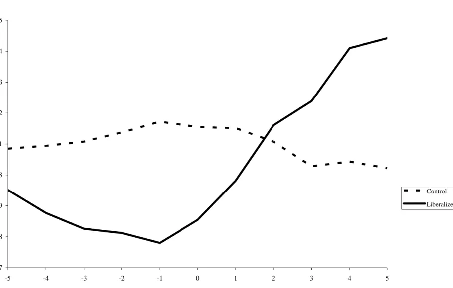
Figure 1 shows that in a sample of eighteen developing countries that opened their stock markets to inflows of foreign capital between 1986 and 1993, the average annual growth rate of the real wage in manufacturing jumped from 1.3 percent per year in non-liberalization periods to an average of 8.6 percent in the year liberalization occurred and each of the subsequent two years. The temporary 7.3 percentage-point increase in the growth rate of the real wage
permanently drives up the level of average annual compensation for each worker in the sample of liberalizing countries by about 752 US dollars—an increase equal to more than a quarter of their annual pre-liberalization salary.
One concern about Figure 1 is that an exogenous world-wide shock unrelated to opening
1
may drive up real wages in liberalizing and non-liberalizing countries alike. To distinguish the country-specific impact of liberalization policy from that of a common shock, our estimation procedure compares the difference in wage growth before and after liberalization to the same difference for a control group of countries not undergoing liberalization at the same time. In every specification, we find an economically and statistically significant increase in real wage growth for countries in the liberalization group but no effect for the control group.
Standard production theory provides the simplest explanation of the new facts that we document. Liberalization reduces the cost of capital, and firms respond by increasing their rate of investment. For a given growth rate of the labor force and total factor productivity, a higher rate of investment increases the ratio of capital per effective worker, driving up the marginal product of labor, and in turn, the market-clearing wage. Consistent with this interpretation, Figure 2 demonstrates that the growth rate of labor productivity also rises sharply in the aftermath of liberalizations. The average growth rate of labor productivity is 10.1 percentage points higher during the three-year liberalization window than in non-liberalization years. Again, the control group experiences no such increase.
While our difference-in-difference approach enables us to test for effects of liberalization on real wages and productivity that have previously gone unexamined, difference-in-difference estimation requires caution because the standard errors are susceptible to serial correlation. For instance, of the ninety-two difference-in-difference papers published in top economics journals between 1990 and 2000, only five explicitly address serial correlation (Bertrand, Duflo, and Mullainaithan, 2004). Peterson (2006) makes a similar point about panel data studies published in the top three finance journals between 2001 and 2004. The Bertrand et al. (2004) critique of difference-in-difference estimates applies with special force in the context of the liberalization
experiment examined in this paper.
Liberalizing the stock market increases investment, which in turn drives up productivity and wages. Because it takes time for wages to adjust, wage growth for a given country may remain elevated above its steady-state rate for a number of years in the post-liberalization period, thereby inducing serial correlation in the country’s wage-growth residuals over time. Similarly, liberalization often occurs at the same time across countries, thereby inducing correlation in the wage-growth residuals across countries at a given point in time. Our empirical analysis uses clustering techniques to adjust the standard errors for the occurrence of both forms of
dependence in the residuals (we also adjust for heteroscedasticity). No matter what specification we use, or how we compute the standard errors, the impact of liberalization on real wage growth remains economically and statistically significant for the treatment group and insignificant for the control group.
The potential endogeneity of the liberalization decision also raises some concerns. If profit-maximizing firms in a financially closed economy face the prospect of rapidly rising labor costs they will want to substitute capital for labor in the process of production. To the extent that liberalizing would reduce their cost of capital, these firms have an incentive to lobby the
government to do so. If rising wages cause governments to open up then our estimates will spuriously indicate a strong impact of liberalization on wages, when causation in fact runs the other way round. While theoretically plausible, the endogeneity argument has no empirical support. Figure 1 is not consistent with the view of liberalization as a response to rising labor costs. If anything, wage growth actually falls slightly in the run-up to liberalization (Section 5A shows that mean reversion à la Ashenfelter (1978) does not drive our results). The data are also not consistent with the explanation that governments liberalize in anticipation of higher future
labor costs. Although wages rise sharply in the aftermath of liberalization, labor productivity rises even faster, so that unit labor costs actually fall.
Finally, with only eighteen countries in the sample, one may worry that a few large outliers drive the central finding. This is not the case. In the aftermath of liberalizations, a temporary increase in real wage growth occurs consistently across countries. In all but three of eighteen countries, the median growth rate of real wages in the post-liberalization period exceeds the pre-liberalization median. Finally, the documented effects persist after controlling for
movements in the exchange rate and the impact of contemporaneous macroeconomic reforms such as inflation stabilization, trade liberalization, and privatization programs.
The rest of the paper proceeds as follows. Section 2 uses theory to generate testable predictions about liberalization and explains how we identify real-life liberalization episodes. Section 3 discusses the wage data and construction of the control group. Section 4 contains descriptive findings. Section 5 presents the main empirical results and evaluates the consistency of the estimates with standard production theory. Section 6 conducts robustness checks and considers alternative interpretations. Section 7 concludes.
2. Capital Account Liberalization in Developing Countries
This section generates empirically testable predictions about the impact of capital account liberalization in a developing country on the time-path of the real wage ( ). To maintain
congruency with previous work we employ the well-trodden framework of the neoclassical growth model, but apply it in a way that delivers previously untested theoretical predictions.
w
The central point about capital account liberalization is that it moves developing
of return to capital higher) than in the developed world, to a steady state in which capital-to-effective labor ratios and rates of return equal those in the developed world. Because capital and labor are complements in production, the marginal product of labor (and hence the real wage) rises as countries open up and the process of capital deepening sets in.
2A. Theory
Assume that the country produces output using capital, labor, and a constant-returns-to-scale production function with labor-augmenting technological progress:
(
,)
Y =F K AL (1)
Let
AL K
k = be the amount of capital per unit of effective labor and
AL Y
y= the amount of
output per unit of effective labor. Using this notation and the homogeneity of the production function we have:
( )
y= f k (2) Also assume that the country saves a constant fraction of national income each period and adds it to the capital stock, capital depreciates at the rateδ , the labor force grows at the rate n, and total factor productivity grows at the rate g.
When the economy is in steady state, is constant at the level k ks state. , and the marginal product of capital equals the interest rate (r) plus the depreciation rate:
. ( s state)
f k′ = +r δ (3) Because the impact of liberalization works through the cost of capital, equation (3) has important implications for the dynamics of and k w in the aftermath of opening up.
literature is that r* is less than r, because the rest of the world has more capital per unit of effective labor than the developing country. It is also standard to assume that the developing country is small, so that nothing it does affects r*. Under these assumptions, capital surges in to exploit the difference between r* and r when the developing country liberalizes.
The absence of any frictions in the model means that the country’s ratio of capital to effective labor jumps immediately from ks state. to its post-liberalization, steady-state level (ks state*. ). In the post-liberalization steady state, the marginal product of capital equals the world interest rate plus the rate of depreciation:
(
*)
*.
s state
f′ k = +r δ (4). Instantaneous convergence is an unattractive feature of the model, because it implies that the country installs capital at the speed of light. There are a variety of formal ways to slow down the speed of transition, none of which alters the fundamental predictions about wage growth in the aftermath of liberalization (Henry, 2007, Section 4.1).2 The vital point is that is greater than 0 during the country’s transition to its post-liberalization steady-state, and the temporary growth in k has implications for the growth rate of the real wage.
k
The growth rate of the real wage is the derivative of the natural log of with respect to
time, that is,
w
(ln ( ))
w d
w t
w= dt . Since workers are paid their marginal product of labor, . This means that the growth rate of the real wage is given by: [ ( ) '( )] w=A f k −kf k ( ) (ln( ( )) [ ( ) ( )] w d A kf k k w t w dt A f k kf k ′′ = = − ′ − .
We may write this expression as
2
1 ( ) ( ) w A f k k k w A σ f k k ′ = + i i (5) where ( )[ ( ) ( )] ( ) ( ) f k f k kf k f k f k k σ = − ′ − ′
′′ is the elasticity of substitution.
The right-hand-side of Equation (5) demonstrates that the growth rate of the real wage depends on the sum of two terms. The first term, the growth rate of total factor productivity
( A
A), is not affected by capital account policy in the canonical version of the neoclassical growth model (Gourinchas and Jeanne, 2006). In Section 5B we discuss the implications of recent work that adopts a more catholic view of the relationship between capital account liberalization and total factor productivity. For now, we proceed as though the impact of liberalization works strictly through the second term, which is the product of the inverse of the elasticity of
substitution (σ ), capital’s share in national income ( ( ) ( ) f k k
f k
′
), and the growth rate of the ratio of
capital per unit of effective labor (k k ).
Prior to liberalization, the ratio of capital to effective labor is constant at the level ks state. ,
so that k
k equals 0, and w simply grows at the same rate as total factor productivity. Since k k is greater than 0 during the transition to k*s state. , the growth rate of the real wage also increases temporarily. Figure 3 illustrates the hypothetical time paths of r and the natural log of k and w under the assumption that the interest rate converges immediately upon liberalization but the ratio of capital to effective labor does not.
The actual responses of the cost of capital, the quantity of capital and wages to liberalization resemble their hypothetical time paths. We know from previous work that
liberalization permanently reduces the cost of capital (Stulz, 2005) and temporarily drives up the growth rate of capital (Henry, 2003; Chari and Henry, 2008). Figure 1 shows that the growth rate of the real wage also increases temporarily. Later in the paper (Section 5B) we use Equation (5) to examine whether the magnitude of the estimated increase in the growth rate of the real wage is consistent with the magnitude of the previously documented increases in the growth rate of capital. The next subsection explains how we identify the real-life liberalization episodes used to construct Figure 1.
2B. Reality
Testing the prediction that real wage growth will rise following the removal of
restrictions on capital inflows requires information on capital account liberalization dates that is more precise than can generally be obtained. In theory, opening the capital account is as simple as pulling a lever. In reality, a country’s capital account has many components, so trying to determine exactly when it liberalizes the capital account (as in Section 2A) is perhaps the most difficult task in trying to assess the economic impact of changes in capital account policy.
In fact, the difficulty of determining precise liberalization dates causes most papers in the literature to ignore the problem (Eichengreen, 2001). Instead of asking whether opening the capital account has an impact on a country’s growth rate (as theory clearly dictates), most published studies examine whether openness and long-run growth are positively correlated across countries. A brief description of the data typically employed in such studies illustrates why tests of opening and openness are not equivalent.
To construct measures of openness, previously published work uses the broadest indicator of capital account policy available, the IMF’s Annual Report on Exchange
Arrangements and Exchange Restrictions (AREAER). The AREAER lists the rules and regulations governing resident and nonresident capital-account transactions in each country, a table summarizing the presence of restrictions, and a qualitative judgment on whether the country has an open or closed capital account. For the editions of AREAER published between 1967 and 1996, the summary table contains a single line (line E2) entitled, “Restrictions on payments for capital transactions.” The presence of a bullet point in line E2 indicates that the country has some form of restrictions on capital account transactions. In effect, line E2 delivers a binary judgment on whether the IMF considers a country’s capital account to be open or closed.
The typical study maps the qualitative information from Line E2 into a quantitative
measure of openness by tallying the number of years that each country was free from restrictions. Dividing that tally by the total number of years in the period produces a number called SHARE— the fraction of years over a given period that the IMF judged the country as open. For example, if a country was declared open for 15 of the 30 years from 1967 to 1996, then SHARE equals 0.5.
Papers that use the variable SHARE assess the economic impact of capital account policy by running cross-country regressions of GDP growth on SHARE. The problem with such regressions is that they implicitly test whether capital account policy has a permanent impact on growth while the theory predicts one that is temporary. The distinction between temporary and permanent has consequences. Cross-sectional regressions of growth on SHARE can generate spurious conclusions about the impact of liberalization on growth (Henry, 2007).
The cross-sectional approach to measuring the impact of capital account policy on growth is equally inappropriate for estimating the impact of liberalization on the growth rate of wages. Because theory predicts a short-lived impact of liberalization on wages, it is not enough to know
the fraction of years in which a country had an open capital account. We need to know the exact year in which the country opened up. In principle, one could look for the year in which the judgment in line E2 of the AREAER switches from “closed” to “open.” The problem is that when the AREAER changes an assessment from closed to open, it provides no information on the specific component of the capital account that was liberalized. Without such information the empirical implications of a change in openness are unclear.
For example, AREAER does not indicate whether the change in judgment about openness results from an easing of restrictions on capital inflows or outflows. The distinction matters. Theory predicts that when a capital-poor country liberalizes capital inflows it will experience a permanent fall in its cost of capital and a temporary increase in the growth rate of wages. In principle, if that same developing country were to liberalize capital outflows nothing would happen to its cost of capital, investment, or GDP.3
In contrast to the previous literature, this paper addresses the complexity of identifying liberalization dates by narrowing the scope of the problem. Instead of trying to determine the date on which the entire capital account switches from closed to open, it identifies the first point in time that a country liberalizes a specific component of the capital account. One example of liberalizing a specific component of the capital account is a decision by a country’s government to permit foreigners to purchase shares of companies listed on the domestic stock market. Liberalizing restrictions on the ownership of domestic shares enables foreign capital to flow into a part of the country’s economy from which it was previously prohibited.
Just such a policy change occurred repeatedly in the late 1980s and early 1990s, as a number of developing countries opened their stock markets to foreign investors for the first time.
3
For discussions of why this may not occur in practice, see Alfaro, Kalemli-Ozcan, and Volosovych (2008) and Shleifer and Wolfenzon (2002).
Removing restrictions on the ownership of domestic shares enables foreign capital to flow into a part of the country’s economy from which it was previously prohibited. Relative to the broadest conception of the capital account, the easing of restrictions on foreign investment in the stock market may seem like a parochial way to define capital account liberalization. But it is precisely the narrowness of stock market liberalizations that make them useful for testing the theory. As the previous paragraphs explain, changes in broad measures of capital account openness such as the AREAER provide a very noisy measure of liberalization policy. Since measurement error reduces the statistical power of any regression, it is important to focus on policy experiments where the true variation in the data is large relative to noise.
As the closest empirical analogue to the textbook example in Section 2A, stock market liberalizations provide just such experiments (Frankel, 1994). Accordingly, in this paper we use the year in which countries first opened their stock markets to foreign investors as the empirical counterpart to year “0” in the model of Section 2. According to Standard and Poor’s Emerging Markets Database, there are 53 developing countries with stock markets. Of these fifty three, eighteen have stock market liberalization dates that are: (a) consistently used elsewhere in the literature and (b) verifiable from primary sources. Column (1) of Table 1 lists these eighteen countries and the year in which they liberalized.4 Table 1 also presents summary statistics on the behavior of real wages in each of the eighteen liberalizing countries. The next section explains the source and construction of the wage data.
3. Data
The wage data come from the Industrial Statistics Database of the United Nations
4
For further details about the complexities of determining stock market liberalization dates see Section 5 of Henry (2007) and the other references therein.
Industrial Development Organization (UNIDO). UNIDO provides data on total wages and salaries, total employment and output for the manufacturing sector. For a given year, wages and salaries include all payments in cash or in kind paid to employees. Payments include: (a) direct wages and salaries; (b) remuneration for time not worked; (c) bonuses and gratuities; (d) housing allowances and family allowances paid directly by the employer; and (e) payments in kind. Excluded from wages and salaries are employers’ contributions on behalf of their employees to social security, pension and insurance schemes, as well as the benefits received by employees under these schemes and severance and termination pay.
Conceptually, total wages and salaries equal W*L*H, where W is the hourly wage rate, L is the stock of labor and H is total hours worked for the year. Since UNIDO provides no data on the number of hours worked or the hourly wage we divide total wages and salaries by total employment (L) to compute the average annual wage (W*H) in the manufacturing sector of each country. UNIDO reports the value of wages and salaries in US dollars, with the conversion from local currency made at the official nominal exchange rate. We deflate each country’s nominal annual wage in US dollars by the US consumer price index (CPI ) to create a dollar-denominated real wage.
In addition to information on wages, employment, and output, we would like to have data on the manufacturing capital stock. Unfortunately, UNIDO only provides data on investment. The standard approach to an absence of capital stock data converts investment flows to capital stocks with the perpetual inventory method by making assumptions about the initial level of capital in some year and using the investment flows to interpolate the subsequent time path of the capital stock.5
Interpolation is methodologically sound when the focus is on long-run relationships
5
where assumptions about the initial stock of capital make little difference. In contrast, this paper focuses on short-run dynamics and therefore requires a clear picture of the trajectory of the capital stock during the liberalization window. Simply put, it would be inappropriate for us to interpolate the growth rate of the capital stock during liberalization episodes when we are trying to measure the impact of liberalization on capital stock growth. Moreover, the UNIDO data set is missing more than 50 percent of the country-year observations for investment in the aggregate manufacturing sector, and many of these missing observations fall within the liberalization window. In the absence of reliable capital stock data, we will use (in Section 5B) estimates of capital stock growth from previously published work to check the consistency of our results with the theoretical channel from capital growth.
For each country in our sample, the annual wage data generally run from 1960 to 2003, with the exact dates differing by countries. After taking the difference of the natural log to compute growth rates, we have a total of 502 country-year observations with which to identify the impact of liberalization on real wage growth. Table 1 shows that the timing of liberalizations is correlated across countries, so these 502 observations are not entirely independent. For
instance, liberalizations may coincide with an exogenous global productivity shock that drives up wages in all countries, irrespective of whether or not they liberalize. To address whether this is the case we select a control group of countries in the manner described below.
3A. Construction of the Control Group
An ideal control group would consist of developing countries that are identical to the liberalizing countries in every respect except that the control countries did not open their stock markets to foreign investment. In practice, many of the developing countries that have stock
markets but never liberalized them are not appropriate for the task at hand. The purpose of the control group is to determine whether a global economic shock unrelated to opening up drives the temporary increase in real wage growth in the liberalizing countries. It is therefore critical that the control group not consist of countries in such an abject state of development that real wages would not respond to an external shock, no matter how favorable.
As it turns out, the list of forty-eight countries (see Appendix A) that have stock markets but never liberalized includes many countries at a low level of economic infrastructure such as Burkina Faso, Chad, Malawi, Sierra Leone, and Togo. Also, for those countries on the list of forty-eight that are at a similar stage of development as the liberalizers, their demarcation as non-liberalizers raises doubts about the reliability of the classification. For instance, Jamaica is classified as having never liberalized, but in 1987 one of the authors of this paper purchased stock there (as a naturalized US citizen).
In the absence of an ideal set of control countries, we use the liberalizing countries as their own control group in the following way. For a given liberalizing country, we define the control group as the subset of the eighteen countries in Table 1 that did not liberalize during the window of time that begins two years before and ends two years after the given country’s liberalization date. For example, Venezuela liberalized in 1990, so any country that did not liberalize between 1988 and 1992 appears in its control group. This subset consists of Chile, India, Jordan, Korea, Malaysia, Nigeria, the Philippines, Taiwan, Thailand, and Zimbabwe.6
Restricting the control group to countries that did not liberalize between years [-2, -1, 0, 1, 2] makes theoretical sense. The lion’s share of the impact of liberalization on wages occurs in years [0, +1, +2] (Henry (2007), Section 4.1). Therefore, the question is whether the real wage in liberalizing countries grows faster in years [0, +1, +2] than it does in countries that did not
6
liberalize during that time period. Countries that liberalized in years [-2, -1] are also excluded from the control group because the end of their liberalization period overlaps with the beginning of the given treatment country’s liberalization period.
To the extent that liberalization has a substantial impact on the real wage beyond year [+2], the methodology will bias our results against finding significant differences between the treatment and control group. To illustrate the potential bias, consider Venezuela and four members of its control group: Chile, Korea, Malaysia, and Thailand. Venezuela liberalized in 1990 while Chile, Korea, Malaysia, and Thailand all liberalized in 1987. This means that the third year after liberalization in those four countries is year [0] for Venezuela. If the impact of liberalization on wages in the four control countries persists into the third year after opening up, the difference between wage growth in Venezuela and the control group in year [0] will be artificially compressed.
Extending the control group restriction beyond two years would alleviate the problem of overlap, but for every given liberalizer, it would severely reduce the number of countries in the control group. In the end, we prefer to risk understating the significance of our results to using control groups that are not adequately large.
4. Descriptive Findings
Figure 1 dispels the concern that an exogenous global shock drives the liberalizing countries’ increase in real wages. The y-axis of Figure 1 measures the natural logarithm of the real wage. The x-axis measures years relative to liberalization. The solid line plots in
liberalization time the mean of the natural log of the real wage for all countries that liberalized. The dashed line plots the mean for the control group. Whereas the solid line exhibits a steep
positive inflection after year [0], indicating a sharp increase in the growth rate of the real wage, the dashed line remains flat as a pancake. While the flatness of the dashed line in Figure 1 suggests that a common global shock does not explain the inflection in the solid line, with only eighteen countries in the sample an important question is whether a few outliers drive the increase.7
Turning from means to medians, the data in Table 1 demonstrate that this is not the case. In the first year after liberalization (year [1]) five countries experience real wage growth that falls below the median growth rate of their real wage for the entire sample period. Under the null hypothesis that liberalization years are no different than non-liberalization years, the probability of finding no more than five countries below their median growth rate is 0.06. Similarly, in year [2], only five countries experience below-median annual real wage growth. Taking years [1] and [2] together, the probability of finding no more than ten episodes of below-median wage growth is 0.03.
Although the numbers in Table 1 suggest a consistent increase in real wage growth across countries, several other questions about the data remain.
First, the necessity of using annual instead of hourly wages raises a potential
measurement concern. If the average number of annual hours worked per employee increases following liberalizations, then total annual compensation may rise without any change in the implied hourly wage. In other words, the rise in annual labor income (W*H) documented in Figure 1 could be the result of an increase in hours worked rather than an increase in the hourly
7
We use the control groups to construct the dashed line in Figure 1 as follows. Fix a country and its corresponding liberalization date. For each element of the liberalizing country’s control group, calculate the natural logarithm of the real wage for the years in the interval [-2, -1, 0, 1, 2]. This yields a set of control-group-real-wage paths for the fixed liberalization-country. Next, for each year in [-2, -1, 0, 1, 2] calculate the mean over the entire set of all control-group-real-wage paths. Calculating these means creates a single path of the real-wage growth for the control group associated with the given liberalizing country. After repeating this procedure for each of the other seventeen liberalizing countries, we have eighteen control-group-real-wage-growth paths, one for each liberalizing country. The dashed line in Figure 1 is the average of all eighteen of these paths.
wage rate. To interpret the impact of liberalization on total annual compensation as an increase in labor’s compensation per unit of time, we need to know that the average number of hours worked does not rise significantly following liberalizations. Section 6 documents that we obtain similar results in a subsample of countries for which we have data (from a source other than UNIDO) on hourly wages.
Second, UNIDO reports salaries and wages in US dollar terms. In countries with high inflation, the rate of depreciation of the official nominal exchange rate may not keep pace with inflation. Under such a scenario, the real exchange rate appreciates and the dollar value of wages becomes artificially inflated. Similarly, liberalization itself may lead to a real appreciation, because opening the capital account generates a surge in capital inflows that strengthens the value of the local currency vis-à-vis the dollar. If liberalizations coincide with bouts of increased real appreciation, then the temporary rise in the growth rate of the real wage illustrated in Figure 1 may mechanically reflect changes in the bilateral real exchange rate rather than any
fundamental impact of capital account liberalization on the labor market. Figure 4 addresses the concern by replicating Figure 1 using wages measured in real local currency terms instead of real dollars. Since Figure 4 is virtually identical to Figure 1, indicating that the choice of currency makes little difference, the rest of the paper focuses on the real wage measured in dollars.
Third, liberalizations often coincide with major economic reforms that could have a significant impact on wages outside of any impact of liberalization. Stabilizing inflation, removing trade restrictions, and privatizing state-owned enterprises are all reforms that may affect real wages through their impact on the efficiency of domestic production. Indeed, Table 2 demonstrates that the timing of these reforms makes it plausible that they, not capital account liberalization, are responsible for the increase in real wages apparent in Figure 1. The next
section uses the information in Table 2 to control directly for the impact of other reforms and to address a host of lingering concerns and alternative explanations.
5. Empirical Methodology and Results
We evaluate the statistical significance of the temporary increase in wage growth by estimating the following panel regression:
0 1 2 3 4 5 ln * * * * * it i it it it it it it
w a COUNTRY a LIBERALIZE a CONTROL a TRADE
a STABILIZE a PRIVATIZE ε
Δ = + + + +
+ +
+
(6)
The left-hand-side variable, , is the natural log of the real dollar value of annual compensation for country i in year t minus the same variable in year t-1. Moving to the right-hand-side of equation (6), the constant measures average annual wage growth over the entire sample period after controlling for the country-fixed effects denoted by the variable .
lnwit Δ 0 a i COUNTRY The variable is a dummy variable that takes on a value of one in the year that country i liberalizes (year [0]) and each of the subsequent two years (years [1] and [2]). This means that the coefficient measures the average annual deviation of the growth rate of the real wage from its long-run mean over the three-year liberalization episode. is a
dummy variable that takes on the value one for all members of country i's control group during country i's liberalization episode. The coefficient measures the extent to which an exogenous shock having nothing to do with liberalization drives up wages in the liberalizing countries.
it LIBERALIZE 1 a it CONTROL 2 a
An alternative way of ensuring that the coefficient on the variable reflects the impact of country-specific liberalization policy and not that of a common shock would be to drop the control group variable and add year-fixed effects. We do this in Section 6, and the
it LIBERALIZE
results are virtually identical to the benchmark estimates from Equation (6).
Equation (6) constrains the coefficient on both the liberalization and control dummies to be the same across countries. A different approach would use a seemingly unrelated regression (SUR) to generate a unique set of coefficient estimates for each country. The problem with SUR is that it has low power. SUR also requires a balanced panel, and due to missing observations, creating a balanced panel would result in discarding a number of liberalization events. Given data limitations, the pooled cross-section time series framework is more appropriate.
The right-hand-side of equation (6) contains three additional dummy variables— STABILIZE, TRADE, and PRIVATIZE—that help to disentangle the impact of capital account liberalization from concurrent economic reforms. Wetreat reforms and liberalization
symmetrically, constructing dummy variables that take on the value one in the year a reform program begins and each of the two subsequent years.
Turning at last to the error term, εit, it is important to note that the standard distributional assumptions needed for valid statistical inference will not hold in the presence of: (a) correlation of the residuals across countries within a given time period, or (b) correlation of the residuals within a given country over time. Point (a) matters because liberalizations often occur at the same time for different countries, possibly inducing correlation in the wage-growth residuals across countries at a given point in time. Point (b) matters because it takes time for wages to adjust to their new trajectory; for a given country, wage growth may remain elevated above its steady-state rate for a number of years in the post-liberalization period, thereby inducing serial correlation in the country’s wage-growth residuals.
To compute standard errors that are correct, we construct clusters of residuals which allow for correlation within each cluster of observations. First, we cluster by year to produce
standard errors that account for the possibility that shocks to wage growth are correlated across countries within a given year. Second, we cluster by country to produce standard errors that account for the possibility that the shocks to wage growth are correlated over time within a given country. We also report estimates that correct for heteroscedasticity.
5A. Results
Table 3 (Panel A) shows that the impact of liberalization on real wage growth is economically large and statistically significant. The estimate of the coefficient on the
liberalization dummy ranges from 0.051 to 0.086. This means that during liberalization episodes the average annual growth rate of the typical country’s real wage exceeds its long-run mean by an average of 5.1 to 8.6 percentage points per year. Every estimate of the liberalization dummy in Panel A of Table 3 is statistically significant.
An exogenous shock to wages does not seem to drive the result. The estimate of the coefficient on CONTROL ranges from -0.011 to –0.02 and fails to attain statistical significance in every specification. An F-test confirms that the difference between the estimate of the
coefficient on LIBERALIZE and CONTROL is statistically significant at the one percent level in every specification in Table 3.
Controlling for the other economic reforms that tend to accompany liberalization also does not reduce the impact of capital account opening on the growth rate of the real wage. Column (5) in Panel A of Table 3 shows that after accounting for the effects of inflation stabilization, trade liberalization, and privatization, the coefficient on LIBERALIZE is 0.073. Because some of the economic reforms have a significant impact on the growth rate of the real wage, we are confident in the accuracy of the reform dates and the relevance of the
corresponding dummy variables as controls. For instance, the coefficient on STABILIZE is -0.088 and significant at the one percent level. The negative impact of stabilization programs on real wage growth is consistent with the literature on the real effects of inflation stabilization in developing countries.8
Finally, the significance of the estimates of the liberalization dummy presented in Panel A of Table 3 is also robust to the statistical concerns raised on page 19. Table 4 (Panel A) presents estimates that adjust the standard errors to account for heteroscedasticity. Table 5 (Panel A) presents estimates that adjust for heteroscedasticity and cross-country correlation. Table 6 (Panel A) presents estimates that correct for heteroscedasticity and serial correlation. None of these adjustments to the standard errors alter the results from Panel A of Table 3 in a material way. The liberalization dummy remains statistically significant in every specification of Panel A in Tables 4, 5 and 6. Because the statistical significance of the estimates of the
liberalization dummy are not sensitive to the method of computing standard errors, to economize on space, we turn our attention to the more central question of economic significance.
There are two ways to examine the economic significance of the results. First, consider the magnitude of the growth rate of the real wage during liberalization episodes relative to the growth rate of the real wage over the entire sample. To do this, use the estimate of the constant and the liberalization dummy from the regression that controls for other economic reforms (Column (5) of Panel A in Table 3). The estimate of the constant is 0.013, indicating that the real wage grows by an average of 1.3 percent per year over the entire sample. The estimate of the coefficient on the liberalization dummy is 0.073. Adding the constant and the coefficient on the liberalization dummy gives the average growth rate of the real wage during liberalization episodes—8.6 percent per year. This means that in the year the liberalization occurs and each of
8
the subsequent two, the average growth rate of the real wage in the typical country is almost seven times as large as in non-liberalization years.
Of course, the increase in the growth rate of the real wage is temporary, so a second way of assessing economic significance is to compute the impact of liberalization on the permanent level of the real wage. For the countries in the treatment group, the average level of annual compensation in the year before liberalization (year [-1]) is 2951 US dollars. During the three-year liberalization window the real wage grows at 8.6 percent per three-year, so that by the end of three-year [2] the level of the real wage is 2951 = 3820 US dollars. Now assume that that if the country had not liberalized the real wage would have grown by 1.3 percent per year. In that case, the end of year 2 the level of the real wage would be 2951 = 3068 US dollars. In other words, by the time the impact of liberalization has run its course, the average worker in the manufacturing sector has annual take home pay that is 752 dollars higher than it would have been in the absence of liberalization. This change in the level is greater than a quarter of the level of the average manufacturing worker’s pre-liberalization take home pay.
.086*3 e
.013*3 e
It is also important to note that the results do not simply reflect mean reversion following a temporary fall in earnings à la Ashenfelter (1978). While Figure 1 does show a gradual decline in the level of the real wage from years [-5 ] to [-1], a few hypothetical calculations demonstrate that the results in Tables 3 through 6 do not simply reflect a bounce-back effect. Five years prior to liberalization, the level of the real wage is 2,681 dollars. Now, suppose that instead of
declining for the next four years, real wages grew at their (continuously compounded) long-run rate (1.33 percent per year) for the next decade. Under that scenario, the real wage in year [+5] would be 3,063 dollars. The actual level of the real wage in year [+5] is 4,496 dollars, 38.4 percent higher than the level that would have prevailed had wages continued to grow at their
long-run rate. Simply put, the increase in the level of the real wage is too large to be an artifact of reversion to the mean.
5A.1 The Impact of Liberalization on Productivity
The response of wages to capital account liberalization is large. To scrutinize the
plausibility of our estimates we cross-checked the results against data on labor productivity. The model in Section 2 demonstrates that liberalization induces capital deepening, and through the increase in capital per worker, drives up productivity, the demand for labor, and the real wage. If this chain of reasoning has any empirical bite then during liberalization episodes labor
productivity should rise in concert with wages.
To formally test the relation between liberalization and the growth rate of labor productivity, we estimate the following regression:
0 1 2 3 4 5 ln( ) * * * * * it i it it it it it it Y
a COUNTRY a LIBERALIZE a CONTROL a TRADE
L a STABILIZE a PRIVATIZE ε Δ = + + + + + + + (7).
Equation (7) is identical to (6) except that instead of the change in the natural log of the annual wage, the left-hand-side variable is now the change in the natural log of value-added per worker.
Panel B of Table 3 shows that liberalization has a positive and significant impact on productivity growth. The estimates of the coefficient on the liberalization dummy range from 0.056 to 0.101. Every estimate of the coefficient on the liberalization dummy in Panel B of Table 3 is statistically significant. In contrast, the estimate of the coefficient on the control dummy is never significant. Taken together, these results suggest that liberalization, not an external shock or domestic economic reforms, is responsible for the increase in productivity growth.
In particular, Column (5) of Panel B in Table 3 demonstrates that after accounting for the potential impact of other economic reforms, the estimate of the coefficient on the liberalization dummy is 0.101. This means that the average growth rate of productivity is 10.1 percentage points higher during the three-year liberalization window than in non-liberalization years. The 10.1 percentage point increase in productivity growth associated with liberalization is larger than the 7.3 percentage point increase in wage growth. Because the increase in productivity outstrips the increase in wage growth, manufacturing-sector profitability actually rises during
liberalizations.9
5B. Discussion
While the size of the increase in productivity growth more than matches the size of the increase in real wage growth, the important unanswered question is whether the magnitude of either increase is consistent with the neoclassical model. To answer the question, begin with the standard assumption that liberalization has no impact on TFP growth and recall Equation (5):
1 ( ) ( ) w A f k k k w A σ f k k ′ = + i i .
With no change in the growth rate of TFP, the change in the growth rate of the real wage equals the product of three numbers: the reciprocal of the elasticity of substitution, capital’s share in national income, and the change in the growth rate of capital.
The capital share lies between 1/3 and 1/2. Obtaining an estimate of the change in capital growth requires a little more effort. We know from previous work that aggregate capital stock growth increases by 1.1 percentage points following liberalizations (Henry, 2003). We can use the aggregate number to calculate a rough upper bound for the change in manufacturing sector
9
capital growth. For the countries in our sample, the manufacturing sector accounts for 1/5 of GDP. Assuming zero net growth in capital for the agriculture and service sectors, the largest possible increase in the growth rate of capital in manufacturing is about 5.5 percentage points. This back-of-the-envelope calculation finds empirical support elsewhere in the literature. Using a subset of the countries in this paper, Chari and Henry (2008) calculate that the growth rate of capital in the manufacturing sector increases by 4.1 percentage points per year following
liberalizations. Increases in capital stock growth between 4.1 and 5.5 percentage points are also consistent with the size of the fall in the cost of capital that occurs following liberalizations.10
Suppose the capital share is 1/2 and the change in capital growth is 5.5 percentage points. Then for capital-deepening alone to explain the 7.3-percentage-point increase in wage growth you need an elasticity of substitution less than or equal to 3/8. If the capital share is 1/3 and the change in capital growth is 4.1 percentage points, then the elasticity of substitution must be less than or equal to 1/5. There is little consensus on the size of the elasticity of substitution. Early work estimated small elasticities that were statistically indistinguishable from zero.11 More recent studies cannot reject the hypothesis that the elasticity of substitution is 1 (Caballero, 1994). Most relevant to the countries in this paper, Coulibaly and Millar (2007) estimate an elasticity of substitution of about 0.8 for South Africa. With a standard error of 0.08, the Coulibaly and Millar estimate could imply an elasticity as small as 0.64. With a change in capital growth of 5.5 percentage points, a capital share of 1/2, and an elasticity of substitution of 0.64, Equation (5) predicts that liberalization would generate a 4.3 percentage-point increase in wage growth.
We do not mean to push any particular value for the capital share. And it is far from
10
See Henry (2007), pp. 897-900.
11
clear that we have a consensus estimate of the size of the elasticity of substitution in developed countries, let alone emerging economies. What is clear, however, is that if you want to maintain the orthodox assumption that liberalization has no impact on total factor productivity, then the observed increases in wage growth are consistent with the model only if you are willing to concede that the elasticity of substitution is less than 1 (i.e., the world is not Cobb-Douglas). But if the elasticity of substitution is significantly less than one, then it is hard to understand how profitability remains constant (or even increases slightly) following the liberalization-induced fall in the cost of capital.
On the other hand, if you maintain that the world is Cobb-Douglas, then our wage results necessarily imply that liberalization has a large impact on TFP growth. Indeed, if one is willing to step outside the confines of the Solow model there are plausible theoretical channels through which liberalization could raise total factor productivity. For instance, liberalization may enable firms to import more efficient machines (e.g., tractors instead of hoes) that effectively shift the country’s production technology closer to the world frontier. DeLong (2004) argues that after liberalizing the capital account “…developing countries…would enjoy the benefits from technology advances and from learning-by-doing using modern machinery.” In other words, to the extent that technological progress diffuses from developed to developing countries, the importation of new machinery provides an important conduit through which the diffusion may occur. Ninety-five percent of the world’s research and development (R&D) takes place in
industrial countries (Helpman, 2004, p. 64), and these same countries account for over 70 percent of the world’s machine exports in a given year (Alfaro and Hammel, 2007).
Evidence from the literature supports Delong’s conjecture that developing countries can import technological progress by liberalizing the capital account. In the immediate aftermath of
liberalizations, firms in the manufacturing sector of developing countries accumulate capital at a faster rate than they did before the liberalization (Chari and Henry, 2008). Furthermore, these countries raise their rate of capital accumulation by importing more capital goods. As a result of liberalization, the share of capital goods imports to total imports rises by 9 percent, and the share of total machine imports as a fraction of GDP rises by 13 percent (Alfaro and Hammel, 2007).
The observation that both imports of capital goods and total factor productivity rise in concert with liberalization lends credence to the notion that new capital goods embody
technological progress and that developing countries can raise their growth rates of total factor productivity by liberalizing the capital account.12 The observation is also consistent with work showing that: (a) the cross-country correlation between investment and growth stems primarily from investment in equipment and machinery (DeLong and Summers, 1991, 1993) and (b) cross-country variation in the composition of capital investment explains much of the cross-cross-country variation in total factor productivity (Caselli and Wilson, 2003).
Some argue that the simplest explanation of capital-account-liberalization-induced TFP growth lies with the economic reforms that accompany liberalization (Henry, 2003). Economic reforms improve resource allocation, essentially producing a one-time shift in the production function that temporarily raises the growth rate of TFP, without inducing technological process per se. Others posit that liberalization facilitates increased risk sharing, which might encourage investment in riskier, higher growth technologies (Levine, 1997; Levine and Zervos, 1998a). Yet another explanation is that capital account liberalization generates unspecified “collateral
benefits” that increase productivity (Kose, Prasad, Rogoff, and Wei, 2006).
Sorting through competing explanations for the increase in total factor productivity
12
Also, in the spirit of Rajan and Zingales (1998), liberalization may improve domestic firms’ access to external finance, which might in turn increase the rate at which firms import capital goods.
following liberalizations is an important research challenge that lies beyond the scope of this paper. The bottom line of this discussion is that the size of the increases in wage growth and productivity we report are consistent with the model that drives our estimation. Whether the primary source of those increases lies with capital deepening or increased total factor
productivity depends on reasonable differences in views about the elasticity of substitution that have yet to be resolved in the literature.
6. Robustness Checks/Alternative Explanations
To examine whether the significance of our results depends critically on our construction of the control group we adopt a different tack. We re-estimate the impact of liberalization by regressing wage growth on a constant, country-fixed effects, year-fixed effects, the liberalization dummy variable and dummy variables for the other reforms:
(8). 0 1 2 3 4 ln * * * * it i t it it it it it
w a COUNTRY YEAR a LIBERALIZE a TRADE
a STABILIZE a PRIVATIZE ε
Δ = + + + +
+ +
+
In Equation (8) the year-fixed effects now play the role that the control dummy variable played in Equation (6), preventing the impact of common global shocks to wage growth from inflating the coefficient on the liberalization dummy. We replicated all of the specifications in Tables 3 through 6 and obtained very similar results. The coefficient on LIBERALIZE is economically and statistically significant in every specification, and the point estimates range from 0.058 to 0.081. The same results hold when we estimate Equation (8) with labor productivity on the left-hand-side. The coefficient on the liberalization dummy is always significant and ranges from 0.057 to 0.102. To save on space we do not include tables with all of these additional estimates but they are available upon request.
6A. Alternative Explanations
One interpretation of the evidence says that wages rise following liberalizations because of an increase in labor demand stemming from a capital-deepening induced rise in productivity. Alternatively, the increase in wages may be due to a reduction in labor supply. The argument runs as follows. If workers perceive the impact of liberalization on wages to be permanent, then they effectively receive a positive shock to their permanent income and may reduce their labor supply accordingly.13 If this is the case then the observed increase in wage growth may stem from a decrease in labor supply as well as an increase in labor demand.
The employment data are not consistent with a decrease in labor supply. There is no discernible change in the growth rate of employment following liberalizations. We regressed the change in the natural log of employment on the same right-hand-side variables that appear in Equation (6), and the liberalization dummy was never significant.
We also looked at data on hours worked. If labor supply decreases then the number of hours worked should fall. In our attempt to see whether this is the case we had to rely on data for a smaller set of countries, because UNIDO does not provide data on hours worked. The
International Labor Organization (ILO) data was also not helpful, because the ILO’s definition of hours worked is inconsistent across countries and sometimes varies across sectors within a given country. In the end we obtained consistently constructed data on hours worked from the
Groningen Growth and Development Center (GGDC) for Argentina, Brazil, Chile, Colombia, Korea, Turkey, Taiwan, and Venezuela. We regressed the change in the natural log of hours worked on the same right-hand-side variables that appear in Equation (6). Again, the
liberalization dummy was never significant.
13
An alternative view is that labor supply is relatively inelastic (see Pencavel 1986 on this point). If this is the case, workers may not reduce the number of hours that they want to work in response to the increase in their expected future income.
The absence of a significant change in the number of hours worked also suggests that the increase in the growth rate of the annual real wage reported in Section 5A is not driven by a greater number of hours worked, but an increase in the rate of compensation per unit of time. As a final check we also used the GGDC data to construct a measure of hourly wages for the subset of countries mentioned above. Regressing the change in the natural log of the hourly wage on the same right-hand-side variables that appear in Equation (6), we find results that are
qualitatively identical to those reported in Panel A of Tables 3 through 6.
Overall, the evidence does not suggest that workers reduce their labor supply in response to liberalization. While we do not formally estimate the labor supply decision and cannot exclude the possibility that part of the wage increase results from a decrease in labor supply, if this alternative explanation is at work, its overall impact would appear to be second order.
7. Conclusion
Opening the stock market to foreign investment drives up real wages in the
manufacturing sector of developing countries without eroding profitability. Since workers gain, and owners of capital do not lose, the lingering question would seem to be: If liberalizing is such a good thing why do countries wait so long to do it? In trying to answer this question one has to be a little cautious.
The evidence in this paper applies only to manufacturing. In the absence of data on wages in agriculture or services, we cannot conclude that capital account liberalization improves aggregate welfare. Integration into the world economy during the 1980s and 1990s increased the ratio of skilled-to-unskilled wages in developing countries (Goldberg and Pavcnik, 2007). The possibility remains that easing restrictions on capital inflows contributed to the widening of the
gap. Therefore, while it may not cause distributive conflict within manufacturing, liberalization may create winners and losers across other sectors, with attendant political economy implications for the decision of whether and when to open up.14
Be that as it may, the evidence in this paper demonstrates that trade in capital has significant consequences for the real economy beyond its impact on prices and quantities of capital. All else equal, capital account liberalization raises the average standard of living for a significant fraction of the workforce in developing countries. As the quality and breadth of data on labor markets in developing countries continues to improve, future work may produce yet more definitive conclusions.
14
References
Alfaro, Laura and Eliza Hammel. 2007. “Capital Flows and Capital Goods,” Journal of International Economics, 72(1), 128-150.
Alfaro, Laura, Sebnem Kalemli-Ozcan, and Vadym Volosovych. 2008. “Why
Doesn’t Capital Flow from Rich to Poor Countries? An Empirical Investigation.” Review of Economics and Statistics, Forthcoming.
Ashenfelter, Orley. 1978. “Estimating the Effect of Training Programs on Earnings.” The Review of Economics and Statistics, 60 (1), 47-57.
Barro, Robert J. and Xavier Sala-I-Martin. 1995. Economic Growth, New York: McGraw Hill. Bertrand, Marianne, Esther Duflo, and Sendhil Mullainathan. 2004. “How Much Should We
Trust Difference in Difference Estimates?” Quarterly Journal of Economics 119(1), 249- 75.
Bhagwati, Jagdish. 1998. “The Capital Myth,” Foreign Affairs, 77, 7-12.
Caballero, Ricardo J. 1994. "Small Sample Bias and Adjustment Costs," Review of Economics and Statistics, 76, 52-58.
Caselli, Francesco and Daniel Wilson. 2003. “Importing Technology,” Journal of Monetary Economics 51 (1), 1-32.
Chari, Anusha, and Nandini Gupta. 2008. “Incumbents and Protectionism: The Political Economy of Foreign Entry Liberalization,” Journal of Financial Economics, Forthcoming.
Chari, Anusha and Peter Blair Henry. 2008. “Firm-Specific Information and the Efficiency of Investment” Journal of Financial Economics, Forthcoming.
Chirinko, Robert S. 1993. "Business Fixed Investment Spending: Modeling Strategies, Empirical Results, and Policy Implications," Journal of Economic Literature, 31, 1875-1911.
Cline, William R. 1995. International Debt Reexamined. Washington, D.C.: Institute for International Economics.
Coulibaly, Brahima and Jonathan Millar. 2007. “Estimating the Long-Run User Cost Elasticity for a Small Open Economy: Evidence Using Data from South Africa” Federal Reserve Board of Governors, Finance and Economics Discussion Series, 2007-25.
DeLong, J. Bradford. 2004. “Should We Still Support Untrammeled International Capital Mobility? Or Are Capital Controls Less Evil than We Once Believed?” The Economists’ Voice 1.
DeLong, J. Bradford and Lawrence Summers. 1991. “Equipment Investment and Economic Growth,” Quarterly Journal of Economics 106, 445-502.
DeLong, J. Bradford and Lawrence Summers. 1993. “How Strongly Do Developing Economies Benefit from Equipment Investment?” Journal of Monetary Economics 32, 395-415.
Eichengreen, Barry. 2001. “Capital Account Liberalization: What Do Cross-Country Studies Tell Us?” The World Bank Economic Review, 16(3), 341-365.
Fischer, Stanley. 2003. “Globalization and Its Challenges,” American Economic Review, 93(2), 1-30.
Fischer, Stanley, Ratna Sahay, and Carlos Végh. 2002. “Modern Hyper and High Inflations,” Journal of Economic Literature, 40(3), 937–980.
Frankel, Jeffrey A. 1994. “Introduction” in The Internationalization of Equity Markets, Jeffrey A. Frankel (ed), Chicago and London: University of Chicago Press, 1-20.
Goldberg, Pinelopi and Nina Pavcnik. 2007. Distributional Effects of Globalization in Developing Countries,” Journal of Economic Literature, 45(1), 39-82.
Gourinchas, Pierre Olivier and Olivier Jeanne. 2006. “The Elusive Gains from International Financial Integration,” Review of Economic Studies, 73(3), 715-741.
Helpman, Elhanan. 2004. The Mystery of Economic Growth. Harvard University Press, Cambridge, MA.
Henry, Peter Blair. 2000. “Stock Market Liberalization, Economic Reform, and Emerging Market Equity Prices,” Journal of Finance, 55(2), 529-564. Henry, Peter Blair. 2002. “Is Disinflation Good for the Stock Market?” Journal of
Finance, 57(4), 1617-1648.
Henry, Peter Blair. 2003. “Capital Account Liberalization, the Cost of Capital, and Economic Growth,” American Economic Review, 93(2), 91-96.
Henry, Peter Blair. 2007. “Capital Account Liberalization: Theory, Evidence, and Speculation,” Journal of Economic Literature, 45(4), 887-935.
Kose, Ayhan, Eswar Prasad, Kenneth Rogoff, and Shang-Jin Wei. 2006. “Financial Globalization: A Reappraisal,” NBER Working Paper No. 12484.
Levine, Ross. 1997. “Financial Development and Economic Growth: Views and Agenda.” Journal ofEconomic Literature, 35(2): 688–726.
Levine, Ross, and Sara Zervos. 1998a. “Stock Markets, Banks, and Economic Growth,” American EconomicReview, 88(3): 537–58.
Levine, Ross, and Sara Zervos. 1998b. “Capital Control Liberalization and Stock Market Development,”World Development, 26(7): 1169–83.
Obstfeld, Maurice. 1998. “The Global Capital Market: Benefactor or Menace?” Journal of Economic Perspectives, 12(4), 9-30.
Obstfeld, Maurice. 2007. “International Finance and Growth in Developing Countries: What Have we Learned?” Paper prepared for the Commission on Growth and Development. Pencavel, John. 1986. "Labor Supply of Men: A Survey", in Orley Ashenfelter and Richard
Layard, (eds), Handbook of Labor Economics, Volume I, North-Holland, 3-102. Peterson, Mitchell (2006). “Estimating Standard Errors in Finance Panel Data Sets:
ComparingApproaches.” Northwestern University Working Paper.
Rajan, Raghuram and Luigi Zingales. 1998. “Financial Development and Growth,” American Economic Review, 88(3), 559-586.
Rajan, Raghuram and Luigi Zingales. 2003. “The Great Reversals: The Politics of
Financial Development in the 20th Century,” Journal of Financial Economics, 59, 5-50. Rodrik, Dani. 1998. “Who Needs Capital Account Convertibility?” Princeton Essays in
International Finance, 207, 55-65.
Rogoff, Kenneth. 1999. “International Institutions for Reducing Global Financial Instability,” Journal of Economic Perspectives, 13(4), 21-42.
Sachs, Jeffrey and Andrew Warner. 1995. “Economic Reform and the Process of Global Integration,” Brookings Papers on Economic Activity, 1, 1-95.
Schoar, Antoinette. 2002. “The Effect of Diversification on Firm Productivity,” Journal of Finance, 62 (6), 2379-2403.
Shleifer, Andrei and Daniel Wolfenzon. 2002. “Investor Protection and Equity Markets,” Journal of Financial Economics, 66, 3-57.
Stiglitz, Joseph. 1999. “Reforming the Global Economic Architecture: Lessons From Recent Crises,” Journal of Finance, 54(4), 1508-1521.
Stulz, René M. 2005. “The Limits of Financial Globalization,” Journal of Finance, 60(4), 1595-1638.
Summers, Lawrence H. 2000. “International Financial Crises: Causes, Prevention, and Cures,” American Economic Review, 90(2), 1-16.
Figure 1. Real Wage Growth Rises in the Aftermath of Capital Account Liberalizations. 7.7 7.8 7.9 8 8.1 8.2 8.3 8.4 8.5 -5 -4 -3 -2 -1 0 1 2 3 4 5
Year Relative to Liberalization
ln ( R ea l Wag e in U S D o llars ) Control Liberalizer
Figure 2. The Growth Rate of Productivity Rises in the Aftermath of Capital Account Liberalizations. 10.3 10.4 10.5 10.6 10.7 10.8 10.9 11 -5 -4 -3 -2 -1 0 1 2 3 4 5
Year Relative to Liberalization
ln ( V al ue A d d ed p er W o rk er ) Control Liberalizers
Panel A: The Cost of Capital
Figure 3. Hypothetical Impact of Liberalization on the Cost of Capital, Investment and the Real Wage.
Interest Rate
r* r
t to
Panel B: Ratio of Capital to Effective Labor ln k( )
to t
ln(ks.state) ln(k*s.state)
ln(w)
Panel C: Real Wage
t to
Figure 4. Appreciation of the Real Exchange Rate Does Not Drive the Increase in Wage Growth. 7.7 7.8 7.9 8 8.1 8.2 8.3 8.4 8.5 8.6 -5 -4 -3 -2 -1 0 1 2 3 4 5
Year Relative to Liberalization
ln ( R ea l Wa g e in Lo ca l Curre n cy ) Control Liberalizers