Advertising, Pricing & Market Structure
in Competitive Matching Markets
Edner Bataille
yBenoît Julien
zFirst version: June 2003
This version: November 2005
Abstract
This paper develops a model of pricing and advertising in a matching environment with capacity constrained sellers. Sellers’ expenditure on directly informative adver-tising attracts consumers only probabilistically. Consumers who happen to observe advertisements randomize over the advertised sellers using symmetric mixed strate-gies. Equilibrium prices and pro…t maximizing advertising levels are derived and their properties analyzed, including the interplay of prices and advertising with the market structure. The model generates a unimodal (inverted U-shape) relationship between both, individual and industry advertising level, and market structure. The relationship results from a trade o¤ between a price e¤ect and a market structure-matching e¤ect. We …nd that the decentralized market has underprovision of advertising, both for in-dividual sellers and industry wide, and that entry is excessive relative to the e¢ cient level. We present a quantitative analysis to highlight properties of the models and to demonstrate the extent of ine¢ ciency.
JEL codes: B21, C72, C78, D40, D43, D61, D83, J41, L11, M37.
Keywords: Advertising, pricing, market structure, endogenous matching, asym-metric information, e¢ ciency.
We would like to thank Pedro Gomis-Porqueras, John Kennes, Kei Hirano and Luis Locay for useful comments. The usual disclaimer applies.
yCalifornia State University-Bakers…eld, Department of Economics, ebbataille@yahoo.fr
zAustralian Graduate School of Management, and CAER, University of New South Wales and University of Sydney, Australia, e-mail: benoitj@agsm.edu.au
1
Introduction
We analyze the equilibrium relationships between advertising, pricing and market concen-tration in a market in which there are frictions. The market has N identical consumers and
M identical sellers. Each consumer wants to buy one unit and each seller wants to sell one unit of an indivisible good. Each seller must advertise in order to be known to consumers. Each advertisement contains location, capacity and price information.1 Based on the ads observed, consumers select one and only one seller with whom they want to trade. Then all trades occur at the advertised prices. Frictions arise in this kind of market from the fact that sellers have a capacity constraint, and consumers are uncoordinated in decisions to select a particular seller. The implication is that a particular seller might be selected by more then one consumer, in which case all but one consumer faces rationing. Models of this sort, but without explicit costly advertising have become known as markets in which sellers choose their price and probability of service. Examples of such models include Peters (1991), Deneckere and Peck (1995), and more recently Burdett, Shi and Wright (2001)2.
This paper uses the framework of Burdett, Shi and Wright (2001), but modi…ed to include the more realistic feature of explicit advertising choices by sellers. It is assumed that adverting is costly and that ads sent by sellers are observed by each consumer probabilistically as in Butters (1977). Without advertising (and consumer search), sellers would not be able to sell, and the market would not exist. The general idea conveyed by Butters (1977) advertising technology is one of "hit and miss" feature of advertising. The interpretation is that each consumer may not truly pay attention to the advertisement. Common examples are consumers who trash mailbox ‡iers before reading them, or uses television advertising time during a program to do something else. Therefore, when sellers send advertisements, only a fraction of consumers will get to observe at least one of the ads, and hence the returns on advertising expenditure is probabilistic.
We investigate how this type of advertising is in‡uenced by equilibrium prices and by the consumers to sellers’ratio, which we refer to as market concentration.3 In models of price and probability of service, the extent of frictions is in‡uenced by the consumers to sellers’ ratio. We are interested in how advertising and pricing are in‡uenced by the presence of frictions, as well as how advertising in this environment a¤ects the matching rate.
The model is simple enough to allow for the derivation of the closed form for the equi-librium advertising level, prices and matching rate, as a function of market concentration. Since we assume homogeneity on both sides of the market, all sellers choose the same level of advertising and pricing, and all consumers use the same mixed strategy over sellers from whom they have observed at least one ad.
1This is a model of directly informative advertising. For a recent survey on di¤erent forms of advertising
see Bagwell (2001).
2Some models exist assuming competition in auctions using reserve prices such as McAfee (1993) and
Peters and Severinov (1997). There are also models applied to the labor market such as Ciao and Shi (2000) and Julien, Kennes and King (2000).
3Competitive intensity is measured by the number of sellers relative to the number of consumers. Since
We …nd that equilibrium advertising is in‡uenced by equilibrium market price positively as intuition dictates. Higher price makes costly advertising more worthwhile. But the mag-nitude of the impact depends on the market concentration. Markets with substantially less sellers then consumers (concentrated), yields a larger impact of price on advertising level then markets with substantially more sellers then consumers (competitive). This occurs because the equilibrium price is concave in market concentration (convex in the number of sellers). We also …nd equilibrium advertising to have a unimodal relationship with market concentra-tion. Advertising per seller, and at the industry level reaches its peak for intermediate values of the ratio of consumers to sellers. For extreme values of the ratio, advertising converges to zero. Therefore for very slack or tight markets, advertising is found to be minimal. In other words, it suggests that peak advertising would be observed in oligopolistic markets. This result is driven by the nature of the matching environment. The derived matching function implies that for a given number of consumers, the probability with which a seller is visited by one consumer is lower when either there are numerous or a small number of sellers. The former is obvious since numerous sellers implies a very low probability a consumer will select a particular seller. Hence, it makes advertising less worthwhile. In the latter case, when there are too few sellers, the probability with which a consumer will select a particular seller is high, meaning that each seller is more likely to be visited by several consumers. Hence, no need to advertise much. There exist a good body of empirical literature empha-sizing the causality that concentration in‡uences advertising showing signi…cant non-linear relationships, inverted U-shape, between concentration and advertising, as reported in the extensive survey from Bagwell (2003). Buxton, Davies and Lyons (1984) and Uri (1987) also provide empirical support for an inverted U-shape relationship especially for industries where a greater proportion of sales go to …nal consumers. In our model, all sales go to …nal consumers.
This paper is closely related to Butters (1977). We use his advertising technology and also assume a unit demand for each consumer. However, Butters (1977) does not have capac-ity constraint and our consumers are strategic, using mixed strategies in selecting sellers. In fact, introducing limited capacity along with an endogenous matching technology to analyze equilibrium advertising intensity is what di¤erentiates this paper from all the literature.4. Stegemen (1991) essentially extends Butters’s (1977) model to the case of consumers het-erogeneous reservation values and assume large number of buyers and sellers. Stahl (1994) considers …nite number of buyers and sellers and allows for downward sloping individual demand curve and a general advertising technology. He considers the in‡uence of consumers to sellers’ratio on the price and advertising distributions. He …nds, as in this paper, that more sellers imply lower prices, but less advertising per seller, as opposed to a unimodal relationship. The models of Stegemen and Stahl do not have capacity constraint also. These three models su¤er from the standard non-existence in pure strategy equilibrium in prices for sellers due to the fact that sellers’s payo¤s are discontinuous when prices are equal.
4Our model is also suitable for analyzing competition in sales (advertised price discounts) with limited
Hence, they resort to mixed strategy equilibrium in prices, generating price dispersion as a consequence. The matching environment assumed in this paper alleviated this discontinuity problem and allows for unique symmetric equilibrium price to be derived. Finally, none of these papers show an unimodal in‡uence of concentration on advertising, which is a main contribution of this paper.
Remarkably Butters (1977) has shown advertising to be e¢ cient in his model. Stahl (1994) also …nds advertising to be e¢ cient when considering a unit demand as in our model. Here, as in Stegemen (1991), we …nd underadvertising relative to the e¢ cient level. Moreover, we show how this result extends to the industry level of advertising. The main reason for ine¢ cient advertising is well known in search models. On one hand the search cost (advertising cost) is born entirely by sellers while the bene…ts are shared by both consumers and sellers upon a match. This induce less than socially optimal advertising. On the other hand, there is a business stealing e¤ect when a seller sets a lower price then others, and this externality generally tend to cause excessive advertising. Butters (1977) …nds that these two e¤ects cancel, while the search cost dominates in Stegemen (1991) and Stahl (1994). We …nd in this paper, with limited capacity and endogenous matching, that search cost also dominate to create underadvertising relative to the e¢ cient level for any market concentration levels. Furthermore, we show that there is excessive entry relative to the e¢ cient level. Finally, we show how an entry tax and an advertising rate subsidy can induce e¢ ciency of advertising and entry within a balanced budget.
The following sections are organized as follows: Section two presents the basic model with consumers and sellers’choices. Section three assesses the e¢ ciency of advertising and entry. Section four considers a numerical simulation of the model. A discussion and conclusion follows.
2
The Model
The model consists of a large numberM of identical sellers each carrying only one unit to sell, and a large numberN of identical potential consumers each with a unitary demand. We refer to the ratio of consumers to sellers =N=M as the market tightness or size-concentration5. The number of sellers M and consumers N is assumed common knowledge to all sellers and consumers. However, we assume that sellers know also each others’s identity, but consumers do not know sellers’identities. Each seller must advertise in order to be known to consumers. They do so by sending a number of ads or messages,s, and each consumers observe the ads only probabilistically. Each consumer has interest in purchasing from a particular seller if and only if he has observed at least one ad from that seller. Consequently, the advertising
5Reference to as market tightness is more commonly used in search models of the labor market using a
matching function. In this paper we refer to it as size-concentration. The reason is as follows. Let ibe each
seller’s market share. The Her…ndahl-Hirschman Index of market concentration is HHI =PMi=1 2i. This index has the property that if the …rms are identical, in this model i= 1=M for alli, then theHHI= 1=M.
Then we refer to = (HHI)N as a measure of market concentration. One can also use the C1 = 1=M concentration ratio to form =C1N.
rate is de…ned as a =s=N. Each ad only contains information about location/identity and price for the seller. We assume that the product features are common knowledge and focus on search goods and directly informative advertising, abstracting from issues of advertising as a signal of quality, product related informational asymmetries and persuasive advertising.
The structure of the model is described by the following sequence of events:
1. Each seller i chooses jointly an advertsing rate ai =si=N and a price pi to maximize
expected pro…ts, taking as given other sellers’s choices.
2. Each sellerisends a number of adssi in order to reach and attractN consumers. Each
ad contains the seller’s identity, location and price informationpi.
3. Each consumer observes at least one of the ads from each particular seller with proba-bility h=h(ai) given the advertising rate ai chosen from that seller based on a given
number of consumersN. This probability is common knowledge and will be explicitly derived in the next section.
4. Upon observing locations and prices from a set of sellers’ads, each consumer selects one and only one particular seller i from which to purchase with probability i(p),
where (p)is the observed price vector from a set of sellers.
5. Whenever matches are formed, transactions are performed at the advertised prices. In order to solve the model, we focus on symmetric equilibria in which all sellers choose the same price and advertising rate, and consumers select over sellers using mixed strategies. This particular structure implies a tradeo¤: consumers try to minimize competition at a seller, but sellers try to maximize it. In other words, consumers select over sellers trading o¤ a price and a probability of trade.
2.1
Advertising Technology and Consumer Choice
In this section we derive a typical consumer’s choice. We assume that consumers know the total population of sellers, M, but do not know the identity or location of any particular sellers, and hence, the availability of a product and price, until they have seen ads from them. A consumer’s choice is then a selection of a particular seller from which to purchase an item once it has observed at least one ad. However, we assume that not all sellers’s ads are observed by consumers. In order to capture this feature we adopt a speci…cation of an advertising technology based on the model of Butters (1977). Assuming that each consumer observes an ad or a signal with probability1=N, then(1 1=N)is the probability to observe no ads. If a seller send a number of adss, then(1 1=N)s is the probability to observe none of thesads sent by a seller. Since we focus on large markets, taking the limit of(1 1=N)sas N andsgo to in…nity but keeping the ratios=N …xed, the probability with which a consumer does not observe any of thesads ise s=N. Therefore, the probability to observe at least one of
thesads from a particular seller is(1 e s=N). Using the advertising ratea =s=N, we write h(a) = (1 e a)and note that this probability is independent of advertising rates performed
by other sellers. This seems natural in the context of directly informative advertising where it only conveys information about a particular seller’s identity, location, price and possibly other informative features. This advertising technology is only one way to represent how sellers search for consumers. It also considers consumers as passive in the sense that they do not take any actions to increase the probability to observe a seller’s advertisement. Although we could introduce costly consumers search, for example by allowing them to sample more communication media, or simply searching for prices as in Robert and Stahl (1993), we focus on search intensity on the sellers’side. This is equivalent to assuming that the net bene…ts of searching for sellers is negative for consumers. This may be explained by high opportunity cost of search such as work hours and/or home production.
The immediate implication of introducing an advertising technology is that each consumer
j gets to observe at least one ad, and hence, prices from a set of sellersmj
f0;1; :::; Mg. Let#mj be the cardinality of the setmj. If#mj = 0 consumerj recieved no ads at all and
isUninformed. If#mj = 1, consumerjhas observed ads from only one seller so he iscaptive,
implying j(p(mj)) = 1. When consumer j observes ads from several sellers, #mj >1, he
is selective and uses a mixed strategy. Since mj is private information to consumer j, for
any vector of advertising rates a, using the probabilities h(ai) for each seller i, one obtains
the probability with which consumerj observes mj as !(mj;a) = M mj mj Y =1 h(a ) M Y `=mj+1 (1 h(a`)): (1)
Consumer j’s strategy consists of selecting one and only one seller with probability
j(p(mj)) where p(mj) = (p
1; :::; pmj) is the observed price vector from the mj sellers,
and Pmi=1j ji(p(mj)) = 1. That is consumers use mixed strategies over their set of known
prices. The probabilities !(mj;a) can be used to form a discrete probabiltity distribution
over the possible mixed strategies ji(p(mj)) 8mj f0;1; :::; Mg. From this distribution one can obtain the probability that any one of the M sellers be observed and selected by consumer j as j (p;a) = M X mj=1 !j(mj;a) j(p(mj)) (2) where (p;a) = (p1; :::; pM; a1; :::; aM). This probability simply represents the fact that j(p(mj))used by each consumerjis private information, and hence, j(p;a)is the expected
mixed strategy of consumer j. Symmetry on the consumers’side implies j(p;a) = (p;a)
for all j and any vectors p and a.
When selecting a particular selleri2mj, a consumer needs to assess the probability with which other consumers select seller i. This probability depends on how many other sellers
these consumers have observed as captured by the probabiltiy (p;a). This probability also depends on the vectors of advertising and prices. However, consumers do not observe the vector of advertising rates a and may not get to observe the overall price vector p. Letting p(M) = (p1; :::; pM) be the overall price vector, then p(Mnmj) is the set of prices
not observed by consumerj. Therefore, any other consumer who has observed a pricepk 2
p(Mnmj) will select seller k with positive probability and the actual price set by seller
k will in‡ence the mixed strategy they use. Consumer j must form expectations about advertising rates, but also about unobserved prices based on his set of observed prices. That is, a consumer forms the following expectations E(p(Mnmj)) = p~(Mnmj) and E(a) = ~a
which he uses to evaluate the probability with which other consumers observe and select a particular seller i. For example, a consumer who has observed seller i 2 mj and selects
this seller with probability ji will make the following calculations about other consumer `’s probability to observe and select seller i:
~` i(p(m j);~p(M nmj);~a) = M X m`=1 !`i(m`;~a) `i(p(mj \m`);~p(m`nmj)): where !i(m`;~a) = mM` m` Y =1 h(~a ) M Y `=m`+1
(1 h(~a`)) and p(mj \m`) is the price vector
com-monly observed by any two consumersj and`, and~p(m`
nmj)is the vector of prices observed
by consumer ` and not by consumer j, but has formed expectations over it. Under symmetry and assuming rational expectations~`i(p(mj);p~(M
nmj);~a) = `
i(p;a) =
(p;a) for all ` and for all i.
Assuming that each consumer extracts a utility value normalized to 1 from consuming the good, the consumer surplus from selecting seller i is (1 pi). Since each seller carries
only one unit of the good to be sold, the rationing rule is such that when several consumers select the same seller, each one get the good with equiprobability. Consumers’selections and the rationing rule translate into a probability ji to get served which depends on the number of other consumers also selecting selleri.
A consumer j’s expected utility from selecting selleri is
Uij(p;a) = (1 pi) ji(p;a): (3) We focus on mixed-strategy equilibrium selection for consumers. (See Burdett, et al. (2001).) The mixed-strategy equilibrium selection is such that a consumer is indi¤erent between selecting any two observed sellers. For any given vectors of prices and advertising rates(p;a)set by sellers, a mixed-strategy equilibrium selection for any consumerj = 1; :::N
is a vector of probabilities j(p) = ( j
1(p); :::;
j
mj(p))solving
Uij(p;a) = Ukj(p;a) (4) for all i; k 2 mj, such that Pim=1j ji(p) = 1. Unlike the model of Burdett et al. (2001), advertising generates a distribution of these equilibrium mixed strategies.
The probability with which consumer j gets served when selecting seller iis j i(p;a) = N X ni=1 1 ni+ 1 N 1 ni i(p;a)ni(1 i(p;a))N 1 ni: (5)
whereni is the number of consumers (excluding consumerj) who have selected selleri, and
1
ni+1 is the rationing rule.
To simplify this probability, consider the probability that a consumer is alone selecting seller i, which occurs when ni = 0,
Prfni = 0g= (1 i(p;a))N
and the probability of not being alone selecting seller i is
Prfni >0g= 1 (1 i(p;a))N
Using this simpli…cation,6
i(p; a) = h 1 (1 i(p;a)) Ni N i(p;a) :
The probability to get served at selleriis the probability that at least someone has seen the ad and selects selleri, (1 (1 i(p;a))N, times the probability to "win" the item N 1
i(p;a),
6Since probabilities sum to one
Prfn >0g= NX1 n=1 N 1 n n (1 )N 1 n= 1 (1 )N 1
is the probability that at least one other consumer observes the ad of a seller and selects that particular seller. Using this simpli…cation along with the rationing rule, the probability to get served is transformed as follows: (p; a) = "N 1 X n=1 1 n+ 1 N 1 n n(1 )N 1 n # = 1 N NX1 n=0 N n+ 1 n (1 )N 1 n = 1 N N X n=1 N n n (1 )N n = (1 (1 ) N ) N :
where N i(p;a) is the expected number of consumers who have observed and selected that
seller.
Since there are M sellers in the market from which advertisements can potentially be observed, we have M X i=1 i(p;a) = 1 M Y i=1 (1 h(ai)) (6)
where the term
M
Y
i=1
(1 h(ai))simply re‡ects the possibility that a consumer observed no ads
at all. If all sellers set the same advertising rate a then
M
Y
i=1
(1 h(ai)) = (1 h(a))M.
Suppose now that a deviant seller sets price p^while all other sellers set price p, but all sellers set the same advertising rate. This yields ^ + (M 1) = 1 (1 h(a))M and the
probability with which a consumer oberves and is expected to select any of the non-deviant sellers is = 1 ^ (1(M h1)(a))M.
The expected utility from observing and selecting the deviant seller is
^
U(^p;p 1;a) = (1 p^)
1 1 ^
N
N^ : (7)
Similarly, the expected utility from selecting a non deviant seller is
U(^p;p 1;a) = (1 p)
1 1 1 ^ (1M h1(a))M
N
N 1 ^ (1M h1(a))M
: (8)
A symmetric, mixed-strategy, equilibrium selection ^(^p;p 1;a)solves:
U(^p;p 1;a) = ^U(^p;p 1;a) (9)
However, explicit solutions for (p;a) is characterized by a polynomials of high degree and cumbersome to handle.7 Fortunately, the explicit solutions are not needed for the equilibrium derivations. All we need is the conditions under which a mixed strategy equilibrium selection exist. It can be shown that as long as the price deviation is not too small or not too big, there is a unique ^2(0;1)that makes consumers indi¤erent between the deviant seller and the non-deviant seller.8
7This property of (p; a) is particular to the use of a posted price mechanism. When using auctions or
ex post bidding, these probabilities have explicit solutions (see Julien, Kennes, and King (2000, 2005).
Lemma 1 The unique symmetric mixed-strategy equilibrium when pi =p and ai =a for
all i is ji = 1=mj for all j and for all mj
2 f1; :::; Mg.9
In a symmetric mixed-strategy equilibrium in which all sellers choose the same advertising rate a and price p , the unique expected selection strategy is = ^ = = 1 (1 Mh(a ))M.
In this model, we focus on mixed strategy equilibrium in order to capture the feature that consumers’decisions are uncoordinated. While coordination is a more probable behavior in small markets, in large markets this is unlikely and harder to implement. This is equivalent to assuming a communication technology constraint preventing consumers from coordinating on their selection strategies. In this model there are pure selection strategy equilibria. But the implementation of these equilibria would require a coordination technology that we assume away here.
2.2
Equilibrium Prices and Advertising Rates
Equilibrium market price
Each seller jointly chooses its price and advertising rate simultaneously to maximize expected pro…ts, taking as given other sellers’s choices, andexpected consumers’behavior.10 In order to be active on the market, each seller must incur a …xed costF 2[0;1], which may or may not be associated with advertising as in the cost of setting up a selling location.11 Each seller faces a variable cost c(a) for an advertising rate of a, with constant marginal cost, that is c0 >0 and c00 = 0. The expected pro…t for a seller is
(p;a) =pq(p;a) c(a) F (10) where q(p;a) = 1 (1 (p;a))N is the probability of sale. Sellers use the probability
(p;a) to derive the probability of sale since they do not know consumers’ exact mixed strategies. Finding the symmetric equilibrium market price involves solving a set of M
reaction functions. Instead we use the technique in Burdett, Shi and Wright (2001) which
9
For a proof of this Lemma see Burdett etal. (2001).
10McAfee (1994) considers a two–stage game theoretic model where …rms choose advertising …rst and
prices in the second stage. However, for a model considering simultaneous choices see Robert and Stahl (1993).
11Fixed costs associated with advertising are sunk costs. Advertisements are costly to set up, or more
generally a marketing campaign needs preparation. However, even for industries where …xed costs associated with advertising may not be present or even minimal, the …xed cost we introduce can be taken as …xed cost for a seller to be on the market, such as cost of setting up the shop/location. Given the constant marginal cost assumption, there are economies of scale in advertising. This is consistent with existing communication technologies.
is to assume as above that all sellers but one set a price p and advertising rate a, while a deviant seller sets price p^. The objective of a deviant seller is
max
<p>^ ^ (^p;p 1;a) = max<p;a>^ fpq^ (^p;p 1;a) c(a) Fg, (11)
where now q(^p;p 1;a) = (1 (1 (^p;p 1;a))N). Consider …rst the pricing decision,
taking the price pand advertising ratea of all other sellers as given. The pro…t maximizing deviation satis…es @^ @p^ =q(^p;p 1;a) + ^p @q(^p;p 1;a) @p^ = 0: (12) or 1 1 ^ N + ^pN 1 ^ N 1 @^ @p^= 0 where @^ @p^ = PM m=1!(m;a) @ (^p;p 1(m 1)
@p^ . The second-order condition is satis…ed sinceq(^p;p 1;a)
is concave in p^. Assuming ^2 (0;1), di¤erentiating (9) with respect to p^and inserting the symmetric equilibrium conditions p^=p, and a for all sellers, and ^ = = 1 (1Mh(a))M yields
@^ @p^= (M 1) (1 (1 h(a))M)(M (1 (1 h(a))M)) 1 M (1 (1 h(a))M) M N M2(1 p) M 1 M (1 (1 h(a))M) M N (M + (N 1) (1 (1 h(a))M)) <0: (13) Inserting this into (12), yields
p (M; N;a) = M M M+(MN(1 (11)(1 (1h(ah))(Ma)))M) M (1 (1 h(a))M) M N M M2 M(M(1 (1N)(1 (1h(a))hM(a)))M) M (1 (1 h(a))M) M N : (14)
The equilibrium price in …nite markets depends on the advertising rates. It is easily shown that p (M; N;a) is strictly increasing in a, meaning that higher advertising rates by all sellers translates into a higher equilibrium market price. This simply means that if all sellers choose more advertising, they choose a higher price in equilibrium to generate the expected revenue to compensate for the extra advertising expenditure. In large markets the equilibrium price p (M; N) converges very quickly to
p ( ) = lim
M;N!1p (M; N) = 1 e 1: (15)
which is the same limit price found by Burdett, Shi and Wright (2001). Therefore, in large markets, the in‡uence of advertising on equilibrium prices becomes insigni…cant as one would expect.
Properties of the equilibrium market price
The equilibrium market price p ( ) is strictly increasing and strictly concave in with limits
lim
!0p ( ) = 0 and lim!1p ( ) = 1: (16)
Furthermore, p ( ) converges quickly to its limit value of1. For instance a value = 10is enough to havep ( )very close to1. Since we have an equilibrium market price determined by concentration, we can de…ne the elasticity of market price with respect to concentration as ( ) = @p@( )p ( ), which is always positive, along with properties that ( ) is strictly decreasing in , with lim
!0 ( ) = 1 and lim!1 ( ) = 0. These properties indicate that as
the market becomes less competitive, higher , the equilibrium market price increases and this price becomes less sensitive to a further decline in competition. In other words, with a large consumer to seller ratio, an exit by one seller will not have much of an impact on the equilibrium price. However, when such a ratio is small, an exit by one seller creates a bigger impact on the equilibrium price.
Equilibrium advertising rates
Each seller now chooses an advertising rate ^a, given their choices of price p, and taking as given all other sellers choices of advertising ratesa 1 and prices p, to solve:
max ^ a (p;^a;a 1) = maxa^ fp( ;a)q(p;^a;a 1) c(^a) Fg where q(p;^a;a 1) = h 1 (1 (p;^a;a 1))N i
. The …rst-order condition is
@^ @^a = @p(M; N;a) @^a q(p;^a;a 1) +p @q(p;^a;a 1) @^a @c(^a) @^a = 0; (17)
which is the standard marginal revenue equals marginal cost of advertising rate. Note that
@q(p;^a;a 1) @^a = N(1 (p;^a;a 1)) N 1 @ (p;^a;a 1) @^a , and @ (p;a;a^ 1) @^a = PM m=1 @!(m;^a;a 1) @^a (p(m)) = (p;a)h0(^a)
h(a) > 0, meaning that a higher advertising rate by a seller increases the probability
to be observed and selected, but not the conditional probability to be selected once the consumer has observed at least one ad, that is (p). This is the nature of informative advertising. Here, once a consumer has observed at least one ad from a seller, a higher advertising rate cannot induced consumers to change their mixed strategy (p)in his favor. If we were to allow for this e¤ect, advertising would need to have a persuasive element.
The …rst-order condition yields the reaction function
@p(M; N;a)
@a^ q(p;^a;a 1) +p(M; N; a)N(1 (p;^a;a 1))
N 1 @ (p;^a;a 1)
@^a =c
The second-order condition is satis…ed since h(a), and hence q(p;a), are concave in a. Under symmetric equilibrium p = p and ^a = a for all M with (p ;a ) = 1 (1Mh(a )), where p is de…ned in (15). Assuming a total cost of advertising of c(a) = a, and using
h0(a) = e a, the …rst-order condition becomes
@p(M; N;a)
@^a q(p;^a;a 1) +
p (M; N;a)N 1 1 (1Mh(a )) N 1e a (1 (1 h(a ))M)
M(1 e a ) = ,
(19) and in large markets,
p ( ) e e a
(1 e a ) = : (20)
This is the standard condition equalizing marginal private bene…t (M P Ba) and marginal
private cost (M P Ca) for optimal advertising rate. The pro…t maximizing advertising rate
for each seller for all market concentration values is
a ( ) = ln p ( ) e + ln : (21)
The pro…t maximizing individual advertising rate is driven by the equilibrium market price,
p , the probability with which a consumer will be captive, e , and the marginal cost of advertising, .
Properties of the equilibrium advertising rate
Higher marginal cost of advertising induces less advertising
@a ( ) @ = 1 p ( ) e + 1 <0, for all . (22) Sellers choose advertising to maximize expected pro…ts being cognizant of the equilibrium price to result in the market as a function of concentration . Hence, a ( ) is strictly increasing and strictly concave in p ( ):
@a ( ) @p ( ) = e p ( ) e + >0 and @2a ( ) @p ( )2 = (e )2 (p ( ) e + )2 <0: (23)
All else constant, a higher equilibrium price is associated with higher advertising rate. As one would expect, a higher price makes it more worthwhile for a seller to spend more on advertising. The strict concavity ofa inp implies that continual increases in price brought about by other factors than market concentration would require less and less increment in individual advertising rates. The pro…t maximizing advertising rate has the following limits:
lim
As the market looks like the perfectly competitive one ( ! 0), the equilibrium price con-verges to zero which calls for zero advertising. Sellers in this model are required to perform advertising in order to have a chance to make a sale. But the model’s outcomes do converges to the standard perfectly competitive outcome with no advertising and equilibrium price equals marginal cost which is zero in the model. On the other hand, as the market looks like a monopoly ( ! 1), advertising converges to zero.
In order to demonstrate further properties of a ( ), note that in large markets the equi-librium expected revenue for each seller is
R( ) =p ( )(1 e ) = e 1 e (25) with R0( ) = @R( ) @ =e >0 and R 00( ) = @R0( ) @ =e (1 )R0; (26) and lim !0R( ) = 0 and lim!1R( ) = 1: (27)
These properties imply that the equilibrium expected revenue for each seller is convex for all 1 and concave for all 1.12 Using the expected revenue properties, the pro…t maximizing advertising rate becomes:
a ( ) = ln (p ( )R0( ) + ) ln : (28)
where R0( ) is the marginal expected revenue from a change in concentration which turns
out to be equal to the probability with which a seller faces only one consumer after choosing a price and advertising rate. The following proposition summarizes the …nal property of advertising rate.
Proposition 1 The pro…t maximizing advertising ratea ( ) is unimodal (inverted U-shape)
in , and reaches a maximum at ~ >1.
Proof. Taking the derivative of a ( ) with respect to ,
@a ( ) @ = h @p ( ) @ R0( ) +p ( )R00( ) i (p ( )R0( ) + ) T0 (29) and rearranging as @a ( ) @ = p ( )R0( ) (p ( )R0( ) + ) @p ( ) @ p ( ) + R 00( ) R0( )
12The marginal equilibrium revenue from a change in market structure can decomposed as @R( )
@ =
@p ( )
@ (1 e ) +p ( )e , where the …rst term is the increase in equilibrium price each seller will get
if they make a sale when increases (lowerM). The second term is the equilibrium price lost if a seller does not make a sale.
and letting ( ) = RR000( )( ),
@a ( )
@ =
p ( )R0( )
(p ( )R0( ) + )[ ( ) + ( )]T0: (30)
It follows that since (pp( )( )RR0( )+ )0( ) >0for all , the sign of
@a ( )
@ has the sign of[ ( ) + ( )].
There exist a ~ > 1 such that (~) + (~) = 0 and hence @a@( ) = 0. For all 2 (0;~), it implies that @a@( ) >0 and > ~, @a@( ) <0. Note that ( )>0 for all . For <1,R( )
is convex and ( ) is positive, hence @a@( ) >0. For = 1, R( ) is at an in‡exion point and
( ) = 0, so @a@( ) > 0. For > 1, R( ) is concave and ( )< 0. However, needs to be negative enough to change the sign of ( ). The advertising rate reaches a maximum, at
a (~), which can only happen when R( ) is concave, or when ( ) is negative, then ~ >1. Therefore, for all 2(1;~], @a@( ) >0.
What explains the unimodal form of a ( ) in is the relative magnitude of how the equilibrium market price and the expected marginal revenue change with concentration. The price e¤ect is always positive as shown by the elasticity ( ). The expected marginal revenue e¤ect however is unimodal in as measure by ( ). Basically, the expected marginal revenue e¤ect is determined by the probability to face one consumer only by a seller. As the market is relatively fragmented, an increase in concentration yields a higher probability to face only one consumer by a seller relative to the probability to face many. But the probability to make a sale is driven by the probability to face at least one consumer. In such case, it is worthwhile for a seller to increase advertising intensity to maximize expected pro…ts. For relatively concentrated markets, an increase in concentration yields a lower probability of facing onlyone relative to the probability of facing several consumers. In such case, their is less need for advertising and advertising intensity decreases in concentration.
It is informative to decompose further the marginal revenue e¤ect which depends on and e . Clearly an increase in induce a higher marginal revenue e¤ect. However, the probability with which a seller does not make a sale,e , decreases with . For concentration values 2 (0;1], both e¤ect work in the same direction to increase a ( ). The important impact of reduction in competition on equilibrium market price and marginal revenue makes it worthwhile for each seller to increase advertising intensity. For concentration values of
2 (1;~], the marginal revenue e¤ect is negative but not enough to warrant a decrease in advertising intensity. For concentration values below~, the reduction in probability of no sale for each seller from a reduction in competition is not important enough, inducing each seller to increase advertising intensity in order to boost the probability of sale. However, for values of > ~, the marginal revenue e¤ect is more important, meaning that reduced competition warrants a decrease in advertising intensity. Essentially, when competition is less intense, as measured by a smaller number of sellers relative to consumers, the probability to not make a sale as the number of seller decreases becomes important. This happens because there are already a relatively small number of seller. Since the decrease in probability of not making
a sale becomes less important, and the probability to be visited by several consumers get higher, there is less need for each seller to advertise, and hence a lower advertising intensity is performed.
Basically, there is a trade o¤ between an incentive to increase advertising driven by equilibrium price increase, but an incentive to advertise less since there are less sellers and the probability of no sale decreases. For low concentration markets, the price e¤ect is more important. Sellers have an incentive to advertise more to compensate the marginal reduction in probability of no sale. Advertising rate increases in concentration. Eventually, the number of seller gets relatively small and the equilibrium price increases but not by much, while the probability of no sale becomes more important. In highly concentrated markets, the reduction in probability of no sale dominates, hence less need to advertise. Advertising rate decreases in concentration.
There is an interesting alternative way to highlight the unimodal aspect of advertising intensity relative to concentration which could be more suitable for empirical testing, and is also useful to demonstrate the properties of the industry advertising rate. This is summarized by the following corollary.
Corollary 1 Let ( ) = @a@p ( )( )pa ( )( ) be the price elasticity of advertising rate, ( ) =
@a ( )
@ a ( ) be the market concentration elasticity of advertising rate, and ( ) =
R00( )
R0( ) be a
relative measure of the curvature of R( ). Then
( ) = ( )[ ( ) + ( )] T0 if and only if S~ where ~ solves (~) + (~) = 0.
Dividing both sides of 30 by a ( ) yields
@a ( ) @ a ( ) = p ( )R0( ) [ ( ) + ( )] a ( ) (p ( )R0( ) + ): Recognizing that @a@p ( )( ) = p ( )e e + = p ( )RR0( )0( )+ , ( ) = ( )[ ( ) + ( )]:
Estimates of ( ) becomes possible. First, one can estimate the number of consumers N. Then, given that …rms are symmetric, their respective market shares are = M1, and the Her…ndahl-Hirschman Index (HHI) is also 1
M. Therefore =N(HHI). For very small HHI,
large , the market looks like a monopoly while for very large HHI, small , it looks like perfect competition. Estimates of ( ) and ( ) from historical data can be obtained for a particular industry characterized by capacity constraint and product homogeneity. Using the derived properties of expected revenue, we …nd that ( ) = 1 , allowing an estimate for the marginal revenue e¤ect of a change in market concentration.
The relationship between concentration and advertising has long been the focus of empir-ical work. The attempt was to explain a positive linear relationship between concentration and advertising by positing a causation that advertising intensity in‡uences concentration. After the 70s, empirical work also focused on reverse causation, that concentration in‡uences advertising suggesting a non-linear relationship, quadratic inverted U-shape, between con-centration and advertising intensity. There are many studies reporting signi…cant non-linear such relationship as reported in the extensive survey of the advertising literature by Bagwell (2003). Although some studies do provide little support for a non-linear relationship, more recent work, Buxton, Davies and Lyon (1984) and Uri (1987), emphasize industries in which a large share of sales go to …nal consumers. They show how the signi…cance of the inverted U-shape pattern increases across industries with the increasing importance of sales to …-nal consumers. Our model provides a theoretical implications leading to a causation that concentration in‡uences advertising intensity and all …nal sales go to consumers. Hence, the model may provide some theoretical underpinning for these recent empirical studies by providing a possible interpretation of the inverted U-shape relationship.
2.3
Industry Advertising Rate
This section derives the industry advertising rate and its properties. Sinceais the individual advertising rate, the industry advertising rate is determined by
A ( ) =M a ( ) = N a ( ) (31)
with the following limits:
lim
!0A ( ) = lim!1A ( ) = 0: (32)
These limits have similar interpretations as the ones for individual advertising rates found previously. The impact of concentration on the industry advertising rate is summarized by the following proposition.
Proposition 2 The industry advertising rate is unimodal in reaching a peak at < ~.
Let ( ) = @A@( )A ( ) be the concentration elasticity of industry advertising rate, then
( ) = ( ( ) 1)R0 if and only if ( )R1 (33)
Proof. Taking the derivative of (31) with respect to ,
@A ( ) @ = N@a@( ) N a ( ) 2 = N a ( ) 2 @a ( ) @ a ( ) 1 : yields ( ) = ( ( ) 1)R0 (34)
Therefore, ( ) reaches a maximum for a value of such that ( ) = 0. This happens when = 1. Since ( ) reaches a maximum at ~ > 1, it implies that < ~. The industry advertising rate reaches a peak at a lower value of then the individual advertising rate.
The direction of a change in concentration on the industry advertising rate depends on the concentration elasticity of individual advertising rate. The additional e¤ect via in the denominator ofA ( )a¤ects the properties. For any values of either lower then or higher then ~, both individual and industry advertising rates move in the same direction following a change in . However, for all values of 2( ;~), they move in opposite directions. This means that for these values of , the industry advertising rate is negatively related to a change in , while the individual advertising rate is positively related to a change in . For instance, this implies that as competition increases, more sellers lower , leads each seller to reduce their advertising rate. But more sellers doing slightly less advertising rates still yields higher industry advertising rate. This …nding suggests that one must be careful in aggregating individual advertising rate properties to the industry level, or to infer individual …rms’s behavior with respect to advertising from industry level data.
2.4
Equilibrium Advertising Rates and Prices under Free Entry
Until now, we have not allowed new sellers to enter or exit in response to positive or negative net expected pro…ts being realized in the industry. Assume that sellers can enter or exit the market freely until expected pro…ts are driven down to zero. However, in order to enter, a seller must advertise and incur set up and variable costs of advertising. Under free entry, pro…t maximizing advertising rates become equilibrium advertising, because upon entry, a seller knows that it must choose a such that market concentration including himself is determined by . Using the equilibrium market price p ( ) and the pro…t maximizing advertising rate a ( ), the equilibrium expected pro…t upon entry is:
( ) =R( ) c(a ( )) F
Under free entry, ( ) = 0 de…nes the value of market concentration, . Using
c0(a ( )) = ,
R( ) = a ( ) +F (35)
yields the free entry individual equilibrium advertising rate a ( ) and equilibrium market price , p ( ). With appropriate substitution, the industry equilibrium advertising rate is
A ( ). In Section 3 we compare these equilibrium values with the e¢ cient ones.
An increase in marginal cost reduce the free entry individual and industry advertising rate as shown by 22 and ??. Totally di¤erentiating (35) evaluated at it is easily shown that ddFj >0:A higher …xed cost increases , and hence, reduces equilibrium entry. Since marginal cost does not a¤ect expected revenue we also …nd that @ @( ) <0:For all values of
less entry. Finally, from the comparative statics, as F ! 1, ! 1, the market shuts down, and hence no advertising. WhenF !0, !0, the market converges to the perfectly competitive outcome with no advertising.
2.5
Interplay of Advertising Rates and Prices
Given that each seller choose ads and price simultaneously, there is an interesting synergy between the two variables. Basically, a seller chooses ads to grow consumers attention as shown by @ (p;^a;a 1)
@a^ > 0, but once consumers have sellers attention, sellers choose prices to
…ght for selection, as shown by @^@p^ <0. Equilibrium advertising and prices are directly and indirectly related in this model. We have found the pro…t maximizing advertising rate to be directly increasing in equilibrium market price. But also, advertising rates and prices are indirectly related via market concentration. In this model, advertising intensi…es price competition when considering an increase in the number of sellers, each advertising a positive amount. This is determined by the extensive margin of advertising rather then the intensive margin. When more sellers advertise, consumers are more likely to observe ads by more sellers increasing the number of sellers over which consumers randomize. More sellers on the market doing advertising, at whatever levels, implies that the equilibrium market price declines due to intensi…ed price competition.
Since equilibrium market price is strictly increasing in and individual advertising rate is unimodal in , as market concentration changes, equilibrium market price and advertising rate do not necessarily move in the same direction. This is summarized by the following proposition.
Proposition 3 In relatively low size-concentration markets as measured by < ~, equilib-rium market price and advertising rate move in the same direction following a change in market concentration. However, in relatively high size-concentrated markets as measured by
> ~, equilibrium market price and advertising rate move in opposite directions following a change in market concentration.
This proposition suggests that to establish an association between simultaneous changes in equilibrium market price and pro…t maximizing advertising rate, one must consider the existing market concentration, and whether the price and advertising movements were trig-gered by changes in market concentration.13
This implication may shed some light on prior empirical research and …ndings investigat-ing the association between price and advertisinvestigat-ing. Prior …ndinvestigat-ings that price and advertisinvestigat-ing are moving in opposite directions when concentration changes holds in this model for mar-kets where the number of consumers is relatively high compared to the number of sellers, that is for relatively high concentration markets.14 Similar implications carries over to the
13Note that in reality changes in market price may also result from collusive behavior.
14For such studies see See Benham (1972), Cady (1976), Comanor and Wilson (1979), Haas-Wilson (1986)
industry rate of advertising in relation to the equilibrium market price with the exception that the threshold is now instead of ~.
2.6
Equilibrium Matching
In this model, consumers and sellers are matched by equilibrium choices that they make. Because of the advertising technology, there two ways to look at the equilibrium matching rates. One is to consider the matching at the beginning of the game, that is the matching rate between the total number of sellers M and consumers N given the equilibrium price and advertising rates. The equilibrium number of matches in …nite markets given advertising rate and equilibrium price decisions are made is:
(M; N) = M(1 (1 (p ; a ))N) (36) Since (p ; a )is increasing in a , it implies that more advertising yields a higher expected number of matches. However, in large markets, the equilibrium matching rate per seller is:15
( )
M = 1 e (37)
and the equilibrium matching rate per consumer is
( )
N =
1 e
:
Interestingly, the large market equilibrium price and matching rates are the same wether or not advertising is introduced in the model (see Burdett, Shi and Wright (2001)). Hence, results of competitive matching models are robust to the implicit introduction of advertising, or more speci…cally, to a form of informational asymmetry, where the number of oberved sellers is private information to each consumer.
Under free entry, the equilibrium number of matches is simply expressed as ( ). In the next sections, we derive the e¢ cient advertising rates, with and witout free entry, as well as the e¢ cient level of entry which we call . As a consequence, the e¢ cient number of matches without free entry, ( ), and the e¢ cient number of matches associated with e¢ cient entry, , are obtained and compared to the equilibrium levels.
3
E¢ ciency of Advertising Rates and Entry
The e¢ ciency of advertising rate is assessed by considering the social planner’s problem. We assume that the social planner chooses the individual and industry advertising rate without
15For properties of this matching function but without advertising see Julien, Kennes and King (2000)
being able to resolve the matching coordination problem and take as given the matching function derived above and the advertising technology. This yields a constrained e¢ ciency measure. In this model, the planner’s objective is to maximize the total surplus, that is the di¤erence between the expected number of matches and the total cost of producing those matches.
3.1
E¢ cient Advertising Rates
Without free entry, the e¢ cient individual advertising rate for each seller maximizes the total surplus as follows:
max
a
n
M 1 (1 (p ;a ))N M c(a) M Fo (38) The …rst-order condition yields
M N(1 h(a) )N 1h0(a) (p;a 1) =M c 0 (a): (39) In large markets, e e a 1 e a = ; (40)
which equates marginal social bene…t (M SBa) and marginal social cost (M SCa).The e¢ cient
individual advertising rate is
a ( ) = ln e + ln ; (41)
with the following properties:
lim
!0a ( ) = lim!1a ( ) = 0:
The e¢ cient advertising rate as the same limit properties as the equilibrium one. However it di¤ers as expressed by the following proposition.
Proposition 4 The e¢ cient individual advertising rate is unimodal reaching a maximum
at = 1.
Proof. Di¤erentiating the e¢ cient advertising rate with respect to yields:
@a ( )
@ =
e
e + (1 )R0 if and only if S1:
Therefore, the socially e¢ cient individual advertising rate is also unimodal in and reaches a maximum when = 1.
Since it has been established earlier that ~ > 1, then a ( ) reaches a maximum at a lower value of then a ( ). The explanation for the unimodal feature of e¢ cient individual advertising rate is similar to the pro…t maximizing one, with the exception of no price e¤ect. At the industry level, the socially chosen advertising rate is A ( ) =M a ( ) = Na ( )
with the following limits:
lim
!0A ( ) =
N
>0 and lim
!1A ( ) = 0:
Once again, as the market shuts down, ! 1, e¢ ciency calls for no advertising to be per-formed. However, when the market converges to a perfectly competitive one, e¢ ciency calls for a maximum industry advertising rate. The reason lies fact that even though the market looks like a perfectly competitive one, each …rm must advertising, even a small amount, to be known by consumers, with the implication of having a huge number of …rms each performing minimal advertising rates. The relationship between e¢ cient industry advertising rate and market concentration is summarized in the following proposition.
Proposition 5 Let ( ) = @a@( )a be the market concentration elasticity of e¢ cient indi-vidual advertising rate and ( ) = @A@( )A the market concentration elasticity of e¢ cient industry advertising rate. Then A ( ) is strictly decreasing in as shown by:
( ) = ( ) 1 <0:
Proof. Di¤erentiatingA ( ) with respect to yields
@A ( ) @ = N a ( ) 2 @a ( ) @ a ( ) 1 or @A ( ) @ = N a 2 ( ) 1 : Hence ( ) = ( ) 1 <0
It remains to show that ( ) < 1 for all . Taking the second derivative of a ( ) with respect to yields @2a ( ) @ 2 = e ( e + )2 ( 2) e + (1 ) 2 e <0
for 2[0;1]. This implies that for 2[0;1], a ( ) is strictly concave, hence @a@( ) < a ( )
and ( )<1. For all >1, we know from Proposition 4 that @a@( ) <0. Hence, ( )<1
The e¢ cient industry advertising rate is not unimodal, but strictly decreasing in , despite the fact that a ( ) is found to be unimodal in . Furthermore, A ( ) reaches its highest value as converges to0. For values of >1, an increase in competition, increasing
M, decreases , and increases a ( ), both contributing to increase A ( ). However, for values of <1, any increases inM reduces the e¢ cient individual advertising rate. But, the increase inM always dominate the decrease in e¢ cient individual advertising rate, generating a higher e¢ cient industry advertising rate. In such cases, maximizing total surplus for a given market concentration implies taking into account the positive externality associated with advertising.
Under limited entry, the e¢ cient individual advertising rate a ( ) relative to the in-dividual pro…t maximizing rate a ( ) for all values of is summarized in the following proposition.
Proposition 6 For all …nite market concentration value0< <1, there is underprovision of individual and industry advertising rates, that is
a ( )> a ( ) and A ( )> A ( ):
Furthermore, the extent of ine¢ ciency diminishes as increases.
Proof. The proof follows from equations, (21) and (41),
a ( ) a ( ) = ln e + ln p ( ) e + >0 (42)
8p ( ) < 1: This condition holds for all 0 < < 1 since p ( ) = 1 only in the limit as goes to in…nity and negative prices are ruled out. It follows directly that
A ( ) A ( ) = N a ( ) a ( ) >0:
As increases, the equilibrium market price monotonically converges to 1, which implies that the ine¢ ciency of advertising rates becomes less important, that is a ( ) a ( )
diminishes.
For …nite market concentration values, underadvertising occurs because of the sharing rule upon a match, the equilibrium market price, is lower than the value of a match, which is one. Since the social and private marginal cost of advertising are the same, this is observed using equations (20) and (40) to express the di¤erence social and private marginal bene…ts:
M SBa M P Ba = e e
a
(1 e a)(1 p ( ))>0, for all p ( )<1, which holds for all < 1. In
this model, when goes to in…nity, the market shuts down. The equilirbrium market price is such that sellers bear the full cost of searching (advertising) but get rewarded by a fraction of the entire surplus from a match, which is one.
3.2
E¢ cient Entry
With free entry, the social planner now takes the socially chosen individual advertising rate,
a ( ), as given, and chooses to solves the following problem:
maxnM 1 1 h a N M c a M Fo (43) In large markets, the social planner’s problem becomes:
max M 1 e M c a M F = max N 1 e Nc a NF (44) with the …rst-order condition:
e 1
e = a ( )
@a ( )
@ +F: (45)
Using the socially chosen individual advertising rate from (41) and its derivative,
e 1
e
!
= a e (1 )
( e + ) +F (46)
Equation (46) fully characterizes the e¢ cient level of entry , and hence M , where the left hand side is the marginal social bene…t of entry (M SB ) and the right hand side the marginal social cost of entry (M SC ).
The ine¢ ciency of entry summarized in the following proposition.
Proposition 7 For a given number of consumers N, the free entry equilibrium number of
sellers is higher than the e¢ cient one, that is, M < M (or > ).
Proof. We must show that > . Note …rst that from the left hand side of (45),
M SB has the same functional form as R( ) which is the marginal private bene…t of entry (orM P B ). It must be then that that entry is dictated by marginal cost of entry. From the right hand side of (45), the marginal social cost of entry isM SC = a ( ) e( e(1+ ))+F
while the marginal private cost is M P C = a ( ) +F. For any values of 2 (0;1) it follows that:
M SC M P C = a ( ) e (1 )
( e + ) a ( ) >0 (47)
From Proposition 6 we know thata ( ) a ( )>0. For 1, clearlyM SC > M P C . For <1, it can be shown that the inequality also holds. A numerical example is provided in a further section. This implies that at it must be that M SC > M P C . But at we have M SB = M SC = R( ) > M P C . Hence, at the e¢ cient level of entry, …rms are making strictly positive pro…ts. Under free entry, entry occurs, reducing , until
In addition to a higher advertising rate for all concentration levels as shown above, the e¢ cient entry takes into account of how entry a¤ects each seller’s advertising cost as shown by the term @a@ ( ). These two e¤ects lead to a marginal social cost of entry to be superior to the marginal private cost of entry for all concentration levels. Since social and private marginal bene…ts are the same for each concentration value, there is excessive entry.
This result shares a similarity with the ine¢ ciency of entry in Mankiw and Whinston (1986). Their model is a standard oligopoly industry and di¤ers from this one in that they do not have capacity constraint, no matching environment, no advertising, consumers have a downward sloping demand, and each …rm has more then one unit for sale. They show that excessive entry occurs when the following three conditions are satis…ed: (1) postentry equilibrium aggregate output rises with the number of …rms entering and approaches some …nite bound as entry converges to in…nity, (2) output per …rm fall as the number of …rms increases, what they refer to as business stealing e¤ect, and (3) for any number of entrants, equilibrium price is weakly above marginal cost of production. They argue that the busi-ness stealing e¤ect drives a wedge between social and private incentives to enter and yields excessive entry.
Although this model di¤ers greatly from theirs, their three conditions apply to our model with the following interpretation. Since each seller in the model has only one unit and no production capability, interpret aggregate output as aggregate expected output as deter-mined by the expected number of matches postentry, that is once price and advertising rate are chosen. The expected number of matches is M(1 (1 1 (1Mh(a))M))N in the …nite
markets. It is easily shown that this term is strictly increasing in M and converges to zero (a …nite bound) as M goes to in…nity. This is equivalent to condition (1) of Mankiw and Whinston (1986). Second, showing that the probability to make a sale for each seller falls as the number of sellers increases is equivalent to condition (2). This holds for the following reason. When a new seller enters and advertises, it increases the expected number of sellers from which a typical consumer observes advertisements. Hence, each consumer randomizes over more sellers, inducing a lower probability to visit each particular seller, reducing the probability for a seller to make a sale. This is the business stealing e¤ect in action in our model. Finally, there is no production in our model, hence marginal cost of production is zero. Since the equilibrium market price is above zero (marginal cost) in the model then condition (3) is satis…ed. Hence, there is excessive entry in the model, also driven by a business stealing e¤ect. However, it is not the entire reason why we …nd excessive entry. Under free entry, sellers do not consider the social impact of a change in concentration on the optimal advertising rate as evidenced by a higher marginal social cost of entry compared to the marginal private cost. There is therefore a negative externality associated with entry via the business stealing e¤ect that is not internalized by the equilibrium market price and advertising rate.
The implications of Propositions 6 and 7 suggest that too many sellers, each not adver-tising enough, is a feature of the free entry equilibrium. If an entity was to intervene in the free entry market to implement e¢ cient outcomes, both advertising and entry need to be targeted. Combining a tax on entry raising the set up cost, and an advertising rate subsidy
would reduce entry and increase the individual advertising rate. The question of course remains about the feasibility of such a set of policy instruments in term of balanced budget. It can be shown that there exist a combination of an entry tax ( ) and an advertising rate subsidy ( )which implements e¢ cient outcomes within a balanced budget. Under balanced budget, it must be thatB =M M a ( ; ) = 0, or = a ( ; ), which is evaluated at the targeted entry . However, free entry under such policy, call it is determined by
( ) = 0 or
R( ) = ( )a ( ; ) +F + :
Substituting in the balanced budget constraint, the free entry condition becomes
R( ) = a ( ; ) +F:
This equation pins down the subsidy level needed to reach = under balanced budget. Hence the equivalent entry tax is = a ( ; ). An example of such policy combination is highlighted in the numerical examples section below.
Although the model is highly stylized, there seem to exist markets in which such a combination of policy instruments are used. The assumptions of the model is very conducive for specialized labor markets whereby each …rms have one vacancy, workers search for one job, and advertising is informative in nature. Entry tax through required costly accreditations or licensing and subsidized advertising appear to be a feature is many such markets. The US Veterinary Medical Board seem to be one such example, managing entry via licensing practices and subsidize advertising through magazines, web sites, newsletters, etc.
4
Numerical Examples
In this section we provide numerical examples of the model in order to highlight the ca-pabilities and properties of the model, along with an illustration of quantitative aspects of the theoretical implications. We present values for some of the endogenous variables for di¤erent values of exogenous variables and parameters. But of course the same can done for all endogenous variables.
First of all, …nd that equilibrium free entry and advertising rates are invariant in the number of consumers.16 Therefore we set arbitrarily the number of consumers atN = 100000. For simplicity and to make a further property of the outcomes evident, we consider extreme values of advertising costs parameters, that is, we set =F =:1and = F =:8.
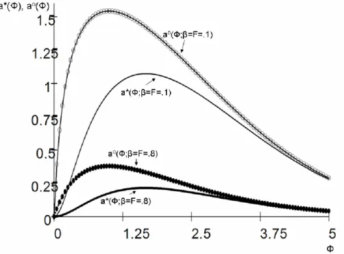
The individual pro…t maximizing and e¢ cient advertising rates for di¤erent market con-centration values are shown in Figure 1 for the di¤erent advertising costs.
16The number of consumers however a¤ect proportionally the equilibrium number of advertisements sent
Figure 1: Individual pro…t maximizing and e¢ cient advertising rates where a ( ; =F =:1) refers to pro…t maximizing advertising rate
under set up and marginal advertising costs being 0:1, etc.
Figure 1 highlights the extent of underadvertising for values of , and illustrates the implications that advertising rates declines with costs. As the market gets to extremes, that is relatively more concentrated and relatively low concentration, equilibrium and e¢ cient rates converge, but the extent of ine¢ cient advertising rate is maximized when = 1.
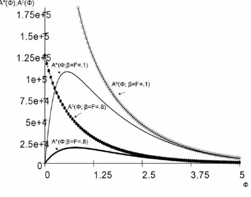
Figure 2: Industry pro…t mazimizing and e¢ cient advertising rates.
The …gure not only highlights the extent of underadvertising at the industry level and how costs a¤ect those rates, but also the result that e¢ cient industry rate is not unimodal in concentration. This implies that the equilibrium industry advertising rate converges to the e¢ cient level only when gets large, and the extent of ine¢ cient advertising rate for the industry is maximized when !0. Finally, Figure 3 shows how costs a¤ect equilibrium and e¢ cient entry, and o. Figure 3 shows that in this model, higher advertising …xed cost increases and o, and hence reduces entry, but also that the di¤erence between and o increases with cost and then decrease again, suggesting that there is an advertising …xed cost value such that the extent of excessive entry reaches a maximum.
ParametersnValues p ( ) a ( ) a ( ) A ( ) A ( ) ( ) =:1; F =:1
= 0:75; = 0:95 0:3472 0:8101 1:5388 101263:64 170980:90 52971:86 59520:52 =:8; F =:8
= 3:70; = 5:10 0:9062 0:0986 0:0381 2664:77 747:65 2537:62 733:58
Table 1: Values for the decentralized market
Figure 3: Equilibrium and e¢ cient levels of entry for di¤erent advertising costs.
Table 1 below shows equilibrium and e¢ cient entry with some associated endogenous variables for di¤erent parameter values of and F, whileN = 100 000.
Before discussing the implications of the numerical example of Table 1, we give an inter-pretation of the numbers. First, set up and marginal costs in the order of 10% of consumers’ valuation (which is 1), induces a free entry concentration level of = 0:75, meaning that
M = 133 333 sellers enter to serve 100 000 consumers, while the e¢ cient level calls for
Mo = 105 263 sellers. Each seller under free entry send s ( ) = N a ( ) = 81010 adver-tisements while e¢ ciency calls for sellers to send s( ) =N a ( ) = 153880 advertisements
each. At the industry level, each consumers receive101263:64advertisement in total from the the 133333 sellers under free entry, while e¢ ciency calls for consumers to receive 170980:9
advertisements from 105263 sellers. The expected number of matches under free entry is found to be 52973. Hence, 52:9% of consumers are satis…ed, and since there are 133333
sellers, only 39:73% make a sale. Under e¢ ciency, nearly 60% of consumers are satis…ed while 56:5% of sellers make a sale.
For set up and marginal costs in the order of 80% of consumers’ valuation, free entry induces a concentration of = 3:7, or M = 27027 sellers enter while the e¢ cient entry calls for a concentration = 5:1, or M = 19607sellers. Each seller under free entry sends
9860 advertisements, while under e¢ ciency each sends3810ads. At the industry level, each consumer receive nearly 2665 ads from all the 27027 sellers under free entry, while under e¢ ciency each consumer receives748 ads only from19607sellers. Finally, from the expected number of matches,2:53%of consumers are satis…ed while9:38%of sellers make a sale under free entry compared to0:73%of satis…ed consumers and3:74%of sellers making a sale under e¢ ciency.
Table 1 highlights the implication that the extent of excessive entry is less important for low costs of advertising. However, as shown in …gure 3, the extent of excessive entry peaks for intermediate values of advertising costs. The interesting features in Table 1 are that the di¤erence between free entry individual and industry advertising rates and e¢ cient ones are reverse going from low to high advertising costs. The same holds for the expected number of matched. For low advertising costs, the free entry equilibrium allocation calls for lower advertising rates than the e¢ cient ones. Therefore one would observe larger number of sellers, each advertising less relative to sellers under e¢ cient entry. However, for high advertising costs, it is reversed. One would observe larger number of sellers, each advertising more relative to sellers under e¢ cient entry. It can be shown that there exists a set of advertising costs such that sellers choose the same advertising rate under free entry equilibrium as sellers under e¢ cient entry. Once again, this example shows that one cannot simply assess e¢ ciency of advertising without considering market concentration.
Finally, we present an example of how the use of a combination of policy instruments can induce free entry to be e¢ cient and yield e¢ cient advertising rate. This is shown in Figure 4 below.