Competitive two-agent scheduling with deteriorating jobs on a single
parallel-batching machine
Lixin Tanga,∗, Xiaoli Zhaoa, Jiyin Liub, Joseph Y.-T. Leungc
a
Liaoning Key Laboratory of Manufacturing System and Logistics, Institute of Industrial Engineering and Logistics Optimization, Northeastern University, Shenyang, 110819, China
b
School of Business and Economics, Loughborough University, Leicestershire LE11 3TU, UK
cSchool of Management, Hefei University of Technology, Hefei, Anhui, 230009, P. R. China and Department of
Computer Science, New Jersey Institute of Technology, Newark, New Jersey 07102, USA
Abstract
We consider a scheduling problem in which the jobs are generated by two agents and have time-dependent proportional-linear deteriorating processing times. The two agents compete for a common single batching machine to process their jobs, and each agent has its own criterion to optimize. The jobs may have identical or different release dates. The batching machine can process several jobs simultaneously as a batch and the processing time of a batch is equal to the longest of the job processing times in the batch. The problem is to determine a schedule for processing the jobs such that the objective of one agent is minimized, while the objective of the other agent is maintained under a fixed value. For the unbounded model, we consider various combinations of regular objectives on the basis of the compatibility of the two agents. For the bounded model, we consider two different objectives for incompatible and compatible agents: minimizing the makespan of one agent subject to an upper bound on the makespan of the other agent and minimizing the number of tardy jobs of one agent subject to an upper bound on the number of tardy jobs of the other agent. We analyze the computational complexity of various problems by either demonstrating that the problem is intractable or providing an efficient exact algorithm for the problem. Moreover, for certain problems that are shown to be intractable, we provide efficient algorithms for certain special cases.
Keywords: Scheduling, Release dates, Agent scheduling, Deterioration, Parallel-batching
∗
Corresponding author. Tel./fax: +86 24 83680169.
E-mail addresses: [email protected] (L. Tang)
1. Introduction
This paper addresses a two-agent scheduling problem on a single batching machine with time-dependent proportional-linear deteriorating job processing times. Each agent has a set of jobs to be scheduled on a common batching machine and seeks to minimize a cost function that only depends on the completion times of its own jobs. The machine can process several jobs simultaneously as a batch. The processing time of a batch is the longest processing time of the jobs assigned to the batch. The processing time of a job is a proportional-linear increasing function of its starting time. The problem we are considering is to find a schedule that minimizes the objective of one agent with the restriction that the objective of the other agent cannot exceed a given bound.
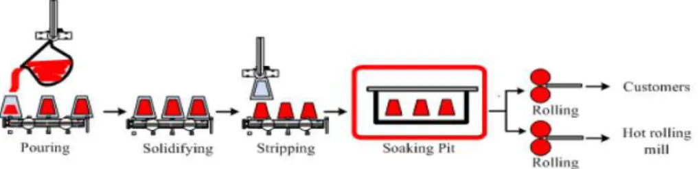
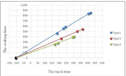
Our study is motivated by a production scheduling problem for the ingot soaking process of a primary rolling plant in the steel industry (see Figure 1). When the molten steel from a steelmaking furnace is ready, it is first cast into ingots. This casting process includes pouring the molten steel into molds, followed by solidifying and stripping to remove the molds. The ingots are then reheated and soaked in a soaking pit to the required rolling temperature before being rolled into steel products, which may be either sold directly to customers or used for further processing in the hot rolling mill. The sales department and the hot rolling mill can be viewed as two agents for the ingot soaking process. An ingot can be viewed as a job. The soaking pit can process several jobs simultaneously and can be considered as a bounded parallel-batching machine. The time required for reheating and soaking an ingot in the soaking pit is known as the soaking time of the ingot. The batch processing time in the soaking pit is the longest soaking times of the jobs assigned to the batch. During the time period between steelmaking and soak-ing, ingots are cast and remain on platforms, which can be moved along rail tracks in the plant. Therefore, this time period is called the track time (Lee, 1979). As the track time increases, the temperature of the ingot decreases, and the required soaking time increases. Depending on the size and shape of the ingot, the increasing rate for the soaking time is different. Patel et al. (1976) provide formulae of the relationship between the soaking time and the track time for three different ingot types. Although the relationship contains a quadratic term, its coefficient is very small, and the relationship is very close to a linear one. Using these relationships and the track times of ingots provided in Lee (1979), ignoring the duplicates and those with track times longer than an eight-hour shift, we calculate the corresponding soaking times and draw the data points in Figure 2. We further fit a line for the points of each ingot type with the restriction that these
three lines must meet at a point on the horizontal axis. The resulting lines are also shown in the figure, which can be clearly observed as a good fit to the points. Note that the starting time of each ingot in the soaking process is the time when the track time ends, e.g., the horizontal coordinate of the corresponding point in Figure 2. As a result, the soaking time of a job can be regarded as a proportional-linear increasing function of its starting time. Consequently, we study a two-agent scheduling problem with time-dependent proportional-linear deteriorating job pro-cessing times on a bounded parallel-batching machine. Moreover, we extend the problems on a bounded batching machine to an unbounded batching machine. For the unbounded model, there is no upper bound on the number of jobs in the same batch. In the following, we will present an example to illustrate the two-agent scheduling model with time-dependent proportional-linear deteriorating job processing times on a bounded parallel-batching machine. In this example, we assume that the hot rolling mill needs 3 steel slabs, which correspond to 3 ingots and can be regarded as the job set of agentA, i.e.,JA={J1A, J2A, J3A}, and customers need 2 steel products, which correspond to 2 ingots and can be regarded as the job set of agentB, i.e.,JB={J1B, J2B}. The actual processing time of job JjX is pXj =αXj (a+bt), X ∈ {A, B}, where αXj > 0 is the normal processing time, a ≥ 0 and b > 0 are constants, and t is the starting time of JjX. In this example, the job normal processing times are α1A= 1, αA2 = 2, αA3 = 3;αB1 = 0.5, αB2 = 1. a=b= 1. The capacity of the soaking pit is 2. We further assume that all jobs have the same release datest0 = 1 and the jobs of different agents cannot be processed in the same batch. The
objective is to minimize the makespanCmaxA of agentA, with the restriction that the makespan
CmaxB of agentB cannot exceed a given boundQB = 32. Introduction of the specific parameters
can be seen in Section 2. We can obtain an optimal schedule π as shown in Figure 3. The minimum makespan of agent A is 15 and the makespan of agent B is 31 < 32. This optimal schedule not only satisfies the customers, but also improves the machine efficiency of the next production stage.
Figure 2. The relationships between the soaking time and the track time
Figure 3. Scheduleπ
Agent scheduling has become a popular topic in the scheduling literature. Baker and Smith (2003) and Agnetis et al. (2004) first introduce the scheduling problems with two agents, in which all jobs have identical release dates. Baker and Smith (2003) consider a linear combination of the objectives of two agents on a single machine, while Agnetis et al. (2004) study the constrained optimization problems and the Pareto-optimization problems on a single machine or in two-machine shop settings. Leung et al. (2010) generalize the results of Agnetis et al. (2004) and extend the models from a single machine to parallel machines, where the jobs are allowed to preempt and have different release dates. For agent scheduling problems, we refer the reader to the recent survey by Perez-Gonzalez and Framinan (2014) and the recent book by Agnetis et al. (2014). Though agent scheduling has been extensively studied in recent years, results of the research focus mainly on agent scheduling with fixed job processing times, see Chapters 3-5 of the book by Agnetis et al. (2014) for details. At the same time, most agent scheduling problems concern jobs with the same release dates on single machine.
The parallel-batching scheduling problems have attracted wide attention in the field of scheduling research. A parallel-batching machine can process several jobs simultaneously. The processing time of a batch is equal to the longest processing time of the jobs in the batch. All the jobs of the same batch start and complete at the same time. Once processing of a batch
begins, it cannot be interrupted, and other jobs cannot be added to the batch. According to the capacity of the batching machine, the problem may be viewed as an unbounded model or a bounded model. Potts and Kovalyov (2000) present a review of scheduling problems with batching.
To the best of our knowledge, there are only two pieces of previous work considering con-strained optimization of two-agent scheduling on a parallel-batching machine, in which the jobs have fixed processing times and the same release dates. Li and Yuan (2012) study the scheduling problems with two agents on an unbounded parallel-batching machine. They provide polyno-mial or pseudo-polynopolyno-mial time algorithms to solve various combinations of regular objective functions for incompatible and compatible agents. Fan et al. (2013) consider the scheduling problems with two agents on a bounded parallel-batching machine. They focus on minimizing the makespan or the total completion time of one agent, subject to an upper bound on the makespan of the other agent for incompatible and compatible agents.
Scheduling problems with time-dependent job processing times have received considerable attention. For these problems, we refer the reader to the survey by Cheng et al. (2004) and the book by Gawiejnowicz (2008). However, the jobs in these time-dependent scheduling works are individual jobs without agents or may be considered as all belonging to one single agent. In this paper, we focus on the scheduling problems with time-dependent proportional-linear deteriorating job processing times and the jobs belonging to two different agents.
Contrary to agent scheduling with fixed job processing times, research on agent scheduling with time-dependent deteriorating job processing times is very limited. Liu and Tang (2008) con-sider the two-agent single machine scheduling problems with proportional deterioration. How-ever, they only focus on the criteria of maximum lateness, makespan, total completion time and maximum cost function. Liu et al. (2010) study the two-agent group scheduling problems with proportional deterioration and proportional-linear deterioration on a single machine. The objective is to minimize the total completion time of the first agent, with the restriction that the maximum cost of the second agent cannot exceed a given upper bound. Gawiejnowicz et al. (2011) consider the two-agent single machine scheduling problem with proportional deteri-oration. The objective is to minimize the total tardiness of the first agent, with the constraint that no tardy job is allowed for the second agent. Gawiejnowicz and Suwalski (2014) first study the two-agent single-machine scheduling problem with proportional deterioration including a non-trivial NP-completeness proof. They propose an exact algorithm and a meta-heuristic for
minimizing a weighted sum of the total weighted completion time of one agent and the maxi-mum lateness of the other agent. Liu et al. (2011) consider two-agent single-machine scheduling problems with proportional-linear deterioration to minimize the objective function of one agent while limiting the objective value of the other agent. They study two problems with different combinations of the objective functions and present optimal polynomial time algorithms to solve them. Yin et al. (2015) extend the research of Liu et al. (2011) to other combinations of the two agents’ objective functions. He and Leung (2016) also consider the two-agent single-machine scheduling problem with proportional-linear deteriorating and proportional-linear shortening job processing times. However, all of the above mentioned works consider only jobs with the same release dates. Agnetis et al. (2014, Section 6.2) provide a detailed discussion of agent scheduling problems with time-dependent deteriorating job processing times.
Although both the two-agent scheduling problems with time-dependent deteriorating job processing times and the implementation of two-agent scheduling problems on a parallel-batching machine have been extensively studied in the literature, we have not identified any previous research reports on an integrated problem with all three features of two-agent, time-dependent deteriorating job processing times and parallel-batching machine altogether. In this paper we study the two-agent scheduling problems on a single parallel-batching machine, in which the processing time of a job is a proportional-linear increasing function of its starting time. Because the single-agent problems and the integrated problems with any of the above two features are only special cases of our problems, our problems are much more complex and more difficult than the previous work on these problems. Because of the deteriorating jobs and the two-agent scheduling in our problems, many solution methods for the previous two-two-agent scheduling problems with fixed job processing times and for the single-agent scheduling problems are no longer suitable for our problems. We exploit the structure of the problem and present optimal properties for different versions of the problem. Based on these properties, we design optimal solutions for the solvable problems. In addition, we show that some problems are NP-hard and develop polynomial or pseudo-polynomial time algorithms to solve certain special cases of these intractable problems. Finally, we generalize the integrated problem to jobs with different release dates. There is no previous result for this scenario even for the version with fixed processing times. We analyze the computational complexity for these problems and establish the foundation of theoretical research for the two-agent scheduling problems with different release dates. For the example case of the ingot soaking problem in the steel industry mentioned earlier, the effective
solution of this integrated scheduling problem can guide the production and save energy in the soaking process, as well as improve customer satisfaction.
The rest of the paper is organized as follows. In Section 2, we specify our notation and provide an overview of the results to be presented in later sections. Section 3 presents the results of the unbounded batching machine scheduling problems. Section 4 discusses the results of the problems on the bounded batching machine. Finally, Section 5 provides conclusions.
2. Notation and overview of problems studied
The problem studied here can be described as follows. There are two agentsAand B. Each of them generates a set of jobs JA = {J1A, J2A, . . . , JnAA} and JB = {J1B, J2B, . . . , JnBB}, respectively. Letnbe the total number of jobs, wheren=nA+nB. The jobs will be processed
nonpreemptively on a common batching machine. The batching machine can process up to
c jobs simultaneously as a batch. We assume that the actual processing time of job JjX is
pXj = αXj (a+bt), X ∈ {A, B}, where αXj > 0 is the normal processing time of job JjX
for j = 1,2, . . . , nX, a ≥ 0 and b > 0 are constants, and t is the starting time of JjX. Let
dXj ≥0 be the due date of job JjX. We assume that either all jobs are simultaneously available for processing at time t0 ≥ 0, or each job JjX has an individual release date rjX > 0. Let
M = (t0 +ab)QnhA=1(1 +αhA)Qnk=1B (1 +αBk)−ab.In a given schedule we denote the completion
time of jobJjX as CjX. We useUjX to indicate whether job JjX is tardy. UjX = 1 , if jobJjX is tardy, andUjX = 0, otherwise.
We consider various scheduling problems denoted by the classification scheme α|β|γA : γB
(Agnetis et al., 2004), where α indicates the scheduling environment, β denotes the additional constraints on the jobs, andγA:γBdefines the objective functionγAof agentAto be minimized subject to the objective function γB of agent B not exceeding a given value QB ≥ 0. In this
paper, we consider one machine problems, implying thatα= 1. Underβ, we usepXj =αXj (a+bt) to indicate the actual processing time of job JjX, j = 1,2, . . . , nX; p−batch represents the
parallel-batching machine;c=∞ and c < nrepresent the unbounded and bounded capacity of the parallel-batching machine, respectively;IF andCF represent incompatible and compatible agents, respectively, where the incompatible agents mean that one batch contains only jobs from the same agent and the compatible agents mean that one batch may contain jobs from different agents;rXj implies that each job has an individual release date and this parameter is omitted if the release dates are equal. We mainly consider the minimization of the following objectives: the
number of tardy jobsP
Uj, the makespanCmax= max{Cj}, the maximum of regular functions
fmax= max{fj(Cj)}, where fj(·) is a nondecreasing function of the completion time of job Jj
and its value can be calculated in constant time for any one job completion time, and the sum of regular functionsP
fj = P
fj(Cj).
3. The unbounded parallel-batching model
In this section, we consider the unbounded parallel-batching scheduling problems. The jobs may have identical or different release dates. We propose algorithms for the problems and show their complexities based on the compatibility of the two agents. Without loss of generality, we assume that the job parameters are non-negative integers.
3.1. The unbounded parallel-batching with identical release dates
We first present the following two properties for the optimal schedules corresponding to different agent compatibility types respectively. The first result characterizes the sequence of jobs of each agent in an optimal schedule for the incompatible agents. The second result characterizes the sequence of jobs of two agents in an optimal schedule for the compatible agents. These properties can be proved by showing that any schedule violating the property can be improved, or at least does not become worse, by shifting jobs to make it satisfy the property. We omit the details of the proof.
Lemma 3.1. There is an optimal schedule for the problem 1|p−batch;pXj = αXj (a+bt);c= ∞;IF|γA :γB, where the jobs (batches) from each agent are processed in the shortest normal processing time (SNPT) order.
We refer to a schedule that satisfies the property in Lemma 3.1 as aD-SNPT-batch schedule. Based on Lemma 3.1, if there are two jobs JiB and JjB with αBi ≤ αBj and dBi ≥ dBj , then the job JiB can be moved to the same batch as the job JjB. Hence, for the problem 1|p−batch;pX
j = αXj (a+bt);c = ∞;IF|γA : fmaxB , we may assume that the jobs of agent B
have been re-indexed such that αB1 < . . . < αBnB and ¯d1B < . . . <d¯BnB, where ¯dBk is an induced deadline and can be calculated in constant time, such that fB
k(CkB) ≤ QB for CkB ≤ d¯Bk and
fkB(CkB)> QB forCkB>d¯Bk.
Lemma 3.2. There is an optimal schedule for the problem 1|p−batch;pX
j = αXj (a+bt);c= ∞;CF|γA:γB, where the jobs (batches) from the two agents are processed in the SNPT order. We refer to a schedule that satisfies the property in Lemma 3.2 as anSNPT-batch schedule.
3.1.1. 1|p−batch;pXj =αXj (a+bt);c=∞|P
fjA:fmaxB
Li and Yuan (2012) propose dynamic programming algorithms for 1|p−batch;c=∞|P
fjA:
fmaxB with fixed processing times for the incompatible and compatible cases. To solve the problems with proportional-linear deteriorating processing times, the running times of these algorithms would be exponential. Hence, in this subsection, we present new dynamic pro-gramming algorithms for the problem based on the compatibility of two agents. Let ∆ = max{fj(M) : 1≤j≤n}. For the incompatible case, we propose the following algorithm with
overall time complexity ofO(n3
AnBn2∆2).
Algorithm DP1
Based on Lemma 3.1, we may assume that the jobs of each agent are indexed according to the SNPT rule, i.e., αA1 ≤αA2 . . .≤ αnAA and αB1 ≤αB2 . . .≤ αBnB. Define C(hA, kB, tA) as the
minimum completion time of a partialD-SNPT-batchschedule containing jobsJA
1 , J2A, . . . , JhAA,
J1B, J2B, . . . , JkB
B such that the objective value of agent A is exactly tA and no job of agent B
completes after its induced deadline. If there is no feasible schedule, we defineC(hA,kB, tA) =
+∞.The initial condition isC(0,0, tA) = t0, iftA= 0, +∞, otherwise.
In a feasible schedule, assume that the last batch comes from agent A and is of the form
JA lA, . . . , J
A
hA with 1≤lA≤hA. Then we haveC(hA, kB, tA) = (1+bα
A hA)C(lA−1, kB, t ∗ A)+aαAhA, wheret∗A=tA− hA P i=lA
fiA(C(hA, kB, tA)). Assume that the last batch comes from agentB and is
of the form JlB B, . . . , J B kB with 1≤lB ≤kB. If (1 +bα B kB)C(hA, lB−1, tA) +aα B kB ≤ ¯ dBl B,where ¯ dBl
B is the induced deadline such that f
B lB((1 +bα B kB)C(hA, lB−1, tA) +aα B kB) ≤ QB, then we haveC(hA, kB, tA) = (1 +bαBkB)C(hA, lB−1, tA) +aα B kB.
Summarizing the above analysis, we have the following recursive relation:
C(hA, kB, tA) = min (1 +bαAh A)1≤minl A≤hA min t∗A∈ΓC(lA−1, kB, t ∗ A) +aαAhA, (1 +bαBk B)1≤minl B≤kB C(hA, lB−1, tA) +aαBkB, if (1 +bαBk B)C(hA, lB−1, tA) +aα B kB ≤ ¯ dBl B. where Γ ={t∗A:t∗A+ hA P i=lA fiA((1 +bαAh A)C(lA−1, kB, t ∗ A) +aαAhA) =tA}.
The value of tA belongs to [0, n∆]. There are nAnBn∆ states in the dynamic program. In
each recursion, the value oft∗Ahas at most n∆ choices, and for eacht∗A, we needO(nA) time to
The optimal solution value is min{tA∈[0, n∆] :C(nA, nB, tA)<+∞}.
Theorem 3.1.1. The problem 1|p−batch;pXj = αjX(a+bt);c = ∞;IF|P
fjA :fmaxB can be solved inO(n3AnBn2∆2) time.
For the compatible case, we propose the following algorithm for the problem 1|p−batch;pXj =
αX j (a+bt);c=∞;CF| P fA j :fmaxB . Algorithm DP2
Based on Lemma 3.2, we may assume that the jobs of two agents are indexed according to the SNPT rule, i.e.,α1 ≤α2 ≤ · · · ≤αn. Define C(j, tA) as the minimum completion time of a
partialSNPT-batchschedule containing jobsJ1, J2, . . . , Jj such that the objective value of agent
Ais exactlytAand no job of agentB completes after its induced deadline. If there is no feasible
schedule, we defineC(j, tA) = +∞.The initial condition isC(0, tA) = t0, iftA= 0, +∞, otherwise.
In a feasible schedule, assume that the last batch is of the form Ji, . . . , Jj with 1 ≤ i≤ j.
Then we have recursive relation:
C(j, tA) = (1 +bαj) min 1≤i≤jtmin∗ A∈Γ C(i−1, t∗A) +aαj, where Γ ={t∗A:t∗A+ j P l=i fl((1 +bαj)C(i−1, t∗A) +aαj) =tA}, fl((1+bαj)C(i−1, t∗A)+aαj) = fl((1 +bαj)C(i−1, tA∗) +aαj), ifJl ∈JA, 0, ifJl∈JB and (1 +bαj)C(i−1, t∗A) +aαj ≤d¯Bl , +∞, ifJl∈JB and (1 +bαj)C(i−1, t∗A) +aαj >d¯Bl .
where ¯dBl is the induced deadline such thatfl((1 +bαj)C(i−1, t∗A) +aαj)≤QB ifJl ∈JB.
The optimal solution value is min{tA∈[0, n∆] :C(n, tA)<+∞}.
Theorem 3.1.2. The problem 1|p−batch;pXj =αjX(a+bt);c =∞;CF|P
fjA : fmaxB can be solved inO(n5∆2) time. 3.1.2. 1|p−batch;pX j =αXj (a+bt);c=∞| P fA j : P fB j
In this subsection, we consider another problem 1|p−batch;pX
j =αXj (a+bt);c=∞| P
fA j : P
fjBbased on the compatibility. We also propose new dynamic programming algorithms for the incompatible and compatible cases. Their computational complexities areO(nAnBn∆QB(n2An∆+
Algorithm DP3
Based on Lemma 3.1, we may assume that the jobs of each agent are indexed according to the SNPT rule, i.e.,αA1 ≤αA2 . . .≤αAnA andαB1 ≤αB2 . . .≤αBnB. DefineC(hA, kB, tA, tB) as the
minimum completion time of a partialD-SNPT-batchschedule containing jobsJ1A, J2A, . . . , JhA
A,
JB
1 , J2B, . . . , JkBB such that the objective values of agent A and agent B are exactly tA and tB,
respectively, and tB ≤QB. If there is no feasible schedule, we define C(hA, kB, tA, tB) = +∞.
The initial condition isC(0,0, tA, tB) = t0, iftA= 0 andtB = 0, +∞, otherwise.
Similar to DP1, we have the following recursive relation:
C(hA, kB, tA, tB) = min (1 +bαAh A)1≤minl A≤hA min t∗ A∈Γ C(lA−1, kB, t∗A, tB) +aαAhA, (1 +bαBk B)1≤minl B≤kB min t∗B∈Γ0C(hA, lB−1, tA, t ∗ B) +aαBkB. where Γ ={t∗A:t∗A+ hA P i=lA fiA((1 +bαAh A)C(lA−1, kB, t ∗ A, tB) +aαAhA) =tA}, Γ0 ={t∗B :t∗B+ kB P i=lB fiB((1 +bαBk B)C(hA, lB−1, tA, t ∗ B) +aαBkB) =tB}.
The values of tA and tB belong to [0, n∆] and [0, QB], respectively. There are nAnBn∆QB
states in the dynamic program. In each recursion, the value oft∗Ahas at mostn∆ choices andt∗B
has at mostQB choices, and we needO(nA) andO(nB) times to check whethert∗A∈Γ andt∗B∈
Γ0 or not, respectively. Hence, allC(hA, kB, tA, tB) can be calculated inO(nAnBn∆QB(n2An∆ +
n2
BQB)) time. The optimal solution value is min{tA ∈ [0, n∆] : C(nA, nB, tA, tB) <+∞, tB ≤
QB}.
Theorem 3.1.3. The problem 1|p−batch;pXj =αjX(a+bt);c=∞;IF|P
fjA :P
fjB can be solved inO(nAnBn∆QB(n2An∆ +n2BQB)) time.
Algorithm DP4
Based on Lemma 3.2, we may assume that the jobs of two agents are indexed according to the SNPT rule, i.e., α1 ≤α2 ≤ · · · ≤αn. Define C(j, tA, tB) as the minimum completion time
of a partialSNPT-batchschedule containing jobsJ1, J2, . . . , Jj such that the objective values of
agentA and agent B are exactlytA and tB, respectively, and tB ≤QB. If there is no feasible
schedule, we defineC(j, tA, tB) = +∞.
The initial condition isC(0, tA, tB) = t0, iftA= 0 andtB = 0, +∞, otherwise.
In a feasible schedule, assume that the last batch is of the form Ji, . . . , Jj with 1 ≤ i≤ j.
Then we have recursive relation:
C(j, tA, tB) = (1 +bαj) min 1≤i≤jt∗ min A∈Γ,t∗B∈Γ0 C(i−1, t∗A, t∗B) +aαj, where Γ ={t∗A:t∗A+ j P l=i flA((1 +bαj)C(i−1, t∗A, t∗B) +aαj) =tA, Jl∈JA}, Γ0 ={t∗B :t∗B+ j P l=i flB((1 +bαj)C(i−1, t∗A, t∗B) +aαj) =tB, Jl ∈JB}.
The optimal solution value is min{tA∈[0, n∆] :C(n, tA, tB)<+∞, tB ≤QB}.
Theorem 3.1.4. The problem 1|p−batch;pXj =αjX(a+bt);c=∞;CF|P
fjA :P
fjB can be solved inO(n5∆2Q2
B) time.
3.1.3. 1|p−batch;pXj = αXj (a+bt);c = ∞|fmaxA : fmaxB , 1|p−batch;pjX = αXj (a+bt);c = ∞|P
UjA:P
UjB and 1|p−batch;pXj =αXj (a+bt);c=∞|P
UjA:fmaxB
In this subsection, we generalize the algorithms proposed by Li and Yuan (2012) for their previous problem with fixed processing times to our problems with time-dependent deteriorating job processing times, we can obtain the corresponding extended results for the new problems with time-dependent deteriorating job processing times. Because of space limit, we omit the details here. If the readers want to read more information, please refer to the paper by Li and Yuan (2012).
Remark 1. For each fixed value QA, whether a feasible schedule exists for the incompatible
and compatible cases of decision problem 1|p−batch;pXj =αjX(a+bt);c=∞|LAmax≤QA:fmaxB
can be determined inO(nnAnB) time and O(n3) time, respectively.
Remark 2. The incompatible and compatible cases of problem 1|p−batch;pXj =αXj (a+bt);c= ∞|LAmax:fmaxB can be solved inO(nnAnBlogM) time and O(n3logM) time, respectively.
Remark 3. The incompatible and compatible cases of problem 1|p−batch;pXj =αXj (a+bt);c= ∞|fmaxA : fmaxB can be solved in O(nnAnBlog(QU −QL)) time and O(n3log(QU −QL)) time,
respectively, whereQL= min{fjA(t0) : 1≤j ≤nA} andQU = max{fjA(M) : 1≤j ≤nA}.
Remark 4. The incompatible and compatible cases of problem 1|p−batch;pXj =αXj (a+bt);c= ∞|P
UjA:P
UjB can be solved in O(n2An2Bn2) time and O(n2nAnB) time, respectively.
Remark 5. The incompatible and compatible cases of problem 1|p−batch;pXj =αXj (a+bt);c= ∞|P
3.2. The unbounded parallel-batching with distinct release dates 3.2.1. 1|p−batch;pXj =αXj (a+bt);rjX;c=∞|CmaxA :CmaxB
In this subsection, we show that the problem 1|p−batch;pX
j =αXj (a+bt);rjX;c=∞|CmaxA :
CmaxB can be solved in polynomial time for both incompatible and compatible cases.
3.2.1.1. 1|p−batch;pX
j =αjX(a+bt);rXj ;c=∞;IF|CmaxA :CmaxB .
In this subsection, we propose a polynomial time algorithm for the incompatible case. We first design a polynomial time dynamic programming algorithm to determine whether a feasible schedule exists for the decision problem 1|p−batch;pjX =αXj (a+bt);rXj ;c=∞;IF|CmaxA ≤QA:
CmaxB . The dynamic programming is based on the following properties of an optimal schedule for the problem 1|p−batch;pXj =αjX(a+bt);rXj ;c=∞;IF|CmaxA :CmaxB .
Lemma 3.2.1. For the problem 1|p−batch;pjX =αXj (a+bt);rXj ;c=∞;IF|CmaxA :CmaxB , there is an optimal batch sequenceπ= (B1, B2, . . . , Bm) such that if two jobsJi andJj belong to the
same agent and distinct batches, withJi ∈Bx,Jj ∈By andx < y, then αi > αj.
Corollary 3.2.2. There is an optimal batch sequence π = (B1, B2, . . . , Bm) for the problem
1|p−batch;pXj =αXj (a+bt);rjX;c=∞;IF|CmaxA :CmaxB such that each batchBx of agentAor
B is in the form Bx ={Jj ∈JX :αl≤αj ≤αu} for some numbersl and u.
If two jobsJi and Jj are from the same agent withri ≤rj and αi≤αj, then we can always
putJi in the same batch as Jj without increasing the makespan of each agent. Thus, we can
deleteJi from the job set. Therefore, without loss of generality, we can re-index the jobs of each
agent such thatr1X < r2X <· · ·< rXnX and αX1 > αX2 >· · ·> αXnX forX=A, B.
Based on the above properties, we present the following dynamic programming algorithm to determine whether a feasible schedule exists for the decision problem 1|p− batch;pXj =
αXj (a+bt);rjX;c =∞;IF|CmaxA ≤QA : CmaxB . Then we use this algorithm as a subroutine to
solve the problem 1|p−batch;pXj =αXj (a+bt);rXj ;c=∞;IF|CmaxA :CmaxB . Algorithm DP5
Given any fixedQA>0, definefQA(hA, kB) as the minimum makespan of a partial schedule
containing jobsJ1A, J2A, . . . , JhA
A, J
B
1 , J2B, . . . , JkBB such that the completion time of the last job of
agentAis at mostQAand the completion time of the last job of agentB is at mostQB. If there
is no feasible schedule, we definefQA(hA, kB) = +∞. The initial condition isfQA(0,0) = 0.
In a feasible schedule, assume that the last batch belongs to agent A and it is of the form {JlA
A+1, J
A
lA+2, . . . , J
A
fA = min 0≤lA≤hA−1 {max{fQA(lA, kB), r A hA} ·(1 +bα A lA+1) +aα A lA+1, if max{fQA(lA, kB), r A hA} · (1 +bαAl A+1) +aα A lA+1≤QA}.
Assume that the last batch belongs to agentB and it is of the form{JlB
B+1, J
B
lB+2, . . . , J
B kB}
withlB< kB. Then we have
fB = min 0≤lB≤kB−1 {max{fQA(hA, lB), r B kB} ·(1 +bα B lB+1) +aα B lB+1, if max{fQA(hA, lB), r B kB} · (1 +bαBl B+1) +aα B lB+1≤QB}.
Hence, the recursive relation isfQA(hA, kB) = min{fA, fB}.
In the above recursive relation, iffQA(nA, nB)<+∞, then we can obtain a feasible schedule
for the decision problem 1|p−batch;pX
j = αXj (a+bt);rjX;c = ∞;IF|CmaxA ≤ QA : CmaxB in
O(nAnBn) time.
Theorem 3.2.3. The problem 1|p−batch;pX
j =αXj (a+bt);rjX;c=∞;IF|CmaxA :CmaxB can be
solved inO(nAnBnlog(Q0U−Q0L)) time, whereQ0U and Q0L are upper and lower bounds ofQA,
respectively.
Proof. For eachQA>0, we can use DP5 as a subroutine to find a feasible schedule such that
CmaxA ≤QA and CmaxB ≤QB.Observe that a lower bound for QA is Q0L =F(nA) which is the
optimal value for the single-agent problem 1|p−batch;pj = αj(a+bt);rj;c = ∞|Cmax that
only schedules the jobsJ1A, J2A, . . . , JnA
A and that can be solved using a dynamic programming
algorithm similar to DP1 of Li et al. (2011) in O(n2A) time. An upper bound for QA is
Q0U =F0(nA) which is the optimal value for the problem 1|p−batch;pAj =αAj(a+bt);rAj;c= ∞;F B|CmaxA , whereFB means forbidden interval. Here “FB” refers to the processing intervals for only optimally scheduling the jobsJ1B, J2B, . . . , JnBB for the problem 1|p−batch;pBj =αBj (a+
bt);rBj ;c=∞|CmaxB . ThenF0(nA) can be optimally solved inO(n2B+n2AnB) time on the basis of
the problem 1|p−batch;rj;c=∞;F B|Cmax(Yuan et al., 2008). We can conduct a binary search
in the range [Q0L, Q0U] to determine the optimal value Q∗A = min{QA : fQA(nA, nB) < +∞}.
Hence, the problem 1|p−batch;pXj =αXj (a+bt);rXj ;c=∞;IF|CmaxA :CmaxB can be solved in
O(nAnBnlog(Q0U−Q0L)). 2
3.2.1.2. 1|p−batch;pjX =αjX(a+bt);rXj ;c=∞;CF|CmaxA :CmaxB .
In view of Lemma 3.2.1, we may assume that the jobs have been indexed such that r1 <
· · ·< rn andα1>· · ·> αn. We define a batch as X-pure if this batch contains only the jobs of
agentX, X =A, B. We have the following properties for the compatible case.
Lemma 3.2.4. For the problem 1|p−batch;pjX = αjX(a+bt);rjX;c = ∞;CF|CmaxA : CmaxB , there is an optimal schedule in the form (π1, π2, π3) that has the following properties:
1) the partial schedule π2 contains only all the B-pure batches, π3 contains part of A-pure
batches (if any), andπ1 contains the remaining batches;
2) all the jobs (batches) in the partial schedulesπ1 and π2 are scheduled in decreasing order of
their normal processing times, all the jobs (batches) in the partial schedulesπ1 and π3 are also
scheduled in decreasing order of their normal processing times.
Lemma 3.2.4 implies that each batch contains only consecutive jobs. Algorithm 1
Based on Lemmas 3.2.1 and 3.2.4, we may assume that the jobs have been indexed as follows: JX
1 , . . . , JiX−1, JiA, JiB+1, . . . , JkB, JkA+1, . . . , JnA,X ∈ {A, B}, such that r1 <· · ·< rn and
α1 >· · ·> αn, where the jobJiAis the last job of agentAinπ1, the jobsJiB+1, . . . , JkB belong to
agentB, the jobJB
k is the last job of agentB, the jobsJkA+1, . . . , JnAbelong to agentA. LetF(j)
be the minimum completion time of a partial schedule of jobsJ1X, . . . , JjX, X ∈ {A, B}. Using the solution method for the single-agent problem 1|p−batch;pj = αj(a+bt);rj;c =∞|Cmax,
which takes O(n2) time, we can obtain the minimum completion time F(j) of any one job Jj
j = 1,2, . . . , n for a given schedule sequence. The minimum completion time of job JkB in the partial schedule of jobsJ1X, . . . , JiX−1, JiA, JiB+1, . . . , JkB is denoted byFopt(k).
1) IfFopt(k)≤QB, then we can computeF(k+1), . . . , F(n) for the job sequenceJ1X, . . . , JiX−1, JiA,
JiB+1, . . . , JkB, JkA+1, . . . , JnA,X ∈ {A, B}. This takesO(n2) time. There are two outcomes: (1) We find the first job Jj ∈JA,fork+ 1≤j≤n, such that F(j) > QB. We denote this job
byJj∗, i.e., F(j∗)> QB.
For j = j∗, j∗+ 1, . . . , n, if the last batch in the partial schedule of jobs J1X, . . . , JiX−1, JiA, JiB+1, . . . , JkB, . . . , JjA contains at least one job of agent B, then we compute F(j) as F(j) =
min
j∗−1≤i≤j−1{max {F(i), rj} ·(1 +bαi+1) +aαi+1}. The time taken to compute F(j) is O(nA). Hence, the running time for this case isO(n2A).
If the last batch in the partial schedule of jobs J1X, . . . , JiX−1, JiA, JiB+1, . . . , JkB, . . . , JjA does not contain any one job of agentB, then we computeF(j) as F(j) = min
k≤i≤j−1{max{F(i), rj} ·
(1 +αi+1) +aαi+1}. The time taken to compute F(j) is O(nA). Hence, the running time for
this case is alsoO(n2A).
(2) IfF(j) ≤QB for all k+ 1≤j ≤n, then we move all jobs Jk+1, . . . , Jn to the front of JkB,
computeF(k) and check whetherF(k)≤QB or not. If yes, then we move all jobsJk+1, . . . , Jn
to the front of JkB−1 and continue to check whether F(k) ≤ QB or not. If yes, we keep doing
case, the optimal solution value of agentA isF(n) that can be obtained in O(n2nB) time.
If when all jobs Jk+1, . . . , Jn are moved to the front of JiB+1 and the minimum completion
time of job JkB is still not greater than QB, then the jobs of agent B before the job JiA from
back to front are moved one-by-one to the position behind the job Jn and are processed in
the same sequence of their original positions, i.e., if JX
i−2, JiX−1 ∈ JB, then we have the
sched-ule J1X, . . . , JiX−3, JiA, JkA+1, . . . , JnA, JiX−2, JiX−1, JiB+1, . . . , JkB. And then compute F(k) and check whetherF(k)≤QB or not. If yes, we keep doing this until the last time the minimum
comple-tion time of job JkB is not greater than QB. There are at most nB movements for the jobs of
agentB before the jobJA
i . So the running time for this case is also O(n2nB).
Summarizing the above analysis, the optimal solution value of agentAisF(n). The running time of the algorithm for this case isO(n2n
B).
2) IfFopt(k)> QB, then the jobs of agentAbefore the jobJiB+1from back to front are moved
one-by-one to the position behind the jobJkBand are processed in the same sequence of their original positions, i.e., ifJiX−1∈JA, then we have the scheduleJ1X, . . . , JiX−2, JiB+1, . . . , JkB, JiX−1, JiA, JkA+1, . . . , JnA. And then compute F(k) and check whether F(k) ≤ QB or not. If no, we keep doing
this until the minimum completion time of job JkB is not greater than QB. There are at most
nA movements for the jobs of agent A before the job JiB+1. Hence, in this case we can obtain
the optimal solution valueF(n) of agentA inO(n2nA) time.
3.2.2. 1|p−batch;pXj =αjX(a+bt);rjX;c=∞|P
UjA:P
UjB
Miao et al. (2012) prove that the problem 1|p−batch;pj =αjt;rj;c=∞|Lmax is NP-hard.
Based on this result, it is easy to see that the problem 1|p−batch;pj = αjt;rj;c = ∞|PUj
is also NP-hard. Consider a special case of the problem 1|p−batch;pXj =αjX(a+bt);rXj ;c = ∞|P
UjA:P
UjB wherea= 0 and the upper bound QB of the objective value PUjB for agent
B is sufficiently large such that the jobs of agentB can be processed at the end of the schedule and start after the completion of all the jobs of agent A, while the upper bound restriction is still satisfied. The problem is then equivalent to the single-agent problem (for agent A) 1|p−batch;pj =αjt;rj;c=∞|PUj. Hence, we have the following result.
Theorem 3.2.5. The problem 1|p−batch;pXj = αjX(a+bt);rXj ;c = ∞|P
UjA : P
UjB is NP-hard for both incompatible and compatible cases.
4. The bounded parallel-batching model
In this section, we consider the complexity of the bounded parallel-batching model based on the compatibility of two agents. We can prove that most of the two-agent scheduling prob-lems with deteriorating jobs on a bounded parallel-batching machine are NP-hard. We present optimal solution methods for some solvable special cases.
4.1. The bounded parallel-batching with identical release dates 4.1.1. 1|p−batch;pXj =αXj (a+bt);c < n|CmaxA :CmaxB
We first show that 1|p−batch;pXj = αXj (a+bt);c < n;IF|CmaxA : CmaxB is solvable in polynomial time.
Theorem 4.1.1. The problem 1|p−batch;pXj = αXj (a+bt);c < n;IF|CmaxA : CmaxB can be solved inO(nlogn) time.
Proof. For each agent, we can obtain an optimal solution in O(nlogn) time by the Full Batch Longest Normal Processing Time (FBLNPT) rule, which is similar to the Algorithm FBLDR proposed by Li et al. (2011). Hence, we can decompose the problem 1|p−batch;pXj =
αXj (a+bt);c < n;IF|CmaxA :CmaxB into two independent subproblems for each agent. Then we can obtain an optimal schedule as follows: all the batches of agentA obtained by the FBLNPT rule are processed first, followed by all the batches of agentB obtained by the FBLNPT rule if
CmaxB ≤QB; otherwise all the batches of agentB are processed first, followed by all the batches
of agentA. IfCmaxB > QB in the second schedule, then the problem has no solution. 2
We now show that 1|p−batch;pXj = αjX(a+bt);c < n;CF|CmaxA : CmaxB is NP-hard by a reduction from the Product Partition Problem, which is known to be NP-complete in the strong sense (Ng et al., 2010).
Product Partition (PP) Problem: Given positive integer numbersa1, a2, ..., am,is there a
subsetS0⊂S:={1,2, ..., m} such thatQ
i∈S0ai =Qi∈S\S0ai?
Theorem 4.1.2. The problem 1|p−batch;pXj =αXj (a+bt);c < n;CF|CmaxA :CmaxB is NP-hard even ifc= 2.
Proof. The decision version of the problem 1|p−batch;pXj =αXj (a+bt);c < n;CF|CmaxA :CmaxB
is clearly in NP. Given an instance of the PP problem, Let D = Q
i∈Sai, and H = √
D, we construct an instance of the decision version of our problem as follows:
There arenA= 3m jobs of m types of agentAand nB =m jobs of agent B.
The normal processing times ofA-agent’s jobs and B-agent’s jobs are defined by
αAi1 =H4iai−1, αAi2 =αiA3=
H4i
ai
−1; αiB=H4i−1; f or i= 1,2, . . . , m.
All jobs are simultaneously available at timet0 = 1.
The upper boundQB is defined byQB =H2(m
2+m)+1
.
The threshold value of agentA is defined byQA=H4(m
2+m)+1
.
It can be seen that the above reduction from the strong NP-complete PP problem is poly-nomial with respect to the input problem length. But the magnitude of the resulting prob-lem parameters is not bounded by a polynomial in the length and the magnitude of the PP problem, and so the reduction is not pseudo-polynomial. Consequently we are proving that 1|p−batch;pXj = αXj (a+bt);c < n;CF|CmaxA : CmaxB is NP-hard in ordinary sense. We now show that there is a schedule to this instance of our problem with CmaxA ≤QA and CmaxB ≤QB
if and only if there is a solution to the PP problem.
If Part. Given a subsetS0 ⊆S such thatQ
i∈S0ai =Qi∈S\S0ai, we construct a schedule for the instance as follows: Bi1 ={JiA1, JiB}fori∈S0,Bi2={JiA2, JiB}fori∈S\S0,Bi3={JiA2, JiA3}
fori∈S0,Bi4 ={JiA1, JiA3} for i∈S\S0. The batches are processed according to the following
order: the batches Bi1 are first scheduled for all i ∈ S0, followed by the batches Bi2 for all
i ∈ S\S0, followed by the batches Bi3 for all i ∈ S0, and followed by the batches Bi4 for all
i∈S\S0. It is easy to show thatCmaxA ≤QA and CmaxB ≤QB.
Only If Part. Given a schedule for the instance with CmaxA ≤QA and CmaxB ≤QB, we can
conclude that each batch contains only two jobs of the same type; i.e., for eachi(1≤i≤m), the jobs JiA1, JiA2, JiA3 and JiB are divided into two batches (Similar to Li et al., 2011, we can obtain this conclusion, so we omit the details here). This implies that the number of batches is exactly 2m and the jobs of agent B are assigned to m distinct batches. Since jobs JiA2 and
JiA3 are identical for i = 1, . . . , m, there are only two ways to partition the four jobs of type
iinto two batches, i.e., {JiA1, JiB} and {JiA2, JiA3}, or {JiA2, JiB} and {JiA1, JiA3}. Assume that the jobs JiA1 and JiB are processed in the same batch Bi1 for i ∈ S0, and the jobs JiA2 and JiB are
processed in the same batch Bi2 for i∈ S\S0. The constraint CmaxB ≤QB =H2(m
2+m)+1
can be satisfied only if all the batches of {JiA1, JiB} and {JiA2, JiB} are first scheduled, so we have
Q i∈S0
ai ≤ H. The constraint CmaxA ≤QA = H4(m
2+m)+1
can be satisfied only if Q i∈S\S0 ai ≤H. Note thatQ i∈Sai =D=H2,so we obtain Q i∈S0 ai = Q i∈S\S0
ai =H, which gives a solution to the
4.1.2. 1|p−batch;pXj =αXj (a+bt);c < n|P
UjA:P
UjB
In this subsection, we discuss the complexity of the problem 1|p−batch;pXj =αXj (a+bt);c < n|P
UjA:P
UjB. We will show that this scheduling problem is NP-hard for both incompatible and compatible cases by showing that the single-agent scheduling problem 1|p−batch;pj =
αj(a+bt);c < n|PUj is NP-hard.
Theorem 4.1.3. The problem 1|p−batch;pj = αj(a+bt);c < n|PUj is NP-hard even if
c= 2.
Proof. We prove this by a reduction from the PP problem. Given an instance of PP, we construct an instance of the decision version of our problem as follows:
n = 4m; a = 0; b = 1; αi1 = H4iai −1, αi2 = αi3 = H 4i ai −1; di1 = di2 = di3 = d1 = H4(m2+m)+1;αi4 =H4i−1; di4 =d2=H2(m 2+m)+1 ; for i= 1,2, . . . , m;t0 = 1;c= 2;Q= 0.
By similar arguments as in the proof of Theorem 4.1.2, we can show that there is a schedule for the instance withP
Uj ≤Q if and only if there is a solution to the PP problem. We omit
the details of the proof. 2
Similar to Theorem 3.2.5, we consider a special case of the problem 1|p−batch;pj =αj(a+
bt);c < n|CmaxA : CmaxB where the upper bound QB of the objective value PUjB for agent
B is sufficiently large. This case is equivalent to the single-agent problem 1|p−batch;pj =
αj(a+bt);c < n|PUj. Hence, we have the following result.
Theorem 4.1.4. The problem 1|p−batch;pXj =αXj (a+bt);c < n|P
UjA:P
UjB is NP-hard for both incompatible and compatible cases.
4.2. The bounded parallel-batching with distinct release dates 4.2.1. 1|p−batch;pXj =αXj (a+bt);rjX;c < n|CmaxA :CmaxB
In this subsection, we first prove that the problem 1|p−batch;pXj = αXj (a+bt);rjX;c < n|CmaxA : CmaxB is NP-hard for both incompatible and compatible cases. Then we consider several polynomially solvable cases for incompatible and compatible agents.
Similar to Theorems 3.2.5 and 4.1.4, we can prove that the problem 1|p −batch;pXj =
αjX(a+bt);rXj ;c < n|CmaxA : CmaxB is equivalent to the single-agent problem 1|p−batch;pj =
αj(a+bt);rj;c < n|Cmax when the upper bound QB of the objective value CmaxB for agent B
is sufficiently large. While the problem 1|p−batch;pj =αj(a+bt);rj;c < n|Cmax is ordinary
NP-hard whena= 0 andb= 1 (Li et al., 2011). Hence, we can easily have the following result. Theorem 4.2.1. The problem 1|p−batch;pXj =αXj (a+bt);rXj ;c < n|CmaxA :CmaxB is NP-hard for both incompatible and compatible cases.
4.2.1.1. Scheduling with l distinct normal processing times for agent A and a common release date for agentB.
In this subsection, we present an optimal algorithm for the incompatible scheduling problem in which the jobs of agentAhavel(l≥2) distinct normal processing times and the jobs of agentB
have a common release daterB >0, wherelis a fixed positive integer. Letα
1, α2, . . . , αlbe thel
distinct normal processing times of agentA. We call the jobs of agentAwith normal processing times αi as type i. Let mi be the number of jobs of type i, then we have Pli=1mi =nA. For
ease of exposition, we denote thejth job of typeiasJi,jA and its corresponding release date can be denoted byrA
i,j fori= 1, ..., landj= 1, ..., mi. We can easily obtain the following properties:
Lemma 4.2.2. For the problem 1|p−batch;pXj = αXj (a+bt);rXj ;c < n;IF|CmaxA : CmaxB ,
in which the jobs of agent A have l distinct normal processing times and the jobs of agent B
have a common release date rB > 0, there is an optimal schedule such that all jobs of agent
B are consecutively scheduled at or after time rB, and they follow the FBLNPT rule, i.e., full batch longest normal processing time, and the jobs of the same type belonging to agent A are processed in non-decreasing order of their release dates.
Lemma 4.2.3. For the problem 1|p−batch;pjX = αXj (a+bt);rjX;c < n;IF|CmaxA :CmaxB , in which the jobs of agentAhave ldistinct normal processing times and the jobs of agent B have a common release daterB >0, there is an optimal schedule for the jobs of agent A such that each batch is full with the possible exception of the first batch for the batches containing some jobs of the same type.
Algorithm DP6
According to Lemma 4.2.2, we first index the jobs of the same type of agent A such that
rAi,1 ≤ rAi,2 ≤ · · · ≤ ri,mA
i for i = 1, ..., l. Let f(h1, h2, ..., hl;n1, n2, ..., nl) be the minimum
completion time of A-agent’s jobs that are processed before agent B satisfying the following conditions: (i) we have assigned jobsJi,A1, Ji,A2, ..., Ji,hA
i for each type i= 1, ..., l before agent B;
(ii) the total number of jobs of type i processed before agent B is at most ni for i = 1, ..., l
and 0 ≤ hi ≤ ni ≤ mi; (iii) the last batch contains the last si jobs of type i (i.e. jobs
Ji,hA
i−si+1, ..., J
A
i,hi) and 0≤si ≤hi fori= 1, ..., l; (iv) the size of the last batch is not more than
the capacity constraint, i.e.,Pl
i=1si≤c.
f(h1, h2, ..., hl;n1, n2, ..., nl) = +∞, ifsi >min{c, hi}, +∞, if Pl i=1si >min{c, Pl i=1hi},
+∞, if for somei0, satisfy 0< si0 < hi0 and Pl
i=1si < c.
The recursive relation isf(h1, h2, ..., hl;n1, n2, ..., nl) = min{max{f(h1−s1, h2−s2, ..., hl−
sl;n1, n2, ..., nl), r(h1, h2, ..., hl;n1, n2, ..., nl)}(1+bα(h1, h2, ..., hl;n1, n2, ..., nl))+aα(h1, h2, ..., hl;
n1, n2, ..., nl) : 0≤si ≤hi ≤ni ≤mi,1≤i≤l,1≤ P 1≤i≤l
si ≤c}, wherer(h1, h2, ..., hl;n1, n2, ...,
nl) = max{rAi,hi :si >0,1≤i≤l} and α(h1, h2, ..., hl;n1, n2, ..., nl) = max{αiA:si>0,1≤i≤
l}denote the release date and the normal processing time of the last batch, respectively. The optimal solution value is min{f(m1, m2, ..., ml;n1, n2, ..., nl)}if max{min{f(m1, m2, ...,
ml;n1, n2, ..., nl)}, rB}Q
dnB
c e
k=1 (1 +bαBk) +ab( QdnBc e
k=1 (1 +bαBk)−1)≤QB,whereαBk is the normal
processing time of each batch of agentB according to the FBLNPT rule. If max{min{f(m1, m2, ..., ml;n1, n2, ..., nl)}, rB}Q dnB c e k=1 (1 +bαBk) +ab( QdnBc e k=1 (1 +bαBk)−1)>
QB, then for each value f(n1, n2, ..., nl;n1, n2, ..., nl), satisfying max{min{f(n1, n2, ..., nl;n1,
n2, ..., nl)}, rB}Q
dnB
c e
k=1 (1 +bαBk) +ab( QdnBc e
k=1 (1 +bαBk)−1)≤QB,use the above recursive relation
to compute the minimum completion time ofA-agent’s jobs that are processed after agentB, i.e.,
f0(m1−n1, m2−n2, ..., ml−nl;m1−n1, m2−n2, ..., ml−nl). At this time, the initial condition
isf0(0,0, ...,0;m1−n1, m2−n2, ..., ml−nl) = max{f(n1, n2, ..., nl;n1, n2, ..., nl), rB}Q
dnBc e
k=1 (1 +
bαBk) + ab(QdnBc e
k=1 (1 +bαBk)−1). Hence, the optimal solution value is min{f
0(m
1−n1, m2 −
n2, ..., ml−nl;m1−n1, m2−n2, ..., ml−nl)}.
It is clear that the complexity of the algorithm isO(n2Alcl).
4.2.1.2. Scheduling with agreeable (reversely agreeable) release dates and normal processing times.
In this subsection, we consider the compatible scheduling problem in which all job release dates and normal processing times are agreeable, i.e., ri < rj implies αi ≤ αj, denoted by agr(rj, αj), or the job release dates and normal processing times are reversely agreeable, i.e.,
ri < rj impliesαi ≥αj, denoted by revagr(rj, αj). By using job-interchange argument, we have
the following properties.
Lemma 4.2.4. For both of the problems 1|p − batch;pXj = αjX(a +bt);agr(rj, αj);c <
n;CF|CmaxA : CmaxB and 1|p−batch;pXj = αXj (a+bt);revagr(rj, αj);c < n;CF|CmaxA : CmaxB ,
there is an optimal schedule in the form (π1, π2, π3) that has the following properties:
1) the partial schedule π2 contains only all the B-pure batches, π3 contains part of A-pure
2) all the jobs (batches) in the partial schedulesπ1 andπ2 are scheduled in non-decreasing order
of their release dates, all the jobs (batches) in the partial schedulesπ1 andπ3 are also scheduled
in non-decreasing order of their release dates. Algorithm 2
By Lemma 4.2.4, we may assume that the jobs have been indexed as follows: JX
1 , . . . , JiX−1, JiA,
JiB+1, . . . , JkB, JkA+1, . . . , JnA, X ∈ {A, B}, such that r1 ≤ r2 ≤ · · · ≤ rn. The definition of each
parameter is the same as in Algorithm 1. Define F(j) as the minimum completion time of a partial schedule containing jobsJ1X, . . . , JjX, forX ∈ {A, B}. Using the solution method for the single-agent problem 1|p−batch;pj =αj(a+bt);rj;c < n|Cmaxthat is similar to Algorithm DP2
proposed by Li et al (2011), we can obtain the minimum completion time F(j) of any one job
Jj j = 1,2, . . . , n for a given schedule sequence inO(nc) time. The minimum completion time
of jobJkB in the partial schedule of jobsJ1X, . . . , JiX−1, JiA, JiB+1, . . . , JkB is denoted byFopt(k).
1) IfFopt(k)≤QB, then we can computeF(k+ 1), . . . , F(n) for job sequence J1X, . . . , JiX−1, JiA,
JiB+1, . . . , JkB, JkA+1, . . . , JnA,X ∈ {A, B}. This takesO(nc) time.
(1) We find the first jobJj ∈JA for k+ 1≤j ≤n such that F(j)> QB. We denote this job
byJj∗, i.e., F(j∗)> QB.
For each j =j∗, j∗+ 1, . . . , n, if the last batch in the partial schedule of jobs J1X, . . . , JiX−1, JiA, JiB+1, . . . , JkB, . . . , JjA contains at least one job of agent B, then compute F(j) as F(j) =
min
[j−(j∗−1)−c]++j∗−1≤i≤j−1{max{F(i), rj}(1 + bαj) +aαj} (for the agreeable case) and F(j) = min
[j−(j∗−1)−c]++j∗−1≤i≤j−1 {max{F(i), rj}(1 +bαi+1) +aαi+1} (for the reversely agreeable case), wherex+= max{x,0}. There are at mostnA values forj and each value ofj can be evaluated
inO(c) time. Hence, the running time for this case isO(nAc).
If the last batch in the partial schedule of jobs J1X, . . . , JiX−1, JiA, JiB+1, . . . , JkB, . . . , JjA does not contain any one job of agentB, then computeF(j) asF(j) = min
(j−c)+≤i≤j−1{max{F(i), rj}(1+
bαj) +aαj}(for the agreeable case) and F(j) = min
(j−c)+≤i≤j−1{max{F(i), rj}(1 +bαi+1) +aαi+1}
(for the reversely agreeable case). There are at mostnA possible values for j and each value of
j can be evaluated inO(c) time. Hence, the running time for this case isO(nAc).
(2) IfF(j)≤QB for all k+ 1≤j ≤n, then the analysis is similar to (2) of Algorithm 1. The
running time for this case isO(nnBc).
2) IfFopt(k)> QB, then the analysis is similar to 2) of Algorithm 1. The running time for this
4.2.2. 1|p−batch;pXj =αjX(a+bt);rjX;c < n|P
UjA:P
UjB
By Theorem 4.1.4, the problem 1|p−batch;pXj =αXj (a+bt);c < n|P
UjA:P
UjBis NP-hard, so when the jobs have different release dates, the problem 1|p−batch;pXj =αXj (a+bt);rXj ;c < n|P
UA j :
P
UB
j is also NP-hard for both incompatible and compatible cases. We consider the
complexity of two special cases in both incompatible and compatible cases, respectively. We will show that the problems with agreeable release dates and due dates in both cases are NP-hard. And the problems with agreeable release dates, due dates, and normal processing times in both cases are solvable in polynomial time.
4.2.2.1. Scheduling with agreeable release dates and due dates.
Theorem 4.2.5. The single-agent problem 1|p −batch;pj = αj(a+bt);rj;c < n|PUj is
NP-hard even if the release dates and due dates are agreeable.
Proof. We prove this by a reduction from the 4-Product problem, which is NP-complete in the strong sense (Kononov, 1996).
An instance of the 4-Product problem can be stated as follows:
4-Product (4-P) problem: Given positive rational numbersa1, a2, . . . , a4p and H such that
H15 < ai < H 1 3 fori= 1,2, . . . ,4p and 4p Q i=1
ai =Hp, does there exist a partition of the set X = {1,2, . . . ,4p} intop disjoint subsets X1, X2, . . . , Xp such thatQi∈Xkai=H fork= 1,2, . . . , p?
The decision version of the problem 1|p−batch;pj =αj(a+bt);rj;c < n|PUj is clearly in
NP. Given an instance of the 4-P problem, we construct an instance of the decision version of the single-agent problem as follows:
There aren= 10p jobs. Let a= 0 and b= 1.
The normal processing times are defined by
αj = H−1, j = 1, . . . , p, ab1 2(j−p+1)c −1, j =p+ 1, . . . ,9p, H−1, j = 9p+ 1, . . . ,10p,
The release dates are defined by
rj =t0= 1, for j= 1, . . . ,9p;r9p+i =H2i−1, fori= 1, . . . , p.
The due dates are defined by
dj =H2j,forj= 1, . . . , p;dj =H2p,forj=p+ 1, . . . ,10p.
It can be seen that the above reduction from the strong NP-complete 4-P problem is poly-nomial with respect to the input problem length. But the magnitude of the resulting prob-lem parameters is not bounded by a polynomial in the length and the magnitude of the 4-P problem, and so the reduction is not pseudo-polynomial. Consequently we are proving that 1|p−batch;pj = αj(a+bt);rj;c < n|PUj is NP-hard in ordinary sense. We now show that
there is a schedule to the instance with P
Uj ≤Q if and only if there is a solution to the 4-P
problem.
If Part. Suppose that there are disjoint subsetsX1, X2, . . . , XpwithXk={lk1, lk2, . . . , lk,nk}
andQ
i∈Xkai =H fork= 1,2, . . . , p, where
p P k=1
nk = 4p. Fori= 1, . . . ,4p, we put jobsJp+2i−1
andJp+2i in a batch. Each batch corresponds to an element of the setXk. This batch is denoted
by{Jp+2i−1, Jp+2i} and has normal processing timeai−1. Fori= 1, . . . , p, we put jobsJi and
J9p+i in a batch. This batch is denoted by {Ji, J9p+i} and has normal processing time H−1.
We construct a batch sequence for the instance as follows:
{Jp+2l11−1, Jp+2l11},{Jp+2l12−1, Jp+2l12}, . . . ,{Jp+2l1,n1−1, Jp+2l1,n1},{J1, J9p+1};
{Jp+2l21−1, Jp+2l21},{Jp+2l22−1, Jp+2l22}, . . . ,{Jp+2l2,n2−1, Jp+2l2,n2},{J2, J9p+2};
. . . .
{Jp+2lp1−1, Jp+2lp1},{Jp+2lp2−1, Jp+2lp2}, . . . ,{Jp+2lp,np−1, Jp+2lp,np},{Jp, J10p}.
It is easily verified that this schedule does not have any tardy jobs, i.e. P
Uj ≤Q= 0.
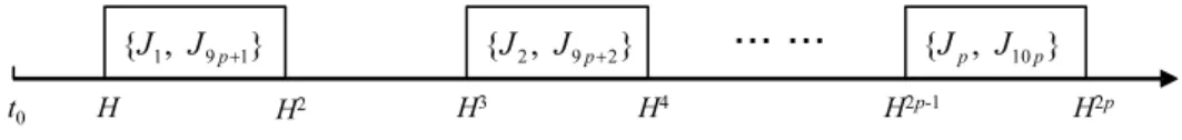
Figure 4. JobsJi, J9p+i(i= 1, . . . , p) in the proof of Theorem 4.2.5.
Only If Part. Given a solution to the instance withP
Uj ≤Q= 0, we can conclude that there
must be no idle time in this schedule and all batches must be full, while the two jobs in each batch must have identical normal processing times. This is because (
10p Q j=1 (1 +αj)) 1 c =H2p = max j {dj}.
In addition, for i = 1, . . . , p, since αi = α9p+i = H −1, ri = t0 = 1, r9p+i = H2i−1 and
di = H2i, jobs Ji and J9p+i must form a batch with starting time H2i−1 and finishing time
H2i (see Figure 4). Thus, all the remaining jobs Jp+j, j = 1, . . . ,8p, must fit into the time
intervals [H2k−2, H2k−1], k = 1,2, . . . , p. Since the two jobs in each batch must have identical normal processing times, we can construct batches as follows: jobsJp+2i−1 andJ2iform a batch,
4p Q h=1 (1 +αAh) = 4p Q h=1
ah = Hp and each of these intervals [H2k−2, H2k−1] has a length of H time
units, the sets of batches within these intervals corresponding to the setsJXk fork= 1,2, . . . , p.
HenceQ
i∈Xkai =H, which gives a solution to the4-Pproblem. 2
By the preceding proof, we can conclude that when the upper bound valueQB of agentB is
sufficiently large, the two-agent scheduling problem is equivalent to the single-agent scheduling problem. Hence, we have the following result.
Theorem 4.2.6. The problem 1|p−batch;pXj = αjX(a+bt);rjX;c < n|P
UjA : P
UjB is NP-hard for both incompatible and compatible cases when the release dates and due dates are agreeable.
4.2.2.2. Scheduling with agreeable release dates, due dates and normal processing times.
We first present a polynomial time algorithm for the incompatible case in which the jobs of each agent have agreeable release dates, due dates and normal processing times, denoted by
agr(rjX, dXj , αjX) for X = A, B. We assume that the jobs of each agent have been re-indexed such that rX1 ≤ · · · ≤ rnXX, dX1 ≤ · · · ≤ dXnX, and αX1 ≤ · · · ≤ αXnX. We have the following property.
Lemma 4.2.7. For the problem 1|p −batch;pjX = αXj (a+bt);rjX;agr(rXj , dXj , αXj ), X =
A, B;c < n;IF|P
UjA :P
UjB, there is an optimal schedule which has the form (E, L), where E is the set of batches containing all the early jobs and L is the set of batches containing all the late jobs. Moreover, all the early jobs that belong to each agent are scheduled in non-decreasing order of their indices and the early batches contain only consecutive jobs.
Algorithm DP7
Define F(hA, uA, kB, uB) as the minimum completion time of the last early batch of a
partial schedule of jobs JA
1 , J2A, . . . , JhAA, J
B
1 , J2B, . . . , JkBB, where the numbers of early jobs of
agentsA and B are at leastuA and uB, respectively. If there is no feasible schedule, we define
F(hA, uA, kB, uB) = +∞. The initial conditions are F(0,0,0,0) = 0; F(hA, uA, kB, uB) = +∞,
ifhA <0 or kB < 0 or uA < 0 or uB < 0. By Lemma 4.2.7, we only consider the early jobs.
When the last scheduled job belongs to agent A: if JA
hA is tardy, then F(hA, uA, kB, uB) =
F(hA−1, uA, kB, uB); if JhAA is early, then based on Lemma 4.2.7, the last early batch will
agentB, we have a similar analysis. Hence, the recursive relation is F(hA, uA, kB, uB) = min min{ min 1≤lA≤min{c,uA} {FlA(hA, uA, kB, uB)}, F(hA−1, uA, kB, uB)}
if the last scheduled job belongs to agentA,
min{ min
1≤lB≤min{c,uB}
{FlB(hA, uA, kB, uB)}, F(hA, uA, kB−1, uB)}
if the last scheduled job belongs to agentB.
where FlA(hA, uA, kB, uB) = max{F(hA−lA, uA−lA, kB, uB), rhAA}(1 +bαAhA) +aαAhA, if max{F(hA−lA, uA−lA, kB, uB), rAhA}(1 +bα A hA) +aα A hA ≤dAh A−lA+1, +∞, otherwise. FlB(hA, uA, kB, uB) = max{F(hA, uA, kB−lB, uB−lB), rkBB}(1 +bαBkB) +aαBkB, if max{F(hA, uA, kB−lB, uB−lB), rBkB}(1 +bα B kB) +aα B kB ≤dB kB−lB+1, +∞, otherwise.
Here, FlA(hA, uA, kB, uB) denotes the completion time of the last early batch of a partial
schedule of jobsJ1A, J2A, . . . , JhA
A, J
B
1 , J2B, . . . , JkBB whenlAjobs (i.e.,J
A hA−lA+1, J A hA−lA+2, . . . , J A hA)
of agent A are processed in the last early batch, and FlB(hA, uA, kB, uB) denotes the
comple-tion time of the last early batch whenlB jobs (i.e.,JkBB−lB+1, J
B
kB−lB+2, . . . , J
B
kB) of agent B are
processed in the last early batch.
The optimal solution value is nA−max{uA|F(nA, uA, nB, uB) <+∞, uB ≥nB−QB,1 ≤
uA≤nA}. The complexity of this algorithm is O(n2An2Bc).
In the following, we present a polynomial time algorithm for the compatible case in which the jobs have agreeable release dates, due dates, and normal processing times, denoted by
agr(rj, dj, αj). We may assume that the jobs have been re-indexed such that r1 ≤ · · · ≤ rn,
d1 ≤ · · · ≤ dn, and α1 ≤ · · · ≤αn. It is easy to see that Lemma 4.2.7 holds for all jobs in this
problem as well. Algorithm DP8
We may assume that the jobs are numbered from J1 toJn according to the EDD sequence.