Total completion time minimization in two-machine flow shop scheduling problems with a fixed job sequence

Total completion time minimization in two-machine flow shop

scheduling problems with a fixed job sequence

F.J. Hwang

a

, M.Y. Kovalyov

b

, B.M.T. Lin

a,∗

a_{Institute of Information Management, Department of Information and Finance Management, National Chiao Tung University, Taiwan}

b_{United Institute of Informatics Problems, National Academy of Sciences of Belarus, Belarus}

a r t i c l e i n f o

Article history:

Received 9 January 2010

Received in revised form 11 November 2011

Accepted 14 November 2011 Available online 6 December 2011

Keywords:

Two-machine flow shop Total completion time Fixed sequence Dynamic programming

a b s t r a c t

This paper addresses schedulingnjobs in a two-machine flow shop to minimize the total completion time, subject to the condition that the jobs are processed in the same given sequence on both machines. A new concept of optimal schedule block is introduced, and polynomial time dynamic programming algorithms employing this concept are derived for two specific problems. In the first problem, the machine-2 processing time of a job is a step increasing function of its waiting time between the machines, and a decision about machine-1 idle time insertion has to be made. This problem is solved inO(n2_)time. In the second problem, the jobs are processed in batches and each batch is preceded by a machine-dependent setup time. AnO(n5_{)algorithm is developed to find an optimal} batching decision.

©2011 Elsevier B.V. All rights reserved.

1. Introduction

This paper studies two scheduling problems in a two-machine flow shop, subject to the condition that the jobs are processed in the same fixed sequence on both machines. A newblock approachis proposed and deployed to determine their solutions in polynomial time within the general dynamic programming framework.

1.1. State of the art

In machine scheduling, a schedule specifies job starting and completion times on the machines. In some cases, it is completely characterized by the job sequence, and in the other cases, extra information is needed to fully specify it. A complicated schedule structure is typical for two major types of scheduling: scheduling with inserted machine idle time [1] and batch scheduling [2]. A commonly used approach to tackle NP-hard problems of these types is to derive an optimal polynomial time algorithm for the problem in which jobs are processed in the same fixed sequence. Then this algorithm can be used in a local search method to evaluate candidate job sequences for the general problem. There also exist studies, in which a specific optimal job sequence is established analytically. In real-life applications, a job sequence can be given as an input data of the problem. Shafransky and Strusevich [3] studied several open shop scheduling problems, subject to a given sequence of jobs on one machine, and mentioned that a pre-assigned sequence of jobs could be retained on one of the machines in the manufacturing process owing to technological or managerial decisions. A fixed job sequence can also appear due to the application of the First-Come–First-Served principle, which is commonly regarded fair by customers.

∗_{Corresponding author. Tel.: +886 3 5131472; fax: +886 3 5723792.}

E-mail addresses:[email protected](F.J. Hwang),[email protected](M.Y. Kovalyov),[email protected],

[email protected](B.M.T. Lin).

1572-5286/$ – see front matter©2011 Elsevier B.V. All rights reserved. doi:10.1016/j.disopt.2011.11.001

Algorithms with machine idle time insertion for a fixed job sequence, also called timing algorithms [4], were applied for a single machine [5–11], parallel machines [12] and a flow shop [13,4]. The problem studied by Lin and Cheng [13] belongs to the area of scheduling with time-dependent processing times, as the machine-2 processing time depends on job’s waiting time between the machines. To avoid extra processing on machine 2, idle times can be inserted on machine 1. Scheduling with time-dependent processing times was surveyed by Cheng et al. [14].

Batching decisions for a fixed job sequence were studied by Cheng et al. [15] and Ng and Kovalyov [16] for the makespan minimization in a flow shop. Considering the fabrication and assembly of components in a two-machine flow shop, Cheng and Wang [17] studied the problem of batching the jobs sequenced according to Johnson’s rule or the agreeable processing time condition for makespan minimization. As for the assembly-type flowshop batching problem with a fixed job sequence, Lin et al. [18] investigated the makespan minimization for the three-machine case. Later, Hwang and Lin [19] addressed the four regular objective functions of total completion time, maximum lateness, total tardiness, and number of tardy jobs for the general

(

m

+

1

)

-machine case. Lin and Cheng [20] also considered the objective of maximum lateness, weighted number of tardy jobs or total weighted completion time for a fixed job sequence with centralized or decentralized batching decisions in concurrent open shops.

In this paper, we consider two problems of total completion time minimization in a two-machine flow shop, subject to a fixed job sequence. Though there exist results for the makespan (Cmax) minimization in these settings, there is no result for the minimization of total completion time, which is one of the most popular and practically relevant criteria in the scheduling literature.

1.2. Formulation of problems and block approach

Denote the processing times of jobjon machine 1 and machine 2 byp1jandp2j, respectively. The first problem includes

a step increasing job processing time on machine 2, which depends on the job waiting time between the machines. We call this waiting time atime lagbetween the two operations of a job. For jobj, it is denoted by

ℓ

jand, given a schedule, it is

equal to the difference between the starting time of this job on machine 2 and its completion time on machine 1. A specified time delaytjis also associated with each jobj. If

ℓ

j

≤

tj, thenp2j

=

α

j; otherwisep2j

=

α

j

+

β

j. Besides the given job

sequence, a schedule should specify machine-1 idle times, which are used to avoid an increase of the job processing times on machine 2, and the time lags between the two operations of each job. Similar to Lin and Cheng [13], who studied the makespan minimization problem in the same setting, our first problem is denoted byF2

|

fixed_seq

,

p2j

∈ {

α

j

, α

j

+

β

j

}|



Cj,

whereF2 stands for a two-machine flow shop,fixed_seqfor a fixed job sequence, and



Cjfor the total completion time

minimization criterion. The problem is motivated by the manufacturing operations in which temperature regime plays a role.

The second problem is to batch jobs in a predefined sequence. The batches are consistent in the sense that their formations are the same on both machines. Job completion times are determined according to the batch availability model such that jobs of the same batch complete on the same machine at the same time, when processing of the last job in this batch has been finished. The processing time of a batchBon machinelis equal to the sum of the machine setup time,sl, and job

processing times,



j∈Bplj. The setups are non-anticipatory, i.e., a setup on machine 2 can start only after the corresponding

batch is completed on machine 1 and machine 2 is unoccupied. Following Ng and Kovalyov [16], we denote this problem by

F2

|

fixed_seq

,

sum-batch

,

consi

,

sl

|



Cj, wheresum-batchstands for the batch processing time calculation formula,consifor

consistent batches, andslfor non-anticipatory machine-dependent setup times. Motivation for this problem comes from

manufacturing environments in which items move between facilities in containers such as pallets, boxes or carts.

In the two problems under study, the difficulty in the design of a polynomial time dynamic programming algorithm stems from the potential conflict between the makespan and the total completion time. A subschedule which minimizes the total completion time for the firstrjobs may retain a relatively large makespan which worsens the total completion time for the remainingn

−

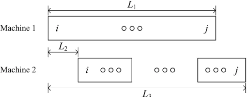
rjobs. To resolve the difficulty that hinders the principle of optimality, a mechanism for fixing the processing lengths of subschedules is required. A common approach is to introduce temporal parameters into the dynamic programs. This however gives rise to pseudo-polynomial running times. This study develops a two-phase dynamic programming framework without including any temporal parameters as state variables. We present a concept that a feasible schedule can be divided into several specific subschedules, each of which is characterized by itsshape. On the Gantt chart, the shape of a subschedule in a two-machine flow shop is determined by the positions of its end on machine 1, its start on machine 2 and its end on machine 2, relative to its start on machine 1.Fig. 1demonstrates that the shape of a subschedule consisting of jobs

{

i

, . . . ,

j

}

is settled by the three-tuple

(

L1

,

L2

,

L3

)

. A specific subschedule is called as ablockand associated with a statein the phase-1 dynamic program. A specific state could be associated with more than one block. These blocks in the same state may have different sums of job completion times, while they must retain an identical shape. Based upon this background idea, the concept ofoptimal(schedule)blockis introduced. The phase-1 dynamic program produces for each state anoptimal block, which is a block attaining the minimum total completion time among all blocks associated with the same state. Then an optimal schedule can be built by concatenating several optimal blocks in the phase-2 dynamic program, which is formulated with backward recursion to establish the validity of the principle of optimality in the studied problems. For the two studied problems, we utilize idle times to divide a feasible schedule into several blocks. Any two consecutive blocks for problems F2

|

fixed_seq

,

p2j

∈ {

α

j

, α

j

+

β

j

}|



CjandF2

|

fixed_seq

,

sum-batch

,

consi

,

sl

|



Cjare separated by

Fig. 1. Illustration for the shape of a subschedule in a two-machine flow shop.

a

b

Fig. 2. Two example schedules.

In Sections2and3, block structures are defined for each problem and then employed in the development of polynomial time dynamic programming algorithms. Without the fixed sequence assumption, the two studied problems are both NP-hard, as will be explained in the corresponding sections. Section4contains a summary of the results and suggestions for future research.

In the sequel, we assume without loss of generality that the fixed job sequence is

⟨

1

,

2

, . . . ,

n

⟩

. 2. ProblemF2

|

fixed_seq

,

p_2j

∈ {

α

j

, α

j

+

β

j

}|



C_j

In many manufacturing environments, it is realistic to consider jobs with time-dependent processing times rather than static and fixed processing times. Lin and Cheng [13] proved the strong NP-hardness of theF2

|

p2j

∈ {

α

j

, α

j

+

β

j

}|

Cmax problem, and designed anO

(

n2

)

_{time solution algorithm for the case with a given job sequence. Minimizing the total} completion time without the assumption of a fixed job sequence is strongly NP-hard because the classicalF2

∥



Cjproblem

corresponds to the special case with

β

j

=

0 ortj

= ∞

for all jobs.

The challenge of problemF2

|

fixed_seq

,

p2j

∈ {

α

j

, α

j

+

β

j

}|



Cjis how to make an optimal decision about the machine-1

idle times to avoid extra processing penalty

β

jon machine 2. Assigning jobs in the given sequence one by one at the earliest

times on the machines and inserting an idle time in front of jobjon machine 1 if the time lag

ℓ

jexceedstjcannot guarantee

an optimal schedule. Consider the following instance with three jobs:

(

p11

,

t1

, α

1

, β

1

)

=

(

1

,

1

,

4

,

1

), (

p12

,

t2

, α

2

, β

2

)

=

(

1

,

1

,

1

,

1

)

, and

(

p13

,

t3

, α

3

, β

3

)

=

(

5

,

1

,

1

,

1

)

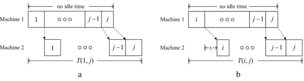
. The total completion time of the schedule obtained by the above-mentioned method is 21 (Fig. 2(a)) while the optimal objective value is 20 (Fig. 2(b)).

For this studied problem, we treat a subschedule in which no machine-1 idle time exists between any two consecutive jobs as a block. An optimal schedule can be either a single block consisting of all jobs

{

1

, . . . ,

n

}

, or a concatenation of several blocks such that there is a machine-1 idle time immediately preceding each block except for the first one. A block is specified as amaximal, by inclusion, subsequence of jobs which are consecutively processed without any idle time between them on machine 1, and characterized by the time lag between the two operations of the first job of this subsequence. The remaining jobs of a block start on machine 2 at the earliest possible times. It is clear that the time lag for job 1 of the first block in an optimal schedule is equal to zero, i.e.

ℓ

1

=

0.

We associate a block consisting of jobs

{

i

, . . . ,

j

}

with the two-tuple

(

i

,

j

)

, and denote its makespan byT

(

i

,

j

)

. The first block

(

1

,

j

),

1

≤

j

≤

n, is illustrated inFig. 3(a). For each block

(

i

,

j

)

with 2

≤

i

≤

j

≤

n, the time lag

ℓ

ihas to be determined.

Lemma 1. Given that schedules comprise at least two blocks for problem F2

|

fixed_seq

,

p2j

∈ {

α

j

, α

j

+

β

j

}|



Cj, there exists an optimal schedule, in which the time lag

ℓ

ibetween the two operations of job i in each block

(

i

,

j

)

is exactly tifor2

≤

i

≤

j

≤

n.

Proof. Assume an optimal schedule where there are block(s) not satisfying the claimed property. Consider the block

(

i

,

j

)

with the smallesti

≥

2. LetIibe the idle time preceding the block

(

i

,

j

)

on machine 1. If

ℓ

i

>

ti, thenp2i

=

α

i

+

β

i. Shift jobi

on machine 1 to the left such that the idle timeIion machine 1 is eliminated. The movement does not increasep2i, and the

a

b

Fig. 3. Structure of (a) the first block(1,j)for 1≤j≤n, and (b) block(i,j)for 2≤i≤j≤n.

Shift jobion machine 1 to the left by min

{

Ii

,

ti

−

ℓ

i

}

time units so that either the idle timeIiis eliminated or the time lag

becomesti. Similarly, the movement does not increasep2i, and the optimality of the schedule remains. In the new schedule,

either block

(

i

,

j

)

vanishes or

ℓ

i

=

tiholds. Repeating the described shifting procedure, whenever necessary, can produce

an optimal schedule as specified in the lemma.

ByLemma 1, we assume that

ℓ

i

=

tifor any block

(

i

,

j

),

2

≤

i

≤

j

≤

n. The structure of block

(

i

,

j

)

for 2

≤

i

≤

j

≤

nis

shown inFig. 3(b).

For problemF2

|

fixed_seq

,

p2j

∈ {

α

j

, α

j

+

β

j

}|



Cj, there exists an optimal schedule which is a single block

(

1

,

n

)

or a

concatenation ofrblocks,

(

1

,

j1

), (

j1

+

1

,

j2

), . . . , (

jr−1

+

1

,

n

)

. Note that each two-tuple

(

i

,

j

)

is associated with only one block, i.e., each block itself is an optimal block. All blocks

(

i

,

j

)

and their corresponding makespan valuesT

(

i

,

j

),

1

≤

i

≤

j

≤

n, can be built by the following pre-processing procedure. To facilitate further presentation, denotep1[i:j]

=



j

h=ip1h. We

haveT

(

1

,

1

)

=

p11

+

α

1, andT

(

i

,

i

)

=

p1i

+

ti

+

α

i

,

2

≤

i

≤

n. For 1

≤

i

<

j

≤

n, T

(

i

,

j

)

=



_T

(

_i

,

_j

−

₁

)

+

α

j

+

β

j

,

ifT

(

i

,

j

−

1

) >

p1[i:j]

+

tj

;

max

{

T

(

i

,

j

−

1

),

p₁[i:j]

} +

α

j

,

otherwise.

In the second phase, we design a backward dynamic programming algorithm, denoted as DP-Idle-Time, in which a single block is added as the prefix of a partial schedule of jobs

{

i

, . . . ,

n

}

. Such a partial schedule is said to be in statei. Algorithm DP-Idle-Time recursively calculates the valueg

(

i

)

, which is the minimum total completion time of the partial schedule(s) in state i

,

1

≤

i

≤

n.Fig. 4illustrates the recursion scenario of algorithm DP-Idle-Time. A dummy job n

+

1 with

p1,n+1

=

tn+1

=

α

n+1

=

β

n+1

=

0 is needed for the boundary condition in algorithm DP-Idle-Time. Denote inequality

T

(

i

,

i′

−

1

) >

p1[i:i′_]

+

t_i′ (1) by condition

A

. Algorithm DP-Idle-Time Initialization: g

(

i

)

=



0

,

ifi

=

n

+

1;

∞

,

otherwise

.

Recursion: (Refer toFig. 4)

For

eachifromndown to 1 do

g

(

i

)

=

min i+1≤i′≤n+1











g

(

i′

)

+

(

n

−

i′

+

1

)(

T

(

i

,

i′

−

1

)

−

p1i′

−

t_i′

)

+

i′−1



h=i T

(

i

,

h

),

if condition

A

;

∞

,

otherwise

.

(2) Goal: Calculateg

(

1

)

.

The optimal objective value isg

(

1

)

and the corresponding optimal schedule can be retrieved by backtracking.

The algorithm is justified as follows. For this problem, we aim to make an optimal decision about which machine-1 operations are to be deferred so that the total completion time is minimized. A crude enumeration requires evaluation of 2n−1_{combinations of decisions on whether to defer each of the jobs}

{

₂

, . . . ,

_n

}

_{. All candidate solutions can be constructed} by the proposed block concatenation. We avoid full enumeration by using algorithm DP-Idle-Time, which in each statei

eliminatesn

−

icandidate partial schedules that are impossible to be extended to constitute an optimal complete schedule. Since the backward recursion is performed, the processing length of the partial schedule in stateiwith valueg

(

i

)

does not affect the remaining unscheduled jobs

{

1

, . . . ,

i

−

1

}

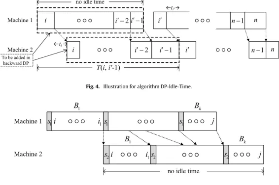
and the optimality of a partial schedule can be kept. In Eq.(2), the optimal values of all possible ‘previous’ statesi′are examined and used to derive the solution of the current statei. As

Fig. 4. Illustration for algorithm DP-Idle-Time.

Fig. 5. Structure of block(i,i1,j,k).

illustrated inFig. 4, condition

A

is employed to guarantee that a partial schedule in stateican be constructed by articulating block

(

i

,

i′

−

₁

)

_{with the partial schedule in statei}′_{which possesses valueg}

(

_i′

)

_{. The ‘min’ operation fori}′_fromi

+

_{1 up ton}

+

₁ in Eq.(2)determines the valueg

(

i

)

, and a partial schedule in stateiwith valueg

(

i

)

dominatesall other partial schedules in the same state. This claim can be proved by induction oni. Denote an arbitrary partial schedule in stateiand its total completion time by

σ

iand

ν(σ

i

)

, respectively. We obviously have the induction baseg

(

n

+

1

)

≤

ν(σ

n+1

)

. The induction hypothesis is that givenj

≤

n

+

1 the inequalityg

(

h

)

≤

ν(σ

_h

)

holds for allh

∈ {

j

, . . . ,

n

+

1

}

. Then we prove thatg

(

j

−

1

)

≤

ν(σ

_j−1

)

. For somej′withj

≤

j′

≤

n

+

1, we assume that there exists a partial schedule

σ

j−1with a leading block

(

j

−

1

,

j′

−

1

)

such that

ν(σ

j−1

) <

g

(

j

−

1

)

. Then we have

ν(σ

j−1

)

=



j

′₋₁

h=j−1T

(

j

−

1

,

h

)

+

(

n

−

j

′

+

₁

)(

_T

(

_j

−

₁

,

_j′

−

₁

)

−

_p

1j′

−

t_j′

)

+

X, whereXis the

total completion time of the partial schedule in statej′_{from which}

σ

j−1is built. From the induction hypothesisX

≥

g

(

j′

)

, it follows that

ν(σ

j−1

)

≥



j′−1

h=j−1T

(

j

−

1

,

h

)

+

(

n

−

j

′

+

₁

)(

_T

(

_j

−

₁

,

_j′

−

₁

)

−

_p

1j′

−

t_j′

)

+

g

(

j′

)

≥

g

(

j

−

1

)

, where the last

inequality is due to Eq.(2). A contradiction arises. We establishg

(

h

)

≤

ν(σ

_h

)

for 1

≤

h

≤

nby induction, and the claim is proved. Hence, the principle of optimality holds and algorithm DP-Idle-Time can generate an optimal solution. An optimal schedule is the schedule in statei

=

1 with valueg

(

1

)

, which is either a concatenation of the first block

(

1

,

i′

−

1

)

and a partial schedule in statei′with valueg

(

i′

)

for 2

≤

i′

≤

n, or the single block

(

1

,

n

)

.

As for the required running time, it is not hard to see that computingT

(

i

,

j

)

for 1

≤

i

≤

j

≤

nrequiresO

(

n2

)

_{time, and} computing the valueg

(

i

)

requiresO

(

n

)

time for eachi. Hence, the running time of algorithm DP-Idle-Time isO

(

n2

)

. Our discussion is summarized in the following theorem. A numerical example is given inAppendix Afor illustration.

Theorem 1.Problem F2

|

fixed_seq

,

p2j

∈ {

α

j

, α

j

+

β

j

}|



Cjcan be solved in O

(

n2

)

time.

3. ProblemF2

|

fixed_seq

,

sum-batch

,

consi

,

sl

|



Cj TheF2

|

sum-batch

,

consi

,

sl

|



Cjproblem is also strongly NP-hard because it is equivalent to the classical problem F2

∥



Cjif setup times are equal to zero. TheF2

|

sum-batch

,

consi

,

sl

|

Cmaxproblem was studied by Cheng et al. [15], Glass et al. [21] and Kovalyov et al. [22]. NP-hardness proofs, polynomial time algorithms for special cases and heuristics were presented in these studies. For the case of a fixed job sequence, Cheng et al. [15] developed anO

(

n3

)

_{algorithm, and Ng and} Kovalyov [16] designed anO

(

n5m−7

)

dynamic programming algorithm if there arem

(

m

≥

2

)

machines.

For problemF2

|

fixed_seq

,

sum-batch

,

consi

,

sl

|



Cj, we define a block as a subschedule associated with a state

(

i

,

i1

,

j

,

k

)

, whereiandjare the first and the last jobs of the block, respectively,kis the number of batches in the block, andi1is the last job of the first batch in the block. It is assumed that the first batch of the block iscriticalin the sense that, for this block, no idle time exists on machine 2 between the completion of the first batch on machine 1 and the completion of the last batch on machine 2. The structure of a block

(

i

,

i1

,

j

,

k

)

is shown inFig. 5.

Fig. 6. Illustration for calculation off(i,i1,j,k).

Notice that a state can be associated with one or more blocks. Letf

(

i

,

i1

,

j

,

k

)

denote the minimum total completion time of jobs in a block among all blocks associated with the same state

(

i

,

i1

,

j

,

k

)

. A block with valuef

(

i

,

i1

,

j

,

k

)

is an optimal block in state

(

i

,

i1

,

j

,

k

)

. Denotepl[i:j]

=



j

h=iplhforl

=

1

,

2, and denote relation

(

k

−

1

)

s1

+

p1[i1+1:j]

≤

(

k

−

1

)

s2

+

p2[i:j′] (3)

by condition

B

. The phase-1 dynamic program calculates valuesf

(

i

,

i1

,

j

,

k

)

for 1

≤

i

≤

i1

≤

j

≤

nand 1

≤

k

≤

j

−

i1

+

1 by forward recursion.

Forward recursion forf

(

i

,

i1

,

j

,

k

)

Initialization:

f

(

i

,

i1

,

j

,

k

)

=



(

i₁

−

i

+

1

)(

s₁

+

p₁[i:i1]

+

s2

+

p2[i:i1]

),

ifj

=

i1, andk

=

1

;

∞

,

otherwise

.

Recursion: (Refer toFig. 6)

For

each feasiblei

,

i1

,

j

,

ksatisfying 1

≤

i

≤

i1

≤

n

−

1

,

i1

+

1

≤

j

≤

n

,

2

≤

k

≤

j

−

i1

+

1 do f

(

i

,

i1

,

j

,

k

)

=

min

i1+k−2≤j′≤j−1



f

(

i

,

i1

,

j′

,

k

−

1

)

+

(

j

−

j′

)(

s1

+

p1[i:i1]

+

ks2

+

p2[i:j]

),

if condition

B

;

∞

,

otherwise. (4)

In the second phase, we construct an optimal schedule by concatenating several optimal blocks. In the following backward dynamic programming algorithm, named as DP-Batch, an optimal block is added as the prefix of a partial schedule of jobs

{

i

, . . . ,

n

}

in state

(

i

,

i1

)

, whereiandi1are respectively the first and the last jobs of the first batch in the partial schedule. The corresponding minimum total completion time is denoted byg

(

i

,

i1

)

. Algorithm DP-Batch recursively calculates valuesg

(

i

,

i1

),

1

≤

i

≤

i1

≤

n. A dummy jobn

+

1 withp1,n+1

= ∞

andp2,n+1

=

0 is used for the boundary condition. Denote relations

i1

+

1

≤

i′

≤

n

+

1

,

i′

≤

i′1

≤

n

+



i′ n

+

1



,

2

−



i1

+

1 i′



≤

k

≤

i′

−

i1 (5)

by range

C

, and denote inequality

ks1

+

p1[i1+1:i1′]

>

ks2

+

p2[i:i ′_−1] (6) by condition

D

. Algorithm DP-Batch Initialization: g

(

i

,

i1

)

=



0

,

ifi

=

i1

=

n

+

1;

∞

,

otherwise

.

Recursion: (Refer toFig. 7)

For

each feasiblei

,

i1satisfying 1

≤

i

≤

i1

≤

ndo g

(

i

,

i1

)

=

min

C



g

(

i′

,

i′₁

)

+

(

n

−

i′

+

1

)(

ks1

+

p1[i:i′_−1]

)

+

f

(

i

,

i₁

,

i′

−

1

,

k

),

if condition

D

;

∞

,

otherwise. (7)

Goal: Find min1≤i1≤ng

(

1

,

i1

)

.

The optimal objective value is min1≤i1≤ng

(

1

,

i1

)

and the corresponding optimal schedule can be obtained by

backtracking.

The algorithm is justified as follows. In this problem, a crude enumeration needs to evaluate 2n−1 _{combinations of} decisions on whether to have a machine-dependent setup time inserted in prior to each of the jobs

{

2

, . . . ,

n

}

. We can

generate all candidate solutions by the presented block concatenation. In the phase-1 dynamic program, Eq.(4)examines all possible ‘previous’ states

(

i

,

i1

,

j′

,

k

−

1

)

confined within rangei1

+

k

−

2

≤

j′

≤

j

−

1 to determine the solution of the current state

(

i

,

i1

,

j

,

k

)

. As demonstrated inFig. 6, condition

B

is used to guarantee that a block in state

(

i

,

i1

,

j

,

k

)

can be built by merging an optimal block

(

i

,

i1

,

j′

,

k

−

1

)

with the single batch consisting of jobs

{

j′

+

1

, . . . ,

j

}

. Note that all blocks in the same state

(

i

,

i1

,

j

,

k

)

retain an identical shape. As defined in Eq.(4), the optimal block

(

i

,

i1

,

j

,

k

)

, i.e. block

(

i

,

i1

,

j

,

k

)

with valuef

(

i

,

i1

,

j

,

k

)

,dominatesall other blocks in the same state in the sense that it has the minimum sum of job completion times among those of all blocks in this state. In the second phase, we develop algorithm DP-Batch by Eq.(7). With range

C

, all possible leading optimal blocks

(

i

,

i1

,

i′

−

1

,

k

)

and ‘previous’ states

(

i′

,

i′1

)

from which the current state

(

i

,

i1

)

can be derived are considered. As shown inFig. 7, condition

D

guarantees that a partial schedule in state

(

i

,

i1

)

can be constructed by articulating the optimal block

(

i

,

i1

,

i′

−

1

,

k

)

with the partial schedule in state

(

i′

,

i′1

)

which has the valueg

(

i′

,

_i′

1

)

. The valueg

(

i

,

i1

)

is obtained by performing the ‘min’ operation in Eq.(7), and a partial schedule in state

(

i

,

i1

)

with valueg

(

i

,

i1

)

dominatesall other partial schedules in the same state. This claim can be proved by induction. Denote an arbitrary partial schedule in state

(

i

,

i1

)

and its total completion time by

σ

i,i1and

ν(σ

i,i1

)

, respectively. Obviously,

the induction baseg

(

n

+

1

,

n

+

1

)

≤

ν(σ

_n+1,n+1

)

holds. Assume, as the induction hypothesis, that givenj

≤

nwe have

g

(

h

,

h1

)

≤

ν(σ

h,h1

)

for allhandh1 withj

≤

h

≤

h1

≤

n

+ ⌊

h

n+1

⌋

. Then we prove thatg

(

j

−

1

,

j1

)

≤

ν(σ

j−1,j1

)

for j

−

1

≤

j1

≤

n. Suppose that for somej′andj′1withj1

+

1

≤

j′

≤

j′1

≤

n

+ ⌊

j′

n+1

⌋

there exists a partial schedule

σ

j−1,j1 which is a concatenation of the optimal block

(

j

−

1

,

j1

,

j

′

−

1

,

k

)

and a partial schedule in state

(

j′

,

j′₁

)

such that

ν(σ

j−1,j1

) <

g

(

j

−

1

,

j1

)

. Then we have

ν(σ

j−1,j1

)

=

f

(

j

−

1

,

j1

,

j

′

−

₁

,

_k

)

+

(

_n

−

_j′

+

₁

)(

_ks

1

+

p1[j−1:j′_−1]

)

+

X, whereX

is the total completion time of the partial schedule in state

(

j′

,

_j′

1

)

from which

σ

j−1,j1is built. By the induction hypothesis X

≥

g

(

j′

,

j′₁

)

, we can obtain that

ν(σ

j−1,j1

)

≥

f

(

j

−

1

,

j1

,

j

′

−

1

,

k

)

+

(

n

−

j′

+

1

)(

ks1

+

p1[j−1:j′_−1]

)

+

g

(

j′

,

j′

1

)

≥

g

(

j

−

1

,

j1

)

, where the last inequality follows from Eq.(7). A contradiction arises. By induction,g

(

h

,

h1

)

≤

ν(σ

h,h1

)

for 1

≤

h

≤

h1

≤

n

is thus established. The principle of optimality holds and algorithm DP-Batch can produce an optimal schedule.

The two-phase dynamic programming algorithm consists of the construction of optimal blocks and the concatenation of optimal blocks. Since there areO

(

n4

)

_states

(

_i

,

_i

1

,

j

,

k

)

, each of which requiresO

(

n

)

operations, all the optimal blocks can be constructed inO

(

n5

)

_{time. Since there areO}

(

_n2

)

_states

(

_i

,

_i

1

)

, each of which requiresO

(

n3

)

operations, the valuesg

(

i

,

i1

)

for 1

≤

i

≤

i1

≤

ncan be obtained inO

(

n5

)

time, too. Finally, the calculation of min1≤i1≤ng

(

1

,

i1

)

requiresO

(

n

)

time. Hence,

the running time of algorithm DP-Batch isO

(

n5

)

_{and the following theorem follows. A numerical example is provided in}

Appendix Bfor illustration.

Theorem 2.Problem F2

|

fixed_seq

,

sum-batch

,

consi

,

sl

|



Cjcan be solved in O

(

n5

)

time.

4. Concluding remarks

This paper studied two scheduling problems in two-machine flow shops, in which the jobs are processed in a predetermined sequence on both machines and the objective is to minimize the total completion time. A new concept of optimal block was suggested and utilized to develop polynomial time dynamic programming algorithms. Problems

F2

|

fixed_seq

,

p2j

∈ {

α

j

, α

j

+

β

j

}|



CjandF2

|

fixed_seq

,

sum-batch

,

consi

,

sl

|



Cjwere solved inO

(

n2

)

andO

(

n5

)

times,

respectively.

Possible extensions of our research include the minimization of due date related performance metric, i.e. the maximum lateness, total tardiness or number of tardy jobs, and more general flow shop environments. For example, the generalm -machine flow shop model can be of further interest. Further research on the second studied problem could be conducted by relaxing the restriction of consistent batches since there could exist an optimal schedule in which the batches are not consistent on two machines. Consider an instance with the following processing times and setup times:p11

=

p21

=

1

,

p12

=

p22

=

2

,

s1

=

5, ands2

=

1. In the optimal schedule, jobs 1 and 2 are grouped into the same batch on machine 1 and then processed with individual batches on machine 2. The max-batch model, in which the processing time of a batch is defined as the maximum processing time of the jobs contained in this batch, rather than the sum-batch model can also be considered in the second problem.

Acknowledgments

The authors are grateful to the anonymous reviewers for their constructive comments that have improved earlier versions of this paper. This research was supported in part by the National Science Council of Taiwan under the grants NSC-98-2410-H-009-011-MY2 and NSC-98-2912-I-009-002.

Appendix A. Example of algorithm DP-Idle-Time

Example 1. Consider the following instance withn

=

3

:

(

p11

,

t1

, α

1

, β

1

)

=

(

1

,

1

,

3

,

1

), (

p12

,

t2

, α

2

, β

2

)

=

(

1

,

1

,

1

,

2

)

, and

(

p13

,

t3

, α

3

, β

3

)

=

(

5

,

1

,

1

,

1

)

. The two-phase algorithm is demonstrated as follows. Phase1. (Calculation of T

(

i

,

j

)

) T

(

1

,

1

)

=

1

+

3

=

4; T

(

2

,

2

)

=

1

+

1

+

1

=

3; T

(

3

,

3

)

=

5

+

1

+

1

=

7; T

(

1

,

2

)

=

4

+

1

+

2

=

7; T

(

1

,

3

)

=

max

{

7

,

7

} +

1

=

8; T

(

2

,

3

)

=

max

{

3

,

6

} +

1

=

7.

Phase2. (Algorithm DP-Idle-Time)

Boundary condition:p1,4

=

t4

=

α

4

=

β

4

=

0. Initialization:g

(

4

)

=

0

;

g

(

1

)

=

g

(

2

)

=

g

(

3

)

= ∞

. Recursion: i

=

3 i′

=

4 T

(

3

,

3

)

=

7

>

p1[3:4]

+

t4

=

5 z1

=

g

(

4

)

+

0

+

T

(

3

,

3

)

=

7; g

(

3

)

=

min

{

z1

} =

7. i

=

2 i′

=

₃ T

(

2

,

2

)

=

3

<

p1[2:3]

+

t3

=

7 z1

= ∞

; i′

=

4 T

(

2

,

3

)

=

7

>

p1[2:4]

+

t4

=

6 z2

=

g

(

4

)

+

0

+

3

h=2T

(

2

,

h

)

=

3

+

7

=

10; g

(

2

)

=

min

{

z1

,

z2

} =

10. i

=

1 i′

=

₂ T

(

1

,

1

)

=

4

>

p1[1:2]

+

t2

=

3 z1

=

g

(

2

)

+

(

4

−

2

)(

T

(

1

,

1

)

−

p12

−

t2

)

+

T

(

1

,

1

)

=

10

+

2

(

4

−

1

−

1

)

+

4

=

18; i′

=

₃ T

(

1

,

2

)

=

7

<

p1[1:3]

+

t3

=

8 z2

= ∞

; i′

=

₄ T

(

1

,

3

)

=

8

>

p1[1:4]

+

t4

=

7 z3

=

g

(

4

)

+

0

+

3

h=1T

(

1

,

h

)

=

4

+

7

+

8

=

19; g

(

1

)

=

min

{

z1

,

z2

,

z3

} =

18. Goal:g

(

1

)

=

18.

The corresponding optimal schedule can be constructed by backtracking the recursion, as illustrated inFig. A.1.

Appendix B. Example of algorithm DP-Batch

Example 2. Consider the following instance withn

=

3

:

(

p11

,

p21

)

=

(

1

,

3

), (

p12

,

p22

)

=

(

2

,

1

), (

p13

,

p23

)

=

(

5

,

1

)

, and

Phase1. (Forward recursion for f

(

i

,

i1

,

j

,

k

)

) Initialization: f

(

1

,

1

,

1

,

1

)

=

(

1

−

1

+

1

)(

s1

+

p11

+

s2

+

p21

)

=

7; f

(

1

,

2

,

2

,

1

)

=

(

2

−

1

+

1

)(

s1

+

p1[1:2]

+

s2

+

p2[1:2]

)

=

20; f

(

1

,

3

,

3

,

1

)

=

(

3

−

1

+

1

)(

s1

+

p1[1:3]

+

s2

+

p2[1:3]

)

=

48; f

(

2

,

2

,

2

,

1

)

=

(

2

−

2

+

1

)(

s1

+

p12

+

s2

+

p22

)

=

6; f

(

2

,

3

,

3

,

1

)

=

(

3

−

2

+

1

)(

s1

+

p1[2:3]

+

s2

+

p2[2:3]

)

=

24; f

(

3

,

3

,

3

,

1

)

=

(

3

−

3

+

1

)(

s1

+

p13

+

s2

+

p23

)

=

9; For other values ofi

,

i1

,

j

,

k, we denotef

(

i

,

i1

,

j

,

k

)

= ∞

. Recursion:

(

i

,

i1

,

j

,

k

)

=

(

1

,

1

,

2

,

2

)

j′

=

₁

(

2

−

1

)

s1

+

p12

=

3

< (

2

−

1

)

s2

+

p21

=

5 z1

=

f

(

1

,

1

,

1

,

1

)

+

(

2

−

1

)(

s1

+

p11

+

2s2

+

p2[1:2]

)

=

7

+

(

1

+

1

+

4

+

4

)

=

17. f

(

1

,

1

,

2

,

2

)

=

min

{

z1

} =

17.

(

i

,

i1

,

j

,

k

)

=

(

1

,

1

,

3

,

2

)

j′

=

₁

(

2

−

1

)

s1

+

p1[2:3]

=

8

> (

2

−

1

)

s2

+

p21

=

5 z1

= ∞

. j′

=

₂

(

2

−

1

)

s1

+

p1[2:3]

=

8

> (

2

−

1

)

s2

+

p2[1:2]

=

6 z2

= ∞

. f

(

1

,

1

,

3

,

2

)

=

min

{

z1

,

z2

} = ∞

.

(

i

,

i1

,

j

,

k

)

=

(

1

,

1

,

3

,

3

)

j′

=

₂

(

3

−

1

)

s1

+

p1[2:3]

=

9

> (

3

−

1

)

s2

+

p2[1:2]

=

8 z1

= ∞

. f

(

1

,

1

,

3

,

3

)

=

min

{

z1

} = ∞

.

(

i

,

i1

,

j

,

k

)

=

(

1

,

2

,

3

,

2

)

j′

=

₂

(

2

−

1

)

s1

+

p13

=

6

=

(

2

−

1

)

s2

+

p2[1:2]

=

6 z1

=

f

(

1

,

2

,

2

,

1

)

+

(

3

−

2

)(

s1

+

p1[1:2]

+

2s2

+

p2[1:3]

)

=

20

+

(

1

+

3

+

4

+

5

)

=

33. f

(

1

,

2

,

3

,

2

)

=

min

{

z1

} =

33.

(

i

,

i1

,

j

,

k

)

=

(

2

,

2

,

3

,

2

)

j′

=

₂

(

2

−

1

)

s1

+

p13

=

6

> (

2

−

1

)

s2

+

p22

=

3 z1

= ∞

. f

(

2

,

2

,

3

,

2

)

=

min

{

z1

} = ∞

. Phase2. (Algorithm DP-Batch)

Boundary condition:p14

= ∞;

p24

=

0. Initialization:

g

(

4

,

4

)

=

0;

Recursion:

(

i

,

i1

)

=

(

3

,

3

)

(

i′

,

_i′ 1

,

k

)

=

(

4

,

4

,

1

)

s1

+

p14

= ∞

>

s2

+

p23

=

3 z1

=

g

(

4

,

4

)

+

0

+

f

(

3

,

3

,

3

,

1

)

=

9. g

(

3

,

3

)

=

min

{

z1

} =

9.

(

i

,

i1

)

=

(

2

,

3

)

(

i′

,

_i′ 1

,

k

)

=

(

4

,

4

,

1

)

s1

+

p14

= ∞

>

s2

+

p2[2:3]

=

4 z1

=

g

(

4

,

4

)

+

0

+

f

(

2

,

3

,

3

,

1

)

=

24. g

(

2

,

3

)

=

min

{

z1

} =

24.

(

i

,

i1

)

=

(

2

,

2

)

(

i′

,

i′₁

,

k

)

=

(

4

,

4

,

2

)

2s1

+

p1[3:4]

= ∞

>

2s2

+

p2[2:3]

=

6 z1

=

g

(

4

,

4

)

+

0

+

f

(

2

,

2

,

3

,

2

)

= ∞

.

(

i′

,

i′₁

,

k

)

=

(

3

,

3

,

1

)

s1

+

p13

=

6

>

s2

+

p22

=

3 z2

=

g

(

3

,

3

)

+

(

3

−

3

+

1

)(

s1

+

p12

)

+

f

(

2

,

2

,

2

,

1

)

=

9

+

3

+

6

=

18. g

(

2

,

2

)

=

min

{

z1

,

z2

} =

18.

(

i

,

i1

)

=

(

1

,

3

)

(

i′

,

i′₁

,

k

)

=

(

4

,

4

,

1

)

s1

+

p14

= ∞

>

s2

+

p2[1:3]

=

7 z1

=

g

(

4

,

4

)

+

0

+

f

(

1

,

3

,

3

,

1

)

=

48. g

(

1

,

3

)

=

min

{

z1

} =

48.

(

i

,

i1

)

=

(

1

,

2

)

(

i′

,

_i′ 1

,

k

)

=

(

4

,

4

,

2

)

2s1

+

p1[3:4]

= ∞

>

2s2

+

p2[1:3]

=

9 z1

=

g

(

4

,

4

)

+

0

+

f

(

1

,

2

,

3

,

2

)

=

33.

(

i′

,

_i′ 1

,

k

)

=

(

3

,

3

,

1

)

s1

+

p13

=

6

=

s2

+

p2[1:2]

=

6 z2

= ∞

. g

(

1

,

2

)

=

min

{

z1

,

z2

} =

33.

(

i

,

i1

)

=

(

1

,

1

)

(

i′

,

_i′ 1

,

k

)

=

(

4

,

4

,

3

)

3s1

+

p1[2:4]

= ∞

>

3s2

+

p2[1:3]

=

11 z1

=

g

(

4

,

4

)

+

0

+

f

(

1

,

1

,

3

,

3

)

= ∞

;

(

i′

,

i′₁

,

k

)

=

(

4

,

4

,

2

)

2s1

+

p1[2:4]

= ∞

>

2s2

+

p2[1:3]

=

9 z2

=

g

(

4

,

4

)

+

0

+

f

(

1

,

1

,

3

,

2

)

= ∞

;

(

i′

,

i′₁

,

k

)

=

(

3

,

3

,

2

)

2s1

+

p1[2:3]

=

9

>

2s2

+

p2[1:2]

=

8 z3

=

g

(

3

,

3

)

+

(

3

−

3

+

1

)(

2s1

+

p1[1:2]

)

+

f

(

1

,

1

,

2

,

2

)

=

9

+

5

+

17

=

31;

(

i′

,

i′₁

,

k

)

=

(

2

,

3

,

1

)

s1

+

p1[2:3]

=

8

>

s2

+

p21

=

5 z4

=

g

(

2

,

3

)

+

(

3

−

2

+

1

)(

s1

+

p11

)

+

f

(

1

,

1

,

1

,

1

)

=

24

+

4

+

7

=

35;

(

i′

,

i′₁

,

k

)

=

(

2

,

2

,

1

)

s1

+

p12

=

3

<

s2

+

p21

=

5 z5

= ∞

; g

(

1

,

1

)

=

min

{

z1

,

z2

,

z3

,

z4

,

z5

} =

31. Goal: min1≤i1≤3g

(

1

,

i1

)

=

g

(

1

,

1

)

=

31.

References

[1] J.J. Kanet, V. Sridharan, Scheduling with inserted idle time: problem taxonomy and literature review, Operations Research 48 (1) (2000) 99–110. [2] C.N. Potts, M.Y. Kovalyov, Scheduling with batching: a review, European Journal of Operational Research 120 (2) (2000) 228–249.

[3] Y.M. Shafransky, V.A. Strusevich, The open shop scheduling problem with a given sequence of jobs on one machine, Naval Research Logistics 45 (7) (1998) 705–731.

[4] Y. Hendel, F. Sourd, An improved earliness-tardiness timing algorithm, Computers & Operations Research 34 (10) (2007) 2931–2938.

[5] M.R. Garey, R.E. Tarjan, G.T. Wilfong, One processor scheduling with symmetrical earliness and tardiness penalties, Mathematics of Operations Research 13 (2) (1988) 330–348.

[6] J.S. Davis, J.J. Kanet, Single-machine scheduling with early and tardy completion costs, Naval Research Logistics 40 (1) (1993) 85–101.

[7] W. Szwarc, S.K. Mukhopadhyay, Optimal timing schedules in earliness-tardiness single machine sequencing, Naval Research Logistics 42 (7) (1995) 1109–1114.

[8] F. Sourd, Optimal timing of a sequence of tasks with general completion costs, European Journal of Operational Research 165 (1) (2005) 82–96. [9] Y. Pan, L. Shi, Dual constrained single machine sequencing to minimize total weighted completion time, IEEE Transactions on Automation Science and

Engineering 2 (4) (2005) 344–357.

[10] E.C. Colina, R.C. Quinino, An algorithm for insertion of idle time in the single-machine scheduling problem with convex cost functions, Computers & Operations Research 32 (9) (2005) 2285–2296.

[11] J. Bauman, J. Józefowska, Minimizing the earliness-tardiness costs on a single machine, Computers & Operations Research 33 (11) (2006) 3219–3230. [12] F. Della Croce, M. Trubian, Optimal idle time insertion in early-tardy parallel machines scheduling with precedence constraints, Production Planning

& Control 13 (2) (2002) 133–142.

[13] B.M.T. Lin, T.C.E. Cheng, Two-machine flowshop scheduling with conditional deteriorating second operations, International Transactions in Operational Research 13 (2) (2006) 91–98.

[14] T.C.E. Cheng, Q. Ding, B.M.T. Lin, A concise survey of scheduling with time-dependent processing times, European Journal of Operational Research 152 (1) (2004) 1–13.

[15] T.C.E. Cheng, B.M.T. Lin, A. Toker, Makespan minimization in the two-machine flowshop batch scheduling problem, Naval Research Logistics 47 (2) (2000) 128–144.

[16] C.T. Ng, M.Y. Kovalyov, Batching and scheduling in a multi-machine flow shop, Journal of Scheduling 10 (6) (2007) 353–364.

[17] T.C.E. Cheng, G. Wang, Scheduling the fabrication and assembly of components in a two-machine flowshop, IIE Transactions 31 (2) (1999) 135–143. [18] B.M.T. Lin, T.C.E. Cheng, A.S.C Chou, Scheduling in an assembly-type production chain with batch transfer, Omega 35 (2) (2007) 143–151.

[19] F.J. Hwang, B.M.T. Lin, Two-stage assembly-type flowshop batching problem subject to a fixed job sequence, Journal of the Operational Research Society (2011), in press (doi:10.1057/jors.2011.90).

[20] B.M.T. Lin, T.C.E. Cheng, Scheduling with centralized and decentralized batching policies in concurrent open shops, Naval Research Logistics 58 (1) (2011) 17–27.

[21] C.A. Glass, C.N. Potts, A.V. Strusevich, Scheduling batches with sequential job processing for two-machine flow and open shops, INFORMS Journal on Computing 13 (2) (2001) 120–137.

[22] M.Y. Kovalyov, C.N. Potts, V.A. Strusevich, Batching decisions for assembly production systems, European Journal of Operational Research 157 (3) (2004) 620–642.