Lake Rotokakahi: The kakahi (Hyridella menziesi) in a general framework of lake health.

(1)

http://waikato.researchgateway.ac.nz/

Research Commons at the University of Waikato

Copyright Statement:

The digital copy of this thesis is protected by the Copyright Act 1994 (New Zealand). The thesis may be consulted by you, provided you comply with the provisions of the Act and the following conditions of use:

 Any use you make of these documents or images must be for research or private study purposes only, and you may not make them available to any other person.

 Authors control the copyright of their thesis. You will recognise the author’s right to

be identified as the author of the thesis, and due acknowledgement will be made to the author where appropriate.

 You will obtain the author’s permission before publishing any material from the thesis.

(2)

Lake Rotokakahi: The kakahi

(Hyridella

menziesi)

in a general framework of lake

health.

A thesis

submitted in partial fulfilment

of the requirements for the degree

of

Master of Science in Biological Science

at

The University of Waikato

by

Joseph Butterworth

The University of Waikato 2008

(3)

ii

Abstract

Lake Rotokakahi is a mesotrophic lake located within the Rotorua Lakes District, North Island, New Zealand. Under the legal guardianship of the Tuhourangi and Ngati Tumatawera tribes of Te Arawa it has remained closed to the public since 1948.

Lake Rotokakahi was last monitored regularly in 1996 under the Environment Bay of Plenty (EBOP) water quality monitoring programme with only the lake outlet (Te Wairoa Stream) being monitored since that time. Water quality data collected up to 1996 suggests that there may be degradation of water quality in the lake, as indicated by declining levels of dissolved oxygen in the bottom waters. Lake Rotokakahi steeped in historical significance, as well as having major cultural and recreational values was well known for its abundant resources and as the name suggests, particularly for its massive supply of the freshwater mussel or kakahi (Hyridella menziesi). Freshwater mussel species worldwide are in decline however little is known on factors controlling kakahi abundance and distribution. The overarching objective of this thesis is update water quality data last monitored in Lake Rotokakahi in 1996 while also identifying key environmental variables thought to influence kakahi populations. This objective is underpinned by a number of aims that include:

• Establishment of a 12-13 month water quality programme within Lake Rotokakahi so that data is obtained for comparisons with previous water quality data (pre-1997) to allow assessment of whether there have been water quality changes in the lake.

• Conduct a population survey of the resident kakahi population examining possible environmental factors influencing their populations.

• Present an oral history of Lake Rotokakahi focusing on its historical significance, water quality, and collection of kairoto (food collected form lakes).

(4)

from the 18September 2006 to 14 September 2007 monthly water sampling was carried out at a mid lake station, the lake outflow and inflow for measures of nutrients, phytoplankton, zooplankton and chlorophyll a. Vertical profiles of temperature dissolved oxygen and chlorophyll fluorescence were also taken on various part of Lake Rotokakahi.

A lengthened period of anoxia in the bottom waters during thermal stratification was recorded with increased levels of chlorophyll a in winter and reduced secchi disk depth indicating an increase in phytoplankton biomass. Nutrient concentrations remain moderate relative to historical data. On going water quality monitoring on Lake Rotokakahi is recommended to further evaluate the extent of which water quality change is occurring. This will provide a better understanding of how Lake Rotokakahi can be best managed to further preserve the lake.

On 1 March and 20 April kakahi were sampled at five sites. Large kakahi densities were distributed predominantly in depths above the hypolimnion. Chlorophyll a fluorescence and dissolved oxygen were found to be the best correlates for kakahi density and biomass respectively. Low dissolved oxygen concentrations in the hypolimnion are thought to restrict kakahi distributions to above the thermocline in periods of hypolimnetic anoxia.

(5)

iv

Acknowledgements

Thank you to my supervisor Professor David Hamilton for your support and expertise in everything within this thesis project. Thank you also to Ngaire Phillips from NIWA for offering your expert advice on the kakahi work.

To the team at the CBER, Dennis Trolle, Deniz Ozkundakci, Chris McBride, Dudley Bell, Alex Ring, Lee Laboryie thanks guys for all your help with lab work and data analysis.

To my ‘masters mates’ Matt Prentice, Matt Riceman, Matt Allan, Ray Tana, Brenda Alderige its been an honour.

To Ian Duggan and Wiki Papa thanks for being mentors for your advice and financial support you have arranged for me and others.

I would like to also acknowledge financial assistance from FRST for the Te Tipu Putaiao Maori fellowship, Ngati Whakaue Education Endowment and Environment Bay of Plenty.

Thank you to the Rotokakahi Board of Control for allowing this study to happen. Also to Frank Maika, Don Stafford and Rangipuawhe Maika thank you for sharing your knowledge with me about the lakes.

To my Whanau, thank you for your never ending support and encouragement. Thanks to Mum and Dad, Melissa, Gavin and Matt, Nan B and Nan C.

Thanks to Erina for your help in the final stages of producing this thesis-its been a wild ride.

(6)

List of Figures

1.0 (a) kakahi (Hyridella menziesi) (b) Snapshot of kakahi distribution in Lake Rotokakahi, using an underwater viewing lens (splashcam) 6 2.1 The location of Lake Rotokakahi amongst the Rotorua lakes 10

2.2 Water sampling and CTD cast sites 12

3.1 Kakahi sampling sites in lake Rotokakahi 19

4.1 Temperol variation in temperature 26

4.2. Spatial variation in dissolved oxygen (mg L-1) and

temperature (ºC) along the CTD transect 27

4.3 Spatial variation in fluorescence (µg L-1)

along the CTD transect 28

4.4 Light attenuation coefficient values (k d) recorded at sites 1-8 29

4.5 Chlorophyll a and Secchi disk depth measurements taken

at 0 m, integrated (0-10 m), 15 m, 27 m and at the outflow 30 4.6 Relative composition of phytoplankton phyla at 0 m and 15 m 32 4.7 Composition of phytoplankton phyla taken at 15 m depth 32 4.8 Relative composition (%) and composition (ml-1) of zooplankton

phyla within the integrated sample (1-10 m) 34

4.9 Total and dissolved nutrients from 0 m, integrated (0-10 m), 15 m,

27 m, outflow and the inflow 36

4.91 Temperature observed and modelled data at 0 m (a),

14 m (b) and 26 m (c) 37

4.92 Dissolved oxygen observed and modelled data at 0 m (a),

(10)

5.1 Mean kakahi densities recorded at each depth 41

5.2 Mean biomass recorded at each depth 41

5.3 Mean kakahi condition at depth 43

5.4 Kakahi size relationships with depth 44

(11)

x

List of Tables

2.1 Lake Rotokakahi morphology 11

2.2 Lake Rotokakahi catchment land cover 11

2.3 GPS coordinates of CTD cast locations 1-8 13

3.0 GPS location of kakahi sampling transects 20

3.1 Visual assessment of the sediment at each site 21

4.1 Monthly readings of euphitic depth (Zeu), light extinction

coefficient (Kd) and Secchi disk depth taken at the mid lake

sampling station 30

5.1 Site characteristics where kakahi were sampled 40

5.2 Pearsons's product mementum correlation matrix of kakahi

density, biomass and environmental variables 45

(12)

Introduction

Chapter 1 Introduction

1.1 Introduction

1.1.1 Eutrophication

Eutrophication of freshwaters is an increasingly global environmental issue (Lee et al, 1978; Smith, 2003; Bronmark and Hansson, 2002; Wetzel, 2001; Rast and Thornton, 1996; Sondergaard and Jeppesen, 2007). It is a natural process, occurring as lakes become progressively shallower and more productive over time, eventually filling with sediment and organic matter to become dry land. Natural eutrophication usually occurs over geological time scales however, it is made much more rapid as a result of impacts from human activities (i.e. cultural eutrophication). Excessive nutrient inputs to lakes, particularly phosphorus and nitrogen, can cause nuisance blooms and surface scums of algae, deoxygenation of bottom waters and in more severe cases, fish kills and deoxygenation of the entire water column (Hamilton, 2007). During the 1950s and 1960s many lakes in Northern Hemisphere urban and agricultural areas experienced intense algal blooms, fish kill events and disappearance of submerged macrophytes. Scientists later proposed that phosphorus used in detergents was largely responsible for these problems, and in many cases phased out this source (Schindler, 1974; Bronmark and Hansson, 2002).

Nutrient loading to a lake originates as either a point source, for example direct sewage and septic tank input, or a diffuse non-point source such as fertilizer applications to farmland. No matter whether it is non-point source or point source, both contribute to the nutrient load that either flows out of the lake or accumulates within the bottom sediments. During seasonal anoxic periods, nutrients in the bottom sediments are released, further adding to the nutrient load to the lake. It is the non point sources of pollution to lakes that are most problematic as eliminating this source is somewhat difficult to pinpoint.

(13)

Introduction

2 Nutrients can also seep into aquifers where they can remain for many of years before flowing into a lake. For example nutrient enriched water from various springs and ground water wells within the western Rotorua and northern Okareka catchments were age-dated, with the majority of samples having mean residence times of over 60 years (Institute of Geological and Nuclear Sciences Ltd, 2004). Similarly in the Lake Taupo catchment the average age of groundwater is between 20-75 years in different stream inflows (Hadfied et al, 2001). Extensive pastoral land developments within the Lake Taupo catchment have contributed significant loads of nitrogen to groundwater within the past 35-40 years causing most of the recent water quality degradation in the lake (Vant & Smith, 2002). Therefore water quality deterioration is often the result of landuse activities within the lake catchment that have occurred many years prior. The Rotorua lakes have been undergoing water quality degradation for the past 30-40 years due to increased nutrient loads of nitrogen and phosphorus from pastoral farming, community sewage inputs and internal loading from the bottom sediments of lakes (Parliamentary Commissioner for the Environment, 2006). This has resulted in eutrophication and increased occurrence of nuisance cyanobacterial blooms (Vincent, 1984; Wilding, 2000; Dell, 2004; Scholes, 2004).

Managing lakes that have become degraded through human interference is not easy. Methods used to influence catchment nutrient loads are generally long-term, often expensive and require and involve catchment land use modification and regulation (Hamilton, 2005), that ultimately impact on local communities.

Measures used to reduce nutrient inputs focus predominantly on diversion of nutrient-enriched inflows (Moss, 1998), natural wetlands (Robertson et al 2000), and sewage reticulation, while in-lake measures include application of water column anti-flocculants (MacIntosh, 2007), lake bottom sediment capping to prevent internal nutrient release events (Özkundakci, 2006) and biomanipulation measures such as fish removal (Gulati & van Donk, 2002) with bivalve filter feeders having potential also (Ogilvie & Mitchell, 1995; James et al 1998; Soto & Mena, 1999; Phillips, 2006).

(14)

Introduction

Therefore as the human population grows and with intensification of landuse, freshwaters are becoming increasingly degraded and impacted upon, threatening environmental, historical, recreational and economic values of freshwater bodies. This is particularly true for Lake Taupo and Rotorua Lakes areas in the North Island of New Zealand where lakes provide important recreational, cultural and economic assets but are becoming increasingly eutrophied.

1.2 The role of filter feeding shellfish in regulating water quality

Freshwater bivalve species feed by filtering the water column of suspended algae and detritus. In dense numbers they have been known to effectively reduce phytoplankton densities, leading to improvements in water clarity and have therefore been recognized as a potential biomanipulation tool for lake restoration (Phillips, 2006; Ogilvie and Mitchell, 1995; White, 2000; MacIsaac et al., 1992). In a study by Soto and Mena (1999) on a bio-control for salmon farming eutrophication in Lake Llanquihue (Chile), the freshwater mussel Diplodon chilensis (Hyriidae) reduced chlorophyll a concentrations by two orders of magnitude (from 300 to 3 µg 1-1). Similar results were found by Hwang et al. (2004) who recorded high consumption rates of phytoplankton by Corbicula leana, affecting planktonic and benthic food web structure and function due to preferential feeding on small seston and through nutrient recycling. Hwang et al. (2004) recommend that control of mussel biomass might therefore be an effective tool for management of water quality in shallow eutrophic lakes and reservoirs in Korea.

The zebra mussel (Dreissena polymorpha) is common in European lakes and can reach very high densities. It can have a positive effect on water clarity although it is a highly invasive encrusting species, causing many problems man-made structures and lake ecosystems (Griffiths et al., 1991; Reeders et al., 1993; Madenjian, 1995). In Lake Erie, Canada, densities up to 700,000 m2 have been recorded with an associated increase in water clarity attributable to the high filtering rate and their ability to remove over 90 % of organic matter suspended in

(15)

Introduction

4 the water column (Reeders and Bij De Vaate 1990; Cooley, 1991, Dermott et al., 1993; MacIsaac, 1996).

Similarly more naturally occurring filter feeders can also significantly impact on water quality by reducing phytoplankton biomass. Ogilvie and Mitchell (1995) report that the freshwater mussel (Hyridella menziesi) population in Lake Tuakitoto, South Otago, New Zealand (area of 118ha and mean summer depth 0.7 m) filters a volume of water equal to that of the lake once every 32 hours.

Although the above positive effects on water quality have been recorded by freshwater mussels there is also increasing evidence to suggest that they can to alter nutrient ratios favouring nuisance algae and promoting phytoplankton growth by supplying high amounts of recycled nutrients to the overlying water column. Results from the study of Asmus and Amus (1991) revealed that Mytilus edulis beds reduced the standing stock of phytoplankton biomass in the overlying water column. However ammonia released from the beds, particularly in summer when phytoplankton are nitrogen-limited, could induce higher phytoplankton primary production despite filtering of the water column by the mussel beds. Nuisance freshwater algae such as cyanobacteria can form blooms and produce toxins that are harmful to humans and animals (Hamil, 2001). Surface scums can degrade the aesthetic values of lakes and also cause taste and odour problems in drinking water (Bykova et al., 2006). There is increasing evidence to suggest a relationship linking the presence of freshwater mussels with increases in cyanobacterial bloom formation. One explanation for this relationship is that mussels can selectively feed on algae, favouring green algae removal and rejecting nuisance algae such as Microcystis sp., resulting in dominance of Microcystis (Heath et al., 1995; Vanderploeg et al. 2001). Similarly Bykova et al. (2006) show that for a lake invaded by zebra mussels, the resulting alteration of nutrient ratios promoted a re-emergence of Microcystis blooms.

(16)

Introduction

1.3 The freshwater mussel-kakahi (Hyridella menziesi)

The New Zealand freshwater mussel or kakahi (Hyridella menziesi) is part of the Unionacea: Hyriidae family of freshwater mussels commonly found throughout Australasia (McMicheal, 1957, Walker, 1981). Hyridella menziesi is widely distributed throughout New Zealand in a variety of habitats ranging from small flowing streams to large rivers and lakes (Phillps, 2006). There are three other species found also in New Zealand; Hyridella aucklandica, Cucumrunio websteri and Cucumerunio websteri delli, however, these species not as widespread as H. menziesi.

Kakahi are commonly found within the littoral zone of lakes but can live down to depths of 30 m in oligotrophic conditions and are known to dominant macroinvertebrate community assemblages, forming dense mussel beds in excess of 600 individuals per m-2 (James, 1985, 1987, Weatherhead & James, 2001). Adults generally range in length from 25 to > 100 mm and are long-lived species, sometimes reaching ages >50 years (Grimmond, 1968).

Early life history of unionid mussels (freshwater mussels) includes a parasitic life stage where juveniles attach to a fish host for dispersal (Atkins, 1979; Phillips, 2006). Spawning occurs in summer with the male releasing sperm into the water column. Eggs kept within the female become fertilised as water is taken in by the female. Larvae are subsequently brooded in the mantle cavity of the female where they develop into glochidial larvae approximately 3 mm long and are released in spring (Phillips, 2006). The glochidia then attach to the fish host usually on the pectoral fins, head and gills, using a larval tooth (Atkins, 1979). Kakahi are known to commonly attach to native fish such as eels (Anguila sp.), koaro (Galaxias brevipennis) and giant and common bullies (Gobiomorphis gobioides and G. cotidianus). This parasitic life stage along with general life cycle of the kakahi are relatively unstudied in New Zealand but could be underpinning observations of declines in kakahi populations. Due to reductions in native fish species in New Zeland, Mc Dowall (2002) states that declines in kakahi could be attributable to losses in native fish that host glochidial larvae.

(17)

Introduction

6 Figure 1.1: (a) Kakahi (Hyridella menziesi) (b) Snapshot of kakahi distribution in Lake Rotokakahi, using an underwater viewing lens (splashcam)

1.4 Environmental factors influencing kakahi growth and distribution

There is very little scientific information published on H. menziesi within lakes, and certain knowledge gaps remain in aspects of its life cycle, physiology and factors controlling its abundance and distribution. The use of freshwater mussels as a bioindicator species in environmental studies has been investigated in previous studies (Sanki et al., 2003 Roper & Hickey, 1995; Hickey et al., 1995). Similarly microcystin accumulation in kakahi tissue arising from high levels of cyanobacteria has been quantified in some of the Rotorua lakes (Wood et al., 2006). Kakahi shell abnormalities have been linked to the presence of a chironimid parasite (Forsyth, 1979; Forsyth & McCallum, 1978). James (1985) has studied the environmental factors that regulate distribution, biomass and production of kakahi in Lake Taupo New Zealand. He found through a series of multiple regression analyses that percentage of clean sand and lake bed slope were key environmental variables positively associated with kakahi density. Also, kakahi were found to be most prominent at depths below the macrophyte zone and where sediments are fine and detritus-rich (Weatherhead & James, 2001). However no data exists for potential impacts on kakahi due to a transition to decreased water quality, specifically the sort of declines that have occurred in the Rotorua lakes. It is known that the kakahi can dominate macroinvertebrate biomass in New Zealand lakes, yet there has been only one quantitative study made on the distribution and abundance of kakahi in Lake Taupo (James, 1985).

(18)

Introduction

1.5 Lake Rotokakahi

1.5.1 Historical background

The Iwi of Te Arawa has resided in the Rotorua area for more than 600 years and the lakes of the region were taonga (treasures) for Te Arawa and the foundation of their identity, cultural integrity, wairua, tikanga and kawa. With increasing European settlement around the lakes in the late 1800s, forests were milled, agriculture was established and urban settlements were developed. Numerous conflicts developed between the new settlers and Te Arawa, whose capacity to provide kairoto (food from lakes) from the lakes and koha (gifts) for hospitality was diminished with deteriorating water quality and introductions of exotic species. This culminated in 1922 with the Crown taking ownership of the lakes from Te Arawa in return for a fixed annuity of £6000 paid from the Crown. The only major lake exempt from this arrangement was Rotokakahi (Green Lake). Over the tenure of Crown ownership the Rotorua lakes have become progressively degraded. As a consequence the Te Arawa people have progressively become alienated from the lakes, their taonga (tresures) have been eroded and their role as kaitiaki (gaudians) has been negated. Only in 2004 did the Crown finally agree to offer Te Arawa Maori Trust Board a settlement package for grievances in relation to the lakes.

Lake Rotokakahi is a lake of particular importance to the Te Arawa people and is steeped in historical significance, as well as having major cultural and recreational values. It is currently closed to the public and under legal guardianship of Ngati Tumatawera and Ngati Wahiao/Tuhourangi. A particular concern to the kaitiaki of this lake is its present health, which may be declining, though it has not been studied intensively. Lake Rotokakahi was last monitored regularly in 1996 under the Environment Bay of Plenty (EBOP) water quality monitoring programme, with only the lake outlet (Te Wairoa Stream) being monitored since that time. Baseline monitoring of Lake Rotokakahi was conducted by Jolly (1967) followed by Mc Coll (1972) who determined bottom waters as anoxic for at least 3 months of the year subsequently classing Lake Rotokakahi as mestrophic based on hypolimnion deoxygenation. Data collected by EBOP up to 1996 suggests that there may be degradation of water quality in the lake, as indicated by declining

(19)

Introduction

8 levels of dissolved oxygen in the bottom waters (EBOP 2002). Lake water quality indicated through the trophic level index (TLI) also suggests water quality has degraded from 1990. The Proposed Regional Water and Land Plan (PRWLP) TLI target objective has been exceeded by 0.2 TLI units for two years and as a result a risk assessment has been completed and the lake is ranked fifth out of the seven lakes to undergo prioritization of land management options (EBOP, 2007).

Lake Rotokakahi was well known for its abundant resources and as the name suggests, particularly for its massive supply of the freshwater mussel or kakahi (Hyridella menziesi). The kakahi formed a major component of the Maori people’s diet and was especially important to babies who could suck the kakahi from its shell after it was cooked. It was once said “ko te kakahi te whaea o nga tamariki”, which translates to “the kakahi is the mother of the children”, representing its importance as an appropriate food source for babies and young infants who could easily suckle the flesh of the kakahi similar to taking milk from its mother (Hiroa 1921). Kakahi shells were also used as scraping and cutting tool and for ornamental purposes (Hiroa, 1921).

Environmental factors regulating kakahi populations in lakes may ultimately be very important for water quality and this understanding could be transferred into the Maori community so that they can be pro-active in managing kakahi and actively participating in determining the future of the Rotorua lakes. This thesis presents a preliminary attempt to link environmental factors to kakahi abundance in Lake Rotokakahi and to provide Iwi with the background information that might be useful in helping them to manage, and enhance kaitiakitanga (Gaurdianship) over both the kakahi and the Lake Rotokakahi environment.

1.6 Aims and objectives

The overarching objective of this thesis is update water quality last monitored in Lake Rotokakahi in 1996 while also identifying key environmental variables influencing kakahi populations. These objectives are underpinned by a number of aims that include:

(20)

Introduction

• Establishment of a one-year water quality programme within Lake Rotokakahi so that data is obtained for comparisons with previous water quality data (pre-1997) to allow assessment of whether there have been water quality changes in the lake.

• Conducting a population survey of the resident kakahi population examining possible environmental factors influencing their populations. • Presenting an oral history of Lake Rotokakahi focusing on the its historical

significance, past water quality conditions and collection of kairoto (food collected from the lake).

(21)

Water Quality Methods

10

Chapter 2 Water Quality Methods

2.1 Study site

Lake Rotokakahi is located within the Rotorua lakes District located within the Bay of Plenty, North Island New Zealand. (Fig. 2.1) Fourteen lakes comprise the Rotorua lakes, all of volcanic origin due to their position within a highly active geothermal zone - the Taupo Volcanic Zone. Most lakes have formed through subsidence, infilling of calderas and damning of river valleys. In geological time Lake Rotokakahi is a relatively young lake, forming 13,300 years ago as a result of a damned river valley following various volcanic eruptions (Healy, 1963). The lake is considered mesotrophic (McColl 1972; Environment Bay of Plenty, 2006) has an area of 4.4 km2 and catchment area of 19.7 km2 comprised mainly of exotic forest (57.1 %) (Environment Bay of Plenty, 2006) although current logging operations within the lake catchment would have reduced total exotic forest land cover. It is fed by a small stream and groundwater, with the lake outflow (Te

Lake Rotokakahi

Lake Tikitapu _{Lake Tarawera}

Lake Rotomahana Lake Rotorua Lake Okataina Lake Rotoiti Lake Rotoehu Lake Rotoma Lake Rerewhakaitu Lake Okaro Lake Okareka Lake Rotokawau

(22)

Wairoa Stream) draining the lake at the north eastern end which eventually flows into Lake Tarawera (Environment Bay of Planty, 2006). Table 2.1 and 2.2 summarise Lake Rotokakahi morphology and catchment land cover respectively

2.2 Water quality data collection

2.2.1 Field water sampling

Water quality monitoring was conducted monthly from 18 September 2006 to 14 September 2007. Water samples were collected from a mid lake sampling station and from the lake inflow and outflow (Te Wairoa Stream) (Fig. 2.2). At the mid lake sampling station samples were taken at four selected depths through the water column including the surface (0 m), surface-integrated (I.S.; 0-10 m), 15 m and 28 m depths for subsequent analysis of dissolved and total nutrients and chlorophyll a. The latter two water samples were an attempt to obtain thermocline and near-bottom-water samples. Surface integrated samples, were collected using a 10 m tube sampler, while surface samples were collected by immersing a sample bottle just below the surface. A Schindler-Patellas trap was used to collect samples at 15 and 27 m. From each of these depths unfiltered water samples were taken for total nitrogen and total phosphorus analysis while water samples taken for dissolved nutrients and chlorophyll a were filtered in the field through a 60 mL plastic syringe and Swinnex glass fibre filter. All samples were kept on ice while in the field and then taken back to the laboratory and stored frozen at -20°C

Lake area (km2) Catchment area (km2) Max depth (m) Mean depth (m) Long axis (km) Altitude (m above msl) 4.6 19.7 32 17.5 4.3 394

Catchment land cover (%) Pasture Indigenous

forest/scrub

Urban Exotic forest 26.3 16.6 0 57.1

Table 2.1. Lake Rotokakahi morphology (Environment Bay of Plenty, 2007)

(23)

12 until analysis. Water samples were analysed for total nutrients (total phosphorus TP and total nitrogen TN), dissolved nutrients (soluble reactive phosphorus (PO4

-P), ammonium (NH4-N), nitrate + nitrite (NO3–N + NO2-N), chlorophyll a,

phytoplankton, and zooplankton.

2.2.2 Conductivity-Temperature-Depth (CTD) Profiling

A Conductivity-Temperature-Depth Probe (CTD) (SBE 19 and SEACAT Profiler, Washington) was used to measure conductivity and temperature variations with depth. Additional sensors for dissolved oxygen (Sea-Bird Electronics Inc.) and chlorophyll a fluorescence (Chelsea Instruments Ltd) allowed for profiles to be taken for these variables. CTD profiles were taken at monthly intervals at eight stations on the same day as water sampling. The location of each station was chosen to form a transect along the longest lake axis (Fig 2.2, Table 2.3) in order to construct profiles of the various measurements along the entire lake length using the graphics programme Ocean Data Viewer. The measurements included temperature, dissolved oxygen and chlorophyll a fluorescence with depth.

Figure.2.2 Water sampling and CTD cast sites. = water sampling location, = CTD cast site. 0 1 km N Outflow Mid-lake sampling station Inflow 1 3 2 4 5 6 7 8

(24)

CTD Site Depth (m) GPS co-ordinates 1. 10 38° 13’ 01. 198 S 176° 17’ 56. 457 E 2. 24 38° 13’ 03. 731 S 176° 18’ 17. 587 E 3. 30 38° 13’ 02. 330 S 176° 18’42. 187 E 4. 23 38° 13’ 39. 819 S 176° 18’ 48. 065 E 5. 29 38° 13’ 01.198 S 176° 19’ 05.714 E 6. 22 38° 12’ 50. 177 S 176° 19’ 22. 947 E 7. 22.5 38_{176 18 51. 663 E}° 12’ 39. 325 S 8. 15.7 38 12 26. 433 E 176 20 29. 105 E

2.3 Water Quality Data processing

2.3.1 Light attenuation coefficient (Kd) and euphotic depth (zeu )

The light attenuation coefficient was determined using photosynthetically active radiation (PAR) data collected by the CTD. PAR data was subsequently log10

transformed and entered into the following equation:

z z I I K_d = ln( (0))−ln( ( )) Where:

I(0) = PAR at the surface and the depth where PAR = 0 I(z) = PAR at depth where z = 0

z = depth where I(z) was taken

The euphotic zone depth was estimated as 2.5 x the monthly secchi disk depth reading.

2.3.2 Chlorophyll a analysis

(25)

14 Samples for chlorophyll a analysiswere collected in the field by flushing 100 mL of water sample from each depth (0 m, I.S, 15 m, 28 m) through a 0.45 µm glass fibre filter using a 60 mL syringe and attached filter tip. Filter papers were wrapped in aluminum foil and placed on ice until return to the laboratory where filters were deep-frozen. To extract phytoplankton pigments and measure chlorophyll a the method of Arar and Collins (1997) was followed. Each filter paper was thawed, ground to a slurry in a 90% acetone solution buffered with magnesium carbonate and left to steep (in darkness, at 4 oC) for a minimum of 2 hours. After the steeping period samples were centrifuged for 10 minutes at 3300 rpm, left to come to room temperature and then measured for fluorescence using a 10-AU fluorometer (Turner Designs) calibrated for chlorophyll a analysis. The following equations were used to determine the chlorophyll a concentration within the sample extract and whole water sample:

CE,c=Fs (r/r-1)(Rb-Ra) Where:

CE,c= chlorophyll a concentration within the sample extract [µg/L] Fs = response factor for the sensitivity setting

R = before to after acidification ratio

Rb = fluorescence of the sample before acidification R a= fluorescence of the sample extract after acidification

SV DF EV C Csc Ec . . , , = Where:

Cs,c = chlorophyll a concentration within the whole sample [µg/L] EV = extract volume

DF = dilution factor SV = sample volume

2.3.3 Nutrient analysis

Filterable nutrients (soluble reactive phosphorus [PO4-P], ammonium [NH4-N],

(26)

analysed using a Lachat QuikChem Flow Injection Analyser (FIA+ 8000 Series, Zellweger Analytics, Inc). Total phosphorus, TP, and total nitrogen, TN, samples were first digested using the combined persulphate TN/TP digestion method (Ebina et al., 1983) before analysis on the FIA. PO4-P was analyzed using the

Lachat QuickChem Method 10-115-01-1-A (Diamond, 2000) while NO3-N, NO2

-N and -NOx (-NO3+ NO2) analyzed using the Lachat QuickChem Method

10-107-04-1-A (Wendt, 2000). During this analysis nitrate within the water sample is reduced to nitrite after passage through a cadmium column, therefore NO3 was

determined by subtracting NO2 from the NOx concentration. Ammonium (NH4

-N) was analyzed using the Lachat QuickChem Method 10-107-06-2-C (Prokopy, 1992).

To avoid contamination only milli Q water of >16 MΩ resistance was used in preparing reagents and stock standard solutions and was obtained fresh daily. Stock standard solutions were made from analytical reagent-grade chemicals, pre-dried at 105 °C for one hour and stored at 4 °C. Calibration standards were made from diluted stock standard solution and prepared daily in order to calibrate the FIA before each run of water samples. A set of check standards including a milli Q water blank were repeated every 30 samples to check for signs of contamination.

2.3.4 Phytoplankton and zooplankton counting and identification

Phytoplankton were collected from the water samples taken at 0 and 15 m and preserved in Lugols iodine. From each sample, cell counts were made and key species identified using the expertise of some University associates and identification reference books from Otago Regional Council, (2000), Entwisle (1997) and Prescott (1978). Phytoplankton counting and identification were carried out following the University of Waikato protocol for phytoplankton analyses (Paul et al. 2007). Depending on the density of the phytoplankton sample, 1-10 ml of sample was subsampled into Utermöhl chambers (Utermöhl, 1958) where they were settled and viewed with an inverted microscope (CKX41, Olympus, Wellington, New Zealand). A count of 1 to 1.5 planktonic units per field of view at 100x magnification was aimed for, and if cell densities were much

(27)

16 higher or lower than this, the subsample was adjusted by dilution or concentration to achieve this density. Colonial and filamentous algae in dense aggregations were counted along a transect at 200x or 400x magnification to reduce the time taken per sample.

Plankton cell counts per ml were calculated as:

N= C f (A/ba V) Where:

N = number of algal cells per ml in original water sample C = total number of algal cells counted in all transects A = total area of bottom of the settling chamber (mm2) a = total area of transect (mm2)

b = number of transects counted f = dilution or concentration factor

V = volume of lake water that was settled (mL).

Zooplankton counting and identification were conducted using a dissecting microscope and gridded counting tray. Zooplankton water samples were drained through a 40µm sieve and a 5ml subsample taken. In each subsample the first 300 species encountered were counted and identified. If 300 individual zooplankton were not encountered within the first subsample then more subsamples were made. Zooplankton densities per litre and relative abundances of species were calculated

2.4 DYRESM-CAEDYM model input variable files

The one dimensional water quality model DYRESM-CAEDYM combines a process based hydrodynamic model with numerical descriptions of in-lake biological and chemical processes to predict water quality trends in lakes and reservoirs (Hamilton and Schladow, 1997). Once calibrated against measured field data depth profiles of physical, chemical and biological variables such as

(28)

temperature, oxygen, bottom nutrient fluxes and phytoplankton production can be visualised over daily time intervals using DYRESM-CAEDYM. Essentially in lake temperature and oxygen levels will be compared against those collected in the field.

Pre-constructed input files required by the DYRESM-CAEDYM water quality model were prepared and formatted specific to Lake Rotokakahi for the period of this water quality monitoring. Input files were daily data values including water inflows and outflows, lake morphology, meteorological conditions and for comparisons with simulation output, measured biological and chemical conditions such as phytoplankton chlorophyll a and nutrient concentrations. However for this study only temperature and dissolved oxygen were simulated by the model. Input file data for comparison were sourced from field measurements collected monthly.

2.4.1 Meterological data

Base meteorological data required to calculate specific meteorological variables for the model DYRSEM-CAEDYM were collected from the Rotorua Airport situated approximately 9 km from Lake Rotokakahi. Base meteorological data included hourly measures of rainfall, wind speed wet and dry bulb air temperature daily total solar radiation and mean sea level pressure (MSLP) that were later averaged into daily values required by the model. Daily wet and dry bulb temperature and MSLP were used to calculate water vapour pressure while daily total solar radiation was used as a basis to calculate daily shortwave radiation and cloud cover.

2.4.2 Lake inflow and outflow data

The lake inflow and outflow stream volumes were gauged using a Marsh-McBridy flow meter. Mean flow rate (m3 s-1 ) was calculated as the stream width multiplied by mean depth and mean flow (m s-1). As the inflow is most likely groundwater fed temperature and dissolved oxygen data was kept at a constant value ( 12.50° C and 10.63 mg L-1 respectively) based on mean values of ground water fed inflows to Lake Rotorua. Nutrient data (total nitrogen, total phosphorus,

(29)

18 nitrate, ammonium and phosphate) was collected monthly. Flow volume and nutrient data were adjusted to daily values through a linear interpolation.

2.4.3 Lake morphometry

Lake morphometry including lake hypsography data was provided by Environment Bay of Plenty.

(30)

Kakahi Methods

Chapter 3 Kakahi Methods

3.1 Field sampling strategy

A preliminary examination of kakahi distributions and potential site locations was undertaken on the 1st of March using an underwater viewing lens (Splashcam). Kakahi data and environmental data were collected from five sites in Lake Rotokakahi on the 20th of April 2007 (Fig. 3.1, Table 3.1). These sites were chosen in order to represent the variation within the lake in those variables thought to affect kakahi populations, including lake bed slope, macrophyte coverage, sediment size, water depth and temperature, oxygen and fluorescence levels. 0 1 km N

N

1 2 3 4 5

Figure 3.1 Kakahi sampling sites in lake Rotokakahi

DO Sensor

(31)

Kakahi Methods

20

3.2 Measured variables

3.2.1 Kakahi density and size distribution

The preliminary examination of kakahi distributions showed that numbers varied greatly along the depth gradient with few kakahi deeper than 15 m. In general kakahi numbers at each site were much lower in shallow (1-2 m) and deeper regions (15-20 m) compared with intermediate depths (5-10 m). Therefore at each site, sampling of individual kakahi was made by SCUBA at 1, 5, 10 and 15 m depths along transect lines extending outwards from the lake shore.

To increase sufficient power of statistical analysis, a 0.25 m2 quadrant was deployed at least five times to quantify kakahi numbers at 1 and 15 m depths while at 5 and 10 m depths the quadrants were deployed at least three times. Divers were dispatched at each depth to randomly place quadrants on the lake bed. All kakahi encountered within each quadrant was collected.

Kakahi density data was collected during both the preliminary study (1st March) and main sampling day (20th April 2007) when biomass and environmental data was also collected. Numbers from each 0.25 m2 quadrant were averaged at each depth and multiplied by a factor of four to produce densities per 1 m2.

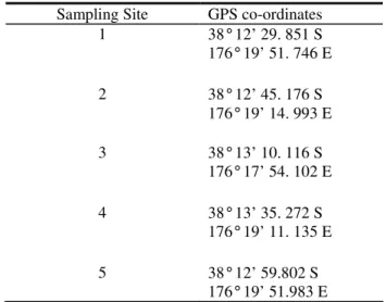
Table 3.0 GPS location of kakahi sampling transects

Sampling Site GPS co-ordinates 1 38° 12’ 29. 851 S 176° 19’ 51. 746 E 2 38° 12’ 45. 176 S 176° 19’ 14. 993 E 3 38° 13’ 10. 116 S 176° 17’ 54. 102 E 4 38° 13’ 35. 272 S 176° 19’ 11. 135 E 5 38° 12’ 59.802 S 176° 19’ 51.983 E

(32)

Kakahi Methods

Once on the boat, mussels were counted and individual length (long axis), width and height (i.e. thickness) of each kakahi shell was measured with callipers before specimens being retuned to the lake.

3.2.2 Kakahi biomass and condition

A sub-sample of 20 kakahi from each depth was kept and taken back to the laboratory and used to calculate biomass and condition indexes following Roper and Hickey (1993). However at 1 and 15 m it was impossible to collect 20 kakahi as numbers were very low at these depths. After each kakahi was shucked, the flesh was oven dried at 60°C for 48 hours and shells air dried for 48 hours. The following two physical condition indices were calculated as in Roper and Hickey (1994) as a measure of physiological stress.

3.2.3 Sediment

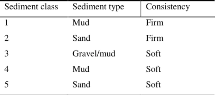
At each site and depth a visual assessment of sediment type and composition was recorded and classified into categories. Table 3.1 describes the basic sediment type as being either mud, sand or gravel and consistency classified as firm or soft.

Table 3.1 Visual assessment table of the sediment at each site

Sediment class Sediment type Consistency 1 Mud Firm 2 Sand Firm 3 Gravel/mud Soft 4 Mud Soft 5 Sand Soft CIflesh:shell weight =

dry flesh weight (mg) shell weight (g)

CIflesh:shell volume =

dry flesh weight (mg) shell volume (ml)

(33)

Kakahi Methods

22 3.2.4 Lake bottom slope

Along each sampling transect starting near-shore the lake bottom gradient or steepness was quantified from a boat using an echo sonar combined with Global Positioning System chart plotter (Garmin GPSMAP 168 Sounding) and associated software to record GPS co-ordinates and associated depth every few seconds. This data was later used within the Ocean Data View programme to plot bathymetric profiles of each transect where kakahi were sampled. Using these profiles, relative estimates of the lake bottom gradient along transects could be made by dividing the depth where kakahi were sampled by distance from shore.

3.2.5 Macrophytes

Macrophyte data was recorded when conducting initial surveys of potential transect sites. In particular percent weed cover of the lake bottom was estimated and dominant species recorded. The results of LakeSPI weed survey data was also consulted specific to Lake Rotokakahi (Clayton, 2002; Clayton, pers.com, 2007)

3.2.6 Depth

Water depth was measured initially using a depth sounder, then secondly by SCUBA depth gauges when diving at each depth.

3.2.7 Dissolved oxygen, chlorophyll a fluorescence and temperature

Dissolved oxygen chlorophyll a fluorescence and temperature measurements were obtained from the CTD profile data. These data was not collected directly from each kakahi transect site but from the CTD site nearest each transect site and averaged over the monitoring period (13 months) at 1 m 5 m, 10 m and 15 m depths.

An oxygen sensor (Greenspan Technology, Model DO300) was deployed in close proximity to site 1 (38° 12’ 30. 819S, 176° 19’ 51. 983E ) (Fig. 3.1) at depths 10 and 15 m from 28 February to 19 March and from 19 March to 1 April respectively to record dissolved oxygen and temperature every 30 minutes. At

(34)

Kakahi Methods

both depths the sensor was positioned 1 m off the bottom (i.e. 9 m and 14 m). This was done in order to closely observe possible fluctuations in dissolved oxygen near the sediment - water interface and to better represent dissolved oxygen levels experienced by kakahi in the immediate vicinity. It was noted that times when dissolved oxygen were recorded were not updated by the sensor and the senor stopped recording unexpectedly towards the end of the data set.

3.2.8 Data analysis

Monthly temperature, oxygen and fluorescence data was averaged annually at 1 m, 5 m, 10 m and 15m to allow comparison with kakahi data. Simple linear regression plots were initially used to observe any relationship between kakahi density and biomass and individual environmental data. If data appeared produced a non-linear pattern, a non linear regressional analysis was used. A Pearsons product momentum correlation matrix was then constructed including all variables measured in this study to examine all variable interactions.

Using the statistics programme STATISTICA (V.8) a multiple regression analysis was performed on kakahi density and biomass against all environmental variables. Kakahi condition and biomass data as dependant variables were compared against depth using a one way Analysis of Variance (ANOVA).

(35)

Water Quality Results

24

Chapter 4 Water Quality Results

4.1 Temporal and spatial variations in temperature, dissolved oxygen

and chlorophyll fluorescence

4.1.1 Temperature

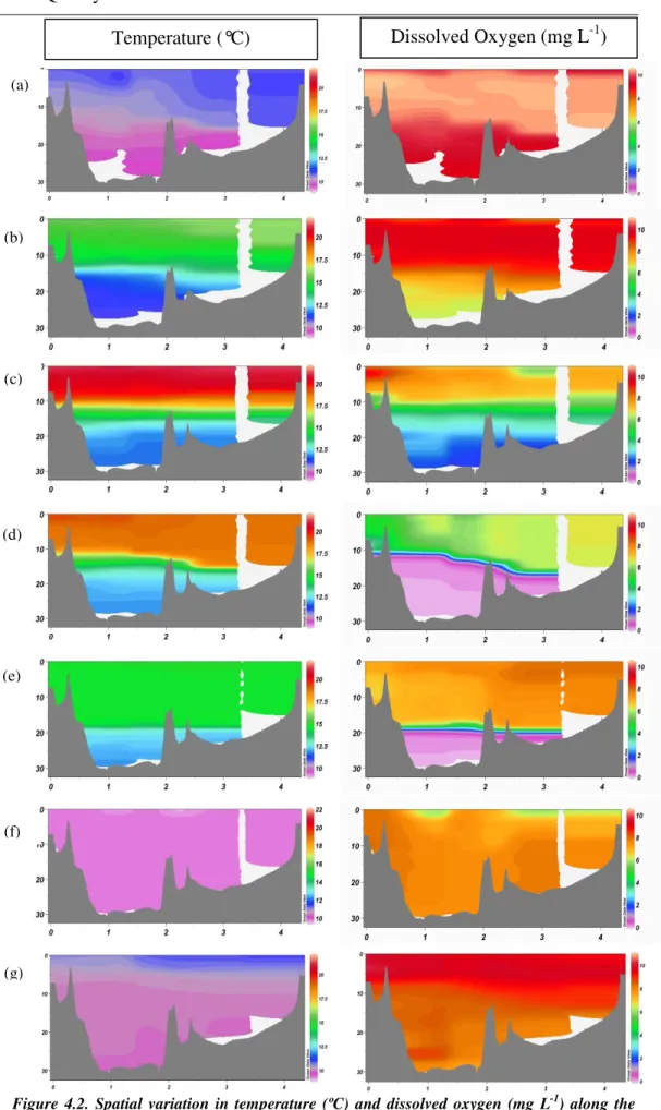
Lake Rotokakahi is monomictic, and stratified for approximately eight months annually, from October 2006 to May 2007. Water temperatures ranged from approximately 21.6 to 9.8 °C in the epilimnion and 9.8 to 11.0 °C in the bottom of the hypolimnion over the annual cycle (Fig. 4.1 a). Turnover occurred at the start of winter, in June, when the water column became isothermal (temperature 12.4

°C). During the winter mixed period (June-September) temperatures remained between 12.4 and 9.6 °C (Fig. 4.1 a). The metalimnion was located between 10 and 18 m depth during the stratified period. During January and February the lake was most strongly stratified, with the metalimnion beginning to deepen in March and continuing to deepen until turnover in June (Fig. 4.2). Evidence of thermocline tilting can be seen in April-March (Fig. 4.2d) shown by an accumulation of warmer water at the north eastern end, which was exposed to prevailing winds from the west of up to 20 knots.

4.1.2 Dissolved oxygen

Dissolved oxygen concentrations changed with a pattern similar to that of seasonal temperature variations through the year (Fig 4.1 b). The hypolimnion was anoxic for four months of the year (February-May), and concentrations during this time were between 0.14 and 0.08 mg L-1 while during winter turnover entire lake water was well oxygenated with concentrations in the range 6.2-9.5 mg L-1. The epilimnion was generally well oxygenated (> 7.1 mg L-1) during stratification but with a pattern of lower values during warmer water temperatures, and with signs of reduced levels of 6.0 and 6.1 mg L-1 in March and June, respectively (Fig. 4.1b).

(36)

4.1.3 Chlorophyll fluorescence

Measurements of chlorophyll fluorescence are given only as relative values but numerical values approximate to concentrations of chlorophyll a in units of µg L

-1_{. Fluorescence measurements recorded ranged from 13 µg L}-1_{(September 2006}

06 to January 2007) to concentrations up to 127 µg L-1 in April, May and August during winter bloom events. Solar quenching of phytoplankton was observed at in the surface waters at depths between 0 and 5 m, most notably in April to May 2006, and August through to September 2007 (Fig. 4.3). These occurrences were notable by progressively lower fluorescence towards the water surface during periods of when there was high solar radiation.

Chlorophyll fluorescence was elevated in the upper 10 m late in the period of thermal stratification, particularly from March to May and during winter mixing from July to August (Fig. 4.3). Fluorescence was generally greatest during late summer and winter and is related to chlorophyll a as 0.5722 • chlorophyll a.

(37)

Water Quality Results 26 S D e p th ( m ) (a) (b) (c) Year fraction

Figure. 4.1 Temperal variation in (a) temperature in °C, (b) dissolved oxygen in mg L-1 and(c) chlorophyll fluorescence over the lake depth for the sampling period of 18/09/06 to 14/09/07. letters indicate month and date when CTD profiles were taken

(38)

Dissolved Oxygen (mg L-1) Temperature (°C)

Figure 4.2. Spatial variation in temperature (ºC) and dissolved oxygen (mg L-1) along the CTD transect. x axis = distance (km), y axis = depth (m). Colour bars indicate temperature and dissolved oxygen gradients. (a) = September 06, (b) = November, (c) = January, (d) = March, (e) = May, (f) = July, (g) = September 07

(a) (b) (c) (d) (e) (f) (g)

(39)

28

Figure 4.3. Spatial variation in fluorescence (µg L-1) along the CTD transect. x axis = distance (km), y axis = depth (m). Colour bars indicate fluorescence gradients. (a) = September 06, (b) = November, (c) = January, (d) = March, (e) = May, (f) = July, (g) = September 07 (a) (b) (d) (c) (e) (g) (f)

(40)

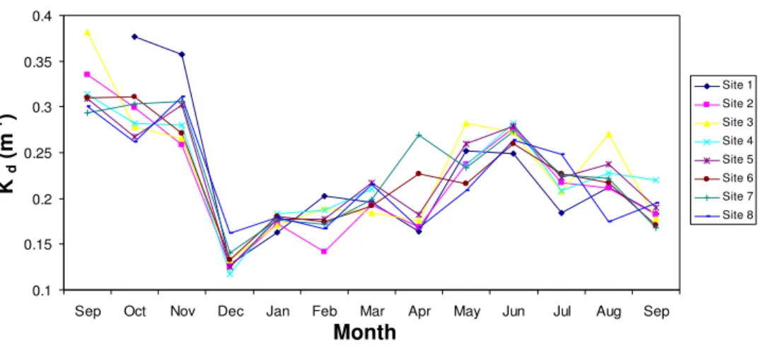
4.2 Light attenuation (kd ), Secchi depth and Euphotic depth

The light attenuation coefficient was fairly consistent between stations on each sample day (Fig. 4.4). From September to November 2006 kd was high (0.26-0.38

m-1) compared with the remaining months of sampling (0.12-0.28 m-1). By December 2006 kd had decreased rapidly and reached a minimum over the year of

sampling. Following December kd gradually increased until June 2007, before

decreasing for the remaining 3 months of sampling.

Secchi disk depths (Fig 4.5) were relatively high, between 4.7 and 6.5 m from September 2006 to January 2007, when chlorophyll a levels were mostly lower. From February to July 2007 Secchi depth then decreased to an average of 3.96 m before increasing again from July 2007 as chlorophyll a concentrations again decreased.

Euphotic depth (Table 4.1) was higher in spring to early summer averaging 15 m from September 2006 to December then was lower for the remaining period (average = 10.7 m) although did increase to 13.8 m in September 2007.

4.3 Chlorophyll a

Chlorophyll a concentrations, measured as solvent-extracted pigment, were generally fairly constant from September 2006 to January 2007, throughout the water column and in the outflow (Fig. 4.5). During the first 6 months of sampling,

K d ( m -1 ) Month 0.1 0.15 0.2 0.25 0.3 0.35 0.4

Sep Oct Nov Dec Jan Feb Mar Apr May Jun Jul Aug Sep

Site 1 Site 2 Site 3 Site 4 Site 5 Site 6 Site 7 Site 8

(41)

30 chlorophyll a ranged from 0.62 to 1.02 µg L-1. From Februrary 2007 chlorophyll a increased and became more variable at all locations, excluding the 27 m depth. At this depth chlorophyll a gradually increased from November 2006 to August 2007 and then decreased dramatically by September 2007. Two exceptional increases in chlorophyll a occurred within the outflow (76 µg L-1 ) and at 15 m depth (92 µg L

-1 _{) in April and May, respectively (Fig. 4.5). These high values correspond to}

elevated chlorophyll a fluorescence values observed above the thermocline in these months (Fig. 4.3 d and e).

Sep Oct Nov Dec Jan Feb Mar Apr May Jun Jul Aug Sep Zeu (m) 16.2 13.4 15.25 15.0 11.8 9.8 10 10.8 9.6 9.5 9.8 11.1 13.8 Kd (m-1 ) 0.3 0.3 0.3 0.1 0.2 0.2 0.2 0.2 0.3 0.3 0.2 0.2 0.2 Secchi (m) 6.5 5.4 6.1 6.0 4.7 3.9 4.0 4.3 3.9 3.8 3.9 4.5 5.5 0 10 20 30 40 50 60 70 80 90 100

Month C h lo ro p h y ll a ( µ g /L -1 ) 0 0.5 1 1.5 2 2.5 3 3.5 4 4.5 5 5.5 6 6.5 7 S e c c h i d e p th ( m )

0 m I.S 15 m 27 m Outflow Secchi

Fig. 4.5 Chlorophyll a and Secchi disk depth measurements taken at 0 m, Integrated (0 - 10 m), 15 m, 27 m and at the outflow

Table 4.1 Comparison of euphotic depth Zeu, light extinction coeffieicent Kd and Secchi disk

(42)

4.4 Phytoplankton and zooplankton abundance

4.4.1 Phytoplankton

The dominant phytoplankton over the entire period of sampling were from the dinoflagellate, diatom, chlorophyte and cyanobacteria phyla. At 0 m chlorophyte species were most abundant from September 2006 to May 2007 (12-75%) followed by diatoms and dinoflagellates (Fig. 4.6 a). Cyanobacteria species were present in the first half of the year reaching 60% abundance in November then reducing to less than 10% in December onwards. From May to September both diatoms and dinoflagellates dominant with diatoms progressively increasing to 90% abundance in September. Chrysophytes and euglenophytes were present in low densities at the beginning and end of the monitoring period.

At 15 m from September 2006 to February 2007 diatoms and cyanobacteria remained dominant, with diatoms reaching 96% abundance in November 2006 (Fig. 4.6 b). From March onwards dinoflagellates were most dominant, with abundances of 46-79%. Chlorophytes were present in lower denisities, between 0.3-25 % abundance.

Dominant species included the chlorophyte Staurastrum spp., the diatoms Fragilaria crotonensis., Aulacoseira granulata. and Asterionella formosa, the dinoflagellate Ceratium hirundella the cyanobacteria Anabaena flos aquae and Anabaena spiroides and the Chrysophyte Dinobryon cylindricum at both 0 and 15 m.

Quantitative cell counts were not determined at 0 m as samples as samples were obtained by drag net and therefore were concentrated. Generally cell counts taken at 15 m (Fig. 4.7) range from 844 to < 10 cell ml-1. Diatom and dinoflagellates reached peaks of 2,821 cell ml-1 and 1,891 cell ml-1 in February and March, respectively, while cyanobacteria were highest in December peaking at 514 cell-1 .

(43)

Water Quality Results 32 C e ll s m l -1 0 500 1000 1500 2000 2500 3000

Sept Oct Nov Dec Jan Feb Mar Apr May Jun Jul Aug Sept

Cyanobacteria Dinoflagellates Diatoms Chrysophyta Chlorophyta

Figure. 4.7 Cell counts of phytoplankton phyla taken at 15 m depth

Month R e la ti v e c o m p o s it io n ( % )

Figure. 4.6 Relative composition of phytoplankton phyla at 0 m (a) and 15 m (b)

R e la ti v e c o m p o s it io n (% ) 0 20 40 60 80 100

Cyanobacteria Dinoflagellates Diatoms Chrysophyta Chlorophyta

Month 0 20 40 60 80 100

Month a

(44)

Water Quality Results 4.4.2 Zooplankton

Most zooplankton groups showed large monthly fluctuations in relative abundance, ranging from >90% to >5% (Fig. 4.8 a). Rotifer abundances appeared to be negatively related cladocerans and copepods abundances while nauplii remained at low abundances with little monthly variation. From March to September 2007 cladoceran, copepod and rotifer abundances gradually increased. Nauplii roughly followed copepod abundances.

Dominant zooplankton species represented in each group included Bosmina meridionalis (Cladocera), Calamoecia lucasi (Calanoid copepods), Keratella sp. Filinia sp., Trichocerca similes and Asplanchna sp. (Rotifera) and calanoid nauplii.

Densities recorded from 0 to 10 m were very high for rotifers in January and March (>300 L-1), however, underwent large fluctuations between (February and April 2007) when there were very low densities (Fig. 4.8 b). Cladocerans and copepod densities both peaked in February and then had low densities thereafter. Over the entire period of sampling, average annual densiity recorded was 32 zooplankton L-1. Zooplankton relative composition and cell counts were not determined in October.

(45)

34

4.5 Nutrients

Concentrations of phosphate were low (0.001-0.010 mg L-1) at most sampling locations during the monitoring period. However samples from 27 m depth and the inflow in particular showed marked increases during February to June 2007 and from April to August 2007, respectively (Fig. 4.9).

Concentrations of total phosphorus (TP) were mostly higher in the inflow (0.05-0.092 mg L-1) compared with other lake site concentrations (0.005-0.066 mg L-1) including the outflow, for which concentrations were mostly lower (Fig 4.9).

Ammonium concentrations at 27 m were higher than most depths including the lake inflow and outflow. Concentrations at 27 m depth peaked in May (0.073 mg L-1) before decreasing to a minimum in July and remaining low thereafter (Fig

Figure. 4.8 Relative composition (%) (a) and composition (ml-1) (b) of zooplankton phyla within the integrated sample (1-10 m)

0 100 200 300 400 500

Cladocerans Copepods Rotifers Naupilii

Month Month 0 20 40 60 80 100

Z o o p la n k to n m l -1 R e la ti v e c o m p o s it io n ( % ) a b

(46)

4.9). Ammonium at all other sites showed similar trends, ranging from 0.001-0.024 mg L-1. In December, concentrations of ammonium at 0 m, the integrated sample (0-10 m depth), 27 m and the outflow were greater (0.016-0.019 mg L-1) than at any other time during sampling for the respective sampling sites.

From January 2007 nitrate generally decreased except for an increase in August. Similar to other nutrients, nitrate concentrations in the inflow were generally higher than all other sampling sites on the same day of sampling. At 27 m depth nitrate concentrations were greatly reduced relative to ammonium.

Concentrations of total nitrogen gradually increased from September 2006 to March 2007, then tended to plateau at all sites until completion of sampling. One notable feature was a relatively large peak in TN (0.587 mg L-1) in the outflow in August.

(47)

Water Quality Results 36 0 0.02 0.04 0.06 0.08 0.1

0 0.02 0.04 0.06 0.08 0.1

0 0.005 0.01 0.015 0.02 0.025

0 0.02 0.04 0.06 0.08

0 0.2 0.4 0.6 0.8

0 m I.S 15 m 27 m Outflow Inflow

P O4 (m g L -1 ) T P (m g L -1 ) N O3 (m g L -1 ) N H4 (m g L -1 ) T N ( m g L -1 )

Figure. 4.9 Total and dissolved nutrients from 0 m, integrated (0 - 10 m), 15 m, 27 m, outflow and the inflow

(48)

4.6 Modelling using DYRESM-CAEDYM

4.6.1 Temperature

Fig. 4.91 presents a comparison of temperature data simulated with the model DYRESM against measured data from CTD profiles. Temperature was predicted by the model most accurately at the water surface (Table). At a depth of 14 m the temperature simulated with the model were too high during stratification (January-April). In the hypolimnion (26 m) modelled temperature data was generally slightly lower than the field data, however simulations captured the slight increase in temperature from June-July.

Figure. 4.91 Temperature observed and modelled data at 0 m (a), 14 m (b) and 26 m (c).

5 10 15 20 25 08/31/06 10/20/06 12/09/06 01/28/07 03/19/07 05/08/07 06/27/07 08/16/07 Date T e m p e ra tu re ( °C ) Model Field 5 10 15 20 25 08/31/06 10/20/06 12/09/06 01/28/07 03/19/07 05/08/07 06/27/07 08/16/07 Date T e m p e ra tu re ( °C ) Model Field 5 10 15 20 25 08/31/06 10/20/06 12/09/06 01/28/07 03/19/07 05/08/07 06/27/07 08/16/07 Date T e m p e ra tu re ( °C ) Model Field (a) (b) (c)

(49)

38 4.6.2 Dissolved Oxygen

The model simulations captured the general pattern of variations in dissolved oxygen, which were associated generally with changes in stratification (Fig. 4.92). At the surface the model did not represent well the peaks and troughs in the observed dissolved oxygen concentrations. Simulations of dissolved oxygen tended to be too high throughout the water column during the period of lake mixing. At 14 m depth the model did show the large reduction in dissolved oxygen that occurred from December 2006 to March 2007, however, during the entire monitoring period simulated concentrations were generally too high. At 26 m the low dissolved oxygen concentrations during the period of summer stratification were mostly well predicted, at least until the period of winter mixing (Fig.4 .92 c).

(50)

Water Quality Results 0 2 4 6 8 10 12 8/31/06 10/20/06 12/9/06 1/28/07 3/19/07 5/8/07 6/27/07 8/16/07 Date O x y g e n ( m g /L ) Model Field 0 2 4 6 8 10 12 8/31/06 10/20/06 12/9/06 1/28/07 3/19/07 5/8/07 6/27/07 8/16/07 Date O x y g e n ( m g /L ) Model Field 0 2 4 6 8 10 12 8/31/06 10/20/06 12/9/06 1/28/07 3/19/07 5/8/07 6/27/07 8/16/07 Date O x y g e n ( m g /L ) Field Model

Figure. 4.92 Dissolved oxygen observed and modeled data at 0 m (a), 14 m (b), 26 m (c).

(a)

(b)