Master Thesis
Upcompiling Legacy Code to Java
Author Urs F¨assler
Supervisor ETH Z ¨urich UC Irvine
Prof. Dr. Thomas Gross Prof. Dr. Michael Franz Dr. Stefan Brunthaler Dr. Per Larsen
Urs F¨assler: Upcompiling Legacy Code to Java,© September7,2012
This work is made available under the terms of the Creative Com-mons Attribution-ShareAlike 3.0 license, http://creativecommons. org/licenses/by-sa/3.0/.
A B S T R A C T
This thesis investigates the process of “upcompilation”, the transfor-mation of a binary program back into source code. Unlike a decom-piler, the resulting code is in a language with higher abstraction than the original source code was originally written in. Thus, it supports the migration of legacy applications with missing source code to a virtual machine. The result of the thesis is a deeper understanding of the problems occurring in upcompilers.
To identify the problems, we wrote an upcompiler which transforms simple x86 binary programs to Java source code. We recover local
variables, function arguments and return values from registers and memory. The expression reduction phase reduces the amount of vari-ables. We detect calls to library functions and translate memory al-location and basic input/output operations to Java constructs. The structuring phase transforms the control flow graph to an abstract syntax tree. We type the variables to integers and pointers to integer. In order to optimize the produced code for readability, we developed a data flow aware coalescing algorithm.
The discovered obstacles include type recovery, structuring, handling of obfuscated code, pointer representation in Java, and optimization for readability, to only name a few. For most of them we refer to related literature.
We show that upcompilation is possible and where the problems are. More investigation and implementation effort is needed to tackle spe-cific problems and to make upcompilation applicable for real world programs.
A C K N O W L E D G E M E N T S
I like to thank Professor Michael Franz for the invitation to his group and making this work possible. A special thank goes to Stefan Brun-thaler and Per Larsen for the discussions and suggestions. I thank Professor Thomas Gross for enabling the work. Finally, I like to thank the supporters of free software for providing all tools needed for this work.
C O N T E N T S 1 i n t r o d u c t i o n 1 1.1 Problems . . . 1 1.2 Scope . . . 3 2 r e l at e d w o r k 4 3 i m p l e m e n tat i o n 5 3.1 Low level phases . . . 5
3.1.1 Disassembler . . . 6
3.1.2 Variable linking . . . 7
3.1.3 Function linking . . . 7
3.1.4 Condition code reconstruction . . . 8
3.1.5 Stack variable recovery . . . 9
3.1.6 Expression reduction . . . 11
3.1.7 Function replacement . . . 12
3.1.8 Replacing arrays with variables . . . 13
3.1.9 SSA destruction . . . 13
3.2 High level phases . . . 14
3.2.1 Structuring . . . 15
3.2.2 Linking . . . 15
3.2.3 Statement normalization . . . 17
3.2.4 Reconstructing types . . . 17
3.2.5 Pointer access encapsulation . . . 18
3.2.6 Coalescing . . . 19
3.2.7 Expression normalization . . . 20
3.2.8 Generating Java code . . . 20
4 e va l uat i o n 22 4.1 Discussion . . . 22
4.1.1 Function pointers . . . 22
4.1.2 Function argument reconstruction . . . 23
4.1.3 Non returning functions . . . 23
4.1.4 Jump tables . . . 24 4.1.5 Structuring . . . 25 4.1.6 Stack variables . . . 25 4.1.7 Library calls . . . 26 4.1.8 Tail calls . . . 26 4.1.9 Aliasing of registers . . . 26
4.1.10 SSA as intermediate representation . . . 27
4.1.11 Coalescing unrelated variables . . . 27
4.1.13 Obfuscation and optimization . . . 29
4.1.14 Functional programming languages . . . 30
4.2 Performance . . . 32 4.2.1 Upcompiler . . . 32 4.2.2 Programs . . . 33 5 c o n c l u s i o n a n d f u t u r e w o r k 35 5.1 Conclusion . . . 35 5.2 Future Work . . . 36 5.2.1 Type recovery . . . 36 5.2.2 Generality . . . 36
5.2.3 Optimization and code metrics . . . 37
a b i b l i o g r a p h y 39 b l i s t i n g s 42 c l i s t o f f i g u r e s 43 d a p p e n d i x 44 d.1 Glue code . . . 44 d.2 Testcases . . . 45 d.2.1 fibloop . . . 45 d.2.2 fibrec . . . 51 d.2.3 fibdyn . . . 53 d.2.4 bubblesort . . . 56
1
I N T R O D U C T I O N
Legacy applications without source code become a considerable prob-lem when their target processors are no longer available. Cross-compilation or binary translation, i.e., translating the binary appli-cation to another instruction set architecture (ISA), are not sustain-able solutions, as the target architecture also becomes obsolete even-tually.
In contrast, the Java virtual machine (JVM) decouples the source code from any particular processor. The JVM itself runs on a wide range of processors. As the specification of the JVM as also the Java language are publicly available and there exist free and open source implemen-tations of the JVM and Java compiler, it provides a future proof archi-tecture. Moreover, the language is widely used in the industry and academic communities. If we are able to translate binaries into Java source code, they do not only compile for the JVM but also allows programmers to fix, improve or extend the applications.
In this thesis we investigate the process of “upcompilation”. An up-compiler translates a binary program into source code of a language of higher abstraction than the program was originally written in. In comparison to decompilation, upcompiler face the additional chal-lenges of bridging a broader semantic gap. The gain of this thesis is a deeper understanding of the problems occurring when building a real world upcompiler.
1.1 p r o b l e m s
Disassembly and decompilation are already difficult problems since a compiler destroys a lot of information. As we want to upcompile, we do not only have the same problems but also new ones. The reason is that we want to go to an higher abstraction than the code was before compiling. Figure1.1 on the following page shows the levels
high low abstraction C Machine Code Assembly C Java compiler disassembler decompiler upcompiler
Figure1.1: Machine code abstraction level. The reconstructed C code
on the right side is on a lower abstraction than the original because information was destroyed during compilation.
On the disassembly level, we have to distinguish between code and data. In the general case, it is considered as a hard problem [18].
Since we have the entry point to the binary and follow all paths, we avoid this problem. Disassembly the binary gets difficult if code ob-fuscation is used or the code is self modifying.
Decompilation is more difficult as we want to recover variables, their types, and high level language constructs. A value can be stored in a register, memory or both. But not every value in a register or memory represents a variable. As the machine needs to store the result of ev-ery operation, several registers are used. It is not clear which values belonged to a variable and which ones are for temporary storage. In the absence of debugging information, only a small amount of infor-mation about types is available. This includes the size of an integer or if it is a signed value. Moreover, there is no explicit information about composite types like arrays or records.
Optimization frequently moves code around, which makes the recov-ery of high level language constructs difficult or impossible. Never-theless, since C has a low machine code abstraction, several problems are not so hard if we do not care about readability of the resulting code. Otherwise, optimizations like function inlining and loop un-rolling have to be detected and reverted. Furthermore, the compiler or linker add helper code to the program. Such code has to be de-tected and removed, too.
Upcompilers have the additional challenge of bridging the seman-tic gap. This is the problem that a language of higher abstraction has more constraints than the language of the original program. For example, C or Object Pascal allows to access every memory address with a pointer of any type. In Java or Ruby, neither accessing memory nor arbitrary type casts are possible.
1.2 s c o p e
As we have limited resources, we restricted the possible set of input programs. This allows us to implement all parts of the upcompiler. We only worked with 32-bit x86 binaries compiled by Clang, a C
compiler with LLVM as back end. All binaries need to be in the Ex-ecutable and Linkable Format (ELF). We only support dynamically linked libraries, and only a small number of library calls. Those are
printfandscanfwith simple static format strings as well asmalloc
andfree. Multi-threading, signals and function pointers are not sup-ported. Parameters to functions have to be passed on the stack. Sup-ported data types are signed integers and pointers to integers.
Obfuscated code, hand written assembly code, computed jumps, just-in-time compilers, self modifying code and similar techniques are not considered in our implementation.
2
R E L AT E D W O R K
First decompilers are mentioned in the1960’s by Halstead [19]. Back
then, they had the same motivation as we have for the upcompiler: It was used to guide the migration of programs to a new computer generation.
Modern decompilation is based on the work of Cifuentes [11]. Since
then, findings in research and industry changed and improved com-pilers. Most notably, the static single assignment form (SSA) [15] is
used by many modern compilers. Its usefulness for decompilation is described by Mycroft [25] and Emmerik [18].
Upcompiling binaries to Java or similar targets is a new research topic. Nevertheless, it should be possible to reach the same goal with the usage of several existing tools. As there exists a lot of research on decompilers, it seems obvious to first decompile a binary and then use a C to Java converter. There exist decompilers like Boomerang [1]
or REC [2] producing C like code, and C to Java converter like C2J
[3], but they all seem to be immature or incomplete.
It should be possible to use tools, such as RevGen/s2e [10] to
de-compile binaries to LLVM IR. From there, LLJVM [26] produces Java
bytecode. Many Java decompilers exist; some of them may be able to work as the last step to retrieve Java source code. Unfortunately, both RevGen and LLJVM are still prototypes.
NestedVM [7] is able to translate MIPS binaries to Java Bytecode.
The authors choose MIPS because of “the many similarities between the MIPS ISA and the Java Virtual Machine” (Alliet and Megacz [7,
page3]). Since our motivation is to upcompile legacy applications for
3
I M P L E M E N TAT I O N
The upcompiler is written in Java using additional libraries. ELF parsing is based on the source code of Frida IRE [20]. DiStorm3[16]
disassembles the binary. JGraphT [4] provides the graph
infrastruc-ture.
The translation from machine code to Java is split up into several phases. Every phase can perform multiple passes over the internal representation. We use a control flow graph (CFG) for the low level representation and later an abstract syntax tree (AST) for the high level representation.
We describe the phases of the upcompiler in the following sections. For practical reasons, they are not strictly in the same order as they are implemented. In most sections, a listing or figure illustrates code snippets before and after the phase. At the end of every section, we indicate the relevant classes of the upcompiler with an arrow (⇒).
3.1 l o w l e v e l p h a s e s
The whole program consists of a set of functions. Every function is represented as a CFG where the vertices are basic blocks. There is exactly one vertex with an in-degree of zero, the entry point of the function. A function has one or more exit points. The registers and recovered variables are in SSA form.
Every basic block is constructed in the same way. It is identified by the memory address of its first instruction, even if this instruction is deleted during the process. At the beginning, zero or more phi functions are allowed. They have a key/value pair for every incoming edge of the basic block. The key is the ID of the source basic block of the edge and the value is the expression which is used when the control flow transfers from the mentioned basic block. Then, zero or more statements follow. At the end, there is exactly one jump or
The syntax is intuitive, only the jump statement needs a description. It takes two arguments, an expression and a list of basic block iden-tifiers. The expression is evaluated and that value is used as index for the list. Finally, the control flow transfers to the basic block at the mentioned index. This representation models all occurring jumps. Listing3.1on the current page shows the use cases.
1 jump( 0, [BB_N] )
2 jump( a < 10, [BB_F, BB_T] ) 3 jump( a, [BB_0, BB_1, BB_2] )
Listing3.1: The 3 different use cases of the jump statement. Line 1
contains an unconditional jump, line2 represents a jump
depending on a boolean condition and line3 contains a
multi-branch.
3.1.1 Disassembler
First, the upcompiler disassembles and splits the binary program into basic blocks. The disassembly library provides the decoded assembly instructions which are directly translated into our intermediate rep-resentation.
In addition, we load the dynamic library section for the later resolu-tion of addresses to library funcresolu-tion names as discussed in Secresolu-tion
4.1.7on page26.
We detect all functions of the call graph with the entry point of the binary as the root vertex. Whenever a call instruction occurs during parsing, we add the destination address to a work queue. Already parsed functions and library functions are excluded.
Basic blocks of a function are parsed similarly. The first basic block starts at the address of the function. For a conditional jump, we put the address of the following instruction and the jump destination to a work queue. If the jump is unconditional, only the destination address is added. Those jump instructions also terminate the basic blocks. In addition, function return or program abort instructions also terminate a basic block. If a jump instruction points into an already parsed basic block, we split that basic block at the destination address. Before parsing an instruction, we check if there is already a basic block starting with this instruction. If so, we add a jump to that basic block. We discuss the handling of jump tables in Section4.1.4
Listing 3.2 on this page is an example of a basic block after this phase.
⇒
phases.cfg.Disassembler 1 0x8048480: 2 EDX:22 := ’ESI’ 3 ESI:23 := ’ECX’4 ESI:24, C:24, P:24, A:24, Z:24, S:24, O:24 := (’ESI’ + ’EDX’) 5 EDI:25, P:25, A:25, Z:25, S:25, O:25 := (’EDI’ - 0x1)
6 ECX:26 := ’EDX’
7 jump( (’Z’ == 0x0), [0x804848b, 0x8048480] )
Listing3.2: A basic block after the disassembly phase.
3.1.2 Variable linking
In this phase we link all variables by converting them to SSA. To get the positions for the phi functions, we implemented a generic domi-nator tree algorithm as described by Cooper et al. [14] and a generic
dominance frontier algorithm as in Cooper and Torczon [13].
We only consider registers and flags as variables as we have no alias-ing information about memory. Registers can also be aliased, for example EAXwithAL, but we know all possible cases and treat them accordingly (see Section4.1.9on page26for a discussion about
alias-ing).
⇒
phases.cfg.VariableLinker3.1.3 Function linking
After this phase all function calls are linked to the function definition. We also detect the variables used to return values from the function. Library functions are assumed to have C calling convention (cdecl), therefore we know which variable holds the return value. However, it is not known for private functions, as the compiler can use any calling convention.
We implemented an algorithm to detect the variables used for return values. With the algorithm shown in Listing 3.3 on the following
is used after a call of f and killed by f, we know that vis a return value off. 1 function dfs( f ) 2 kill[f] := gen[f] 3 visited := visited ∪ f 4 for g ∈ callee[f] 5 if g ∈/ visited 6 dfs( g )
7 kill[f] := kill[f] ∪ kill[g]
8 kill[f] := kill[f] - save[f]
Listing3.3: Algorithm to detect killed variables. Called on a function f, we get the killed variables in kill[f]. The variables written by a function fare in gen[f], the ones saved on the stack are insave[f].
After we added the variables with the return values, we run the vari-able linker again. A subsequent step removes all superfluous phi nodes. This ensures that all variable references are linked to a defini-tion.
⇒
knowledge.KnowKilledByFunction phases.cfg.FunctionVariableLinker3.1.4 Condition code reconstruction
In this phase we replace the flag tests in conditions with relational operators. Depending on the flags tested and the instruction generat-ing the flags, we know the relation. After this step, all flags should be removable. Listings3.4on the current page shows an example.
⇒
phases.cfg.ConditionReplacer1 C:27, P:27, A:27, Z:27, S:27, O:27 := (ECX:23 and ECX:23) 2 jump( (Z:27 == 0x0), [0x804850f, 0x8048500] )
1
2 jump( (ECX:23 != 0x0), [0x804850f, 0x8048500] )
Listing3.4: Before and after the condition replacement phase. The andoperation is removed since it is no longer used.
3.1.5 Stack variable recovery
After this phase we have array accesses instead of memory accesses relative toEBPandESP. In addition, the caller and the callee use func-tion parameter instead of memory accesses.
Local variables from the original source program are translated to registers or memory accesses relative to the stack pointers. If a mem-ory access is above of EBP, we know that this is an argument. By checking all memory accesses we find the highest offset relative to
EBPand therefore the number of arguments. This works because we only have integers and pointers as arguments. BelowEBPwe find the saved registers and after them the local variables and the arguments for the callees. There is no need to separate these. Figure 3.1 on the
following page shows the phases of variable recovery.
In the callees, we replace memory accesses to the argument area by accesses to the newly introduced argument-variables. At every call expression, we insert the actual arguments. The arguments are the stack-array elements at the corresponding positions; the number of arguments is known from the callee.
The area for local variables is seen as an array. Memory accesses are translated into array accesses. If there is an access with a static array offset, we split the array at that position. This separates the different variables of each other. For the limitations, see Section4.1.6
on page25.
Listing 3.5 on this page shows the difference before and after this
phase.
⇒
phases.cfg.FunctionRecovery 1 *(ESP:0 + 0x0) := 0x80486d0 2 call ’puts’() 1 loc0[0x0] := 0x80486d0 2 call ’puts’(loc0[0x0])Listing3.5: Changes of the stack variable recovery phase. Memory
accesses relative to the stack pointer are replaced by intro-ducing local arrays. Function calls get their actual argu-ments.
(a)
(b)
(c)
esp esp+4 ebp-52 ebp-48 ebp-8 ebp+4 ebp+8
loc0[1] loc1[4] loc5[1] loc6[10] arg0 arg1
lar0 lar1 lar5 loc6[10] arg0 arg1
0 1 ... 5 6 ... 16
Figure3.1: Transformation of stack memory to local variables and
ar-guments. The arrows on top illustrate direct pointer ac-cesses, the numbers at the bottom the array indices. Saved registers, stack pointer and the return address are in the area betweenebp-8 andebp+4. They are not used in the recovering process.
First, there are only memory accesses relative to espand
ebp as on row (a). We consider this part of the stack to be an array. The stack variable recovery phase (see page
9) splits the array at the indices of memory accesses,
re-sulting in row (b). We also replace the stack area above
ebp+4 with function argument variables. After the phase where we replace arrays with variables (see page 13) we
get row (c). The variables loc0, loc1 andloc5 are intro-duces since there was no index calculation on the corre-sponding arrays.
The variables relative to esp are arguments to functions, the ones relative to ebp are local variables. We see that this function has at least one local integer variable, and one array with 10 elements. Moreover, it calls functions
3.1.6 Expression reduction
This phase reduces expressions by inlining. First, we reduce tau-tological expressions like an addition with zero or dereferencing of address-of operations. Second, we inline expressions. For every us-age of a variable we calculate the cost for inlining the definition of the variable. The cost function counts the number of operation and function calls for an expression. References to variables or memory have no cost. Then we multiply the cost with #usages−1 of this ex-pression. This ensures a cost of zero if the expression is used only once. If the cost is zero, we replace the reference to the expression with the expression itself. Movement of instructions is only allowed within one basic block. Code in phi functions belongs to the previous basic blocks.
A memory model check can prevent the movement of expressions, too. We need the memory model because we do not have information about aliasing for all memory accesses. Moving arbitrary reads with respect to other reads is allowed, arbitrary writes cannot be reordered with respect to other writes or reads. If we know that the memory locations are different, we allow the movement.
Finally, we clean up by removing all definition of unused variables and all statements without effect. These are statements which do not define a variable, do not write to memory and with no function calls. Listing3.6on the current page gives an impression of this phase.
⇒
phases.cfg.MathReduction phases.cfg.SsaReduce1 EAX:17, EDX:17, ST0:17 := call ’malloc’(loc0[0x0])
2 ESI:18 := EAX:17
3 ...
4 EAX:30 := loc3[0x0]
5 ECX:31 := *((EAX:30 * 0x4) + (ESI:18 + -0x4))
6 loc2[0x0] := ECX:31
1 EAX:17 := call ’malloc’(loc0[0x0]) 2
3 ...
4 EAX:30 := loc3[0x0]
5
6 loc2[0x0] := *((loc3[0x0] * 0x4) + (EAX:17 + -0x4))
Listing3.6: Effects of expression reduction. On Line1 it can be seen
how the unused variables are removed, line6 shows the
3.1.7 Function replacement
This phase replaces all calls to known library functions by calls to internal functions. For some functions, likemallocandfree, this is just a replacement of the call destination.
However, functions like scanf and printf need special handling. They have a variable number of arguments, which we do not support in general. We implemented a parser for static scanf and printf
format strings. The current solution requires that the format string resides in the read-only data section of the program.
For every read of an integer, a call to the functionreadIntis inserted and the return value is assigned to the corresponding variable. For every format string of a printf call, we create a new function with the same functionality. Listing3.7on this page shows some examples
of the translation.
⇒
phases.cfg.IoFunctionReplacer phases.cfg.MemoryFuncReplacer 1 loc1[0] := @(loc3[0]) 2 loc0[0] := 0x80486aa 3 call ’scanf’(loc0[0])4 EAX:7 := call ’malloc’(4*loc3[0])
5 ... 6 loc1[0] := EAX:12 7 loc0[0] := 0x80485d5 8 call ’printf’(loc0[0]) 21 0x80485d5: 22 "result: %i\n" 23 0x80486aa: 24 "%i" 1 loc1[0] := @(loc3[0]) 2 loc0[0] := 0x80486aa 3 loc3[0] := call readInt()
4 EAX:7 := call ptrMalloc(4*loc3[0])
5 ... 6 loc1[0] := EAX:12 7 loc0[0] := 0x80485d5 8 call f80485d5(loc1[0]) 9 ... 10 f80485d5: 11 call writeStr("result: ") 12 call writeInt(arg0:0) 13 call writeNl() 14 return
Listing3.7: Replacement of functions. On line1to3one can see how scanf is replaced with information of the format string on line 24. The mallocfunction on line 4 is replaced by ptrMalloc. The call of printf on line 8 is replaced by
a call to a new function with the same semantics as the format string seen on line22.
3.1.8 Replacing arrays with variables
We replace arrays with variables in order to reduce more expressions. Some arrays have only one element, others have no index calculation when accessing them. After an expression analysis does not find an address-of operation on the array, we replace it with a variable. Since variables can not alias each other, another run of the variable reduction phase as in Section 3.1.6 on page 11 simplifies the code
again. Listing3.8 on this page shows the replacement of the arrays
and the result of the reduction, Figure 3.1 on page 10 explains the
idea.
⇒
phases.cfg.ArrayReplacer1 EAX:30 := loc3[0x0]
2 loc2[0x0] := *((loc3[0x0] * 0x4) + (EAX:17 + -0x4))
3 loc1[0x0] := EAX:30
4 call f80486ad(loc1[0x0], loc2[0x0])
5 loc0[0x0] := EAX:17
6 call ptrFree(loc0[0x0])
1 EAX:30 := lar_loc3_0:0
2 lar_loc2_0:0 := *((lar_loc3_0:0 * 0x4) + (EAX:17 + -0x4))
3 lar_loc1_0:0 := EAX:30
4 call f80486ad(lar_loc1_0:0, lar_loc2_0:0)
5 lar_loc0_0:0 := EAX:17
6 call ptrFree(lar_loc0_0:0)
4 call f80486ad(lar_loc3_0:0, *((lar_loc3_0:0 * 0x4) + (EAX:17 + -0x4))) 5
6 call ptrFree(EAX:17)
Listing3.8: Effects of array replacement together with reduction. We
can replace most arrays with variables. Therefore, a re-peated reducing phase can inline and remove a significant amount of copy operations and temporary variables.
3.1.9 SSA destruction
In this phase, we go out of SSA by removing all phi functions. It is necessary since SSA is not compatible with our AST. As a prerequisite, we check that all variables are linked to their definition. Then we rename all variables to be sure that no two variables with the same name exist. This is necessary because we do not support different versions of the same variable name later on.
We use the straight forward SSA destruction algorithm “Method I” described by Sreedhar et al. [30]. It is a simple method with the
downside that it introduces a lot of new variables. The coalescing phase in Section3.2.6on page19 removes many of them. Listing3.9
on the current page gives an idea how the algorithm works.
⇒
phases.cfg.SsaBacktranslator 1 A: 2 jump( 0, [C] ) 3 4 5 6 B: 7 jump( 0, [C] ) 8 9 10 11 C: 12 tmp2 := phi( A::0; B::*(tmp5-4); ) 13 tmp5 := phi( A::tmp1+8; B::tmp5+4; ) 1 A: 2 tmp2_t := 0 3 tmp5_t := tmp1+8 4 jump( 0, [C] ) 5 6 B: 7 tmp2_t := *(tmp5-4) 8 tmp5_t := tmp5+4 9 jump( 0, [C] ) 10 11 C: 12 tmp2 := tmp2_t 13 tmp5 := tmp5_tListing3.9: Before and after SSA destruction. The destruction
algo-rithm adds an additional variable for every phi function. Many of them are removed in the coalescing phase (see section3.2.6on page19).
3.2 h i g h l e v e l p h a s e s
The AST for the second part consists of high-level language con-structs, such as while and if statements. The expressions start by more C like forms with pointer dereferencing. They are successively reshaped into a Java syntax. Finally, we optimize the code and gener-ate the Java files.
We have the following types of statements: • nop • block • call • return • variable definition • assignment • while • do-while • if • switch-case
They are C and Java compatible, but we added more constraints. Loops have no break or continue and the switch-case construct can not have fall-through cases.
During the phases more and more code is dependent on three helper classes. Main in Listing D.1is used to handle the return value of the
main function and the arguments. IoSupportin Listing D.2provides
methods to read from and write to the console. Pointer in Listing D.3 is needed for pointers since they do not have a corresponding
language concept in Java.
3.2.1 Structuring
This is the phase where we transform the CFG into the AST. For ev-ery function, our algorithm searches for specific patterns of vertices in the CFG. If one is found, the algorithm replaces the vertices by a se-mantically equivalent vertex. This is done until only one vertex is left. Figure3.2on the following page shows the structuring process.
It is possible that we can not find a pattern. Such a CFG result from manual jumps in the source program, unknown program constructs and compiler optimizations. We implemented a fallback mode for such cases. In this mode, we simulate the jumps with a switch-case in an infinite loop. It is similar to an interpreter using a switch-based dispatch loop. Every case entry consists of one basic block where we replace the jump at the end of every basic block with a write to the control variable of the switch.
There is room for improvement as we discuss in Section 4.1.5 on
page25.
⇒
phases.ast.Structurer3.2.2 Linking
Here, we insert the definitions for the variables, link the references to them, and link function references to their definition, too. Con-trary to the SSA representation, we need a specific definition for ev-ery variable. To make it simple we insert all variable definitions in the beginning of the function.
In addition we link and rename the functions. As we focus on stripped binaries, we rename all functions, even if the name of the function is available. The entry-function gets the name “main”, all others have a generic, numbered name.
CFG AST A B C D A B C D A B C D A B C D
Figure3.2: From the CFG to AST. The algorithm searches for the
pat-tern shown in Figure3.3on this page. If a pattern is found,
the corresponding vertices are merged until only one ver-tex remains. A fallback mode ensures that any control-flow graph can be represented in the abstract syntax tree.
composition it-then-else if-then
. . .
while do-while switch-case Figure3.3: Recognized patterns in the CFG.
⇒
phases.ast.VariableLinker phases.ast.FunctionLinker3.2.3 Statement normalization
In this phase we clean up the AST. Our structuring algorithm intro-duces several block statements, most of them have no functional use. We reduce those whenever possible. In addition, we remove dead code.
As a result, we get code which has just as many blocks as necessary. Listing3.10 on this page shows code after this phase.
⇒
phases.ast.StmtNormalizer 1 f8440: 2 3 jump( tmp4 < 2, [0x8450, 0x846c] ) 4 0x846c: 5 tmp1_t := tmp4 6 jump( 0, [0x846e] ) 7 0x8450: 8 tmp2 := call f8440(tmp4 + -1) 9 tmp3 := call f8440(tmp4 + -2) 10 tmp1_t := tmp3 + tmp2 11 jump( 0, [0x846e] ) 12 13 0x846e: 14 tmp1 := tmp1_t 15 return tmp1 16 1 public ? func0( ? tmp4) { 2 ? tmp1, tmp1_t, tmp2, tmp3; 3 if(tmp4 < 2){ 4 5 tmp1_t = tmp4; 6 7 } else { 8 tmp2 = func0(tmp4 + -1); 9 tmp3 = func0(tmp4 + -2); 10 tmp1_t = tmp3 + tmp2; 11 12 } 13 14 tmp1 = tmp1_t; 15 return tmp1; 16 }Listing3.10: A function in low- and high-level representation. The
code on the same line has identical semantics on both sides. It is not yet optimized.
3.2.4 Reconstructing types
After this phase, every variable, argument and function has a type. In order to keep the reconstructing algorithm simple, we only consider information available from the AST. It is possible due to the fact, that we limited the types of the input program to integer and pointer to integer. More sophisticated methods are discussed in Section5.2.1on
We get most information from expressions like pointer dereferencing. The type of a variable is propagated whenever applicable, i.e., when assigned to another variable, when used as argument or in an expres-sion. This allows the type reconstruction for most variables. If there is no information available, it has to be an integer due to the men-tioned constraints. Listings3.11on this page shows the first part of a
function after type reconstruction.
⇒
phases.ast.TypeReconstruction knowledge.KnowTypes1 public void func0( Pointer<Integer> tmp1, int tmp0 ){
2 int tmp4_t = 0; 3 Pointer<Integer> tmp5_t = null; 4 *tmp1 = 0; 5 *(tmp1 + 4) = 1; 6 if( !(tmp0 < 3) ){ 7 tmp4_t = tmp0 + -3; 8 tmp5_t = tmp1 + 8;
Listing3.11: Head of a function after type reconstruction. The
variables are initialized with zero or null to suppress error messages by the Java compiler. Since the code contains pointer dereferencing operations, it is not yet Java compatible.
3.2.5 Pointer access encapsulation
We replace all pointers by pointer objects and dereferencing operators with method calls on the pointer object. The pointer class contains a reference to an Java array and an index. Since the array represents only part of the memory, the pointer can operate only on this part, too. The whole class is in Listing D.3 on page 44. We replace every
read access to a pointer with a copy of the pointer object as copying the reference results in an wrong behaviour. Listing3.12on this page
shows an example.
⇒
phases.ast.PointerReplacer 1 *tmp1 = 0; 2 *(tmp1 + 4) = 1; 3 tmp5_t = tmp1 + 8; 1 tmp1.setValue( 0, 0 ); 2 tmp1.setValue( 1, 1 ); 3 tmp5_t = new Pointer<Integer>(tmp1, 2);Listing3.12: Pointer access encapsulation. The variables tmp1 and tmp5 t are of the type Pointer<Integer> which is shown in listing D.3on page44.
3.2.6 Coalescing
In this phase, we reduce the number of variables. It is a pure op-timization phase. For a discussion about opop-timization, see Section
5.2.3on page37.
As a preparation, we shorten the live range, i.e., the distance between the definition and the last use of variables. This separates some live ranges, leading to better coalescing results. The algorithm replaces reads of a variable x with a different variable ywhenever x = yand the value of y was assigned later than the one of x. Listing 3.13 on
this page illustrates the idea.
a = b; c = d; e = d; . = b; . = a; a b c d e a = b; c = d; e = c; . = a; . = a; a b c d e
Listing3.13: Live range shortening. The live range of every variable
is shown as bold vertical line. After this phase, the live ranges are shorter, leading to better coalescing results. For coalescing, we developed an algorithm based on graph coloring as described by Chaitin et al. [8]. Our changes are due to different
goals. We are interested in high readability rather then good perfor-mance. The requirements are different, too. In brief, we do not need to eliminate as many variables as possible since there is no limitation. Actually, we add more constraints as we do not coalesce unrelated variables. For a full description of the goals as also the algorithm see Section4.1.11on page27.
Finally we do copy propagation. It undoes the work of the prepara-tion, i.e., extending the live ranges of the variables. In addiprepara-tion, we remove copy statements where the destination variable is the same as the source variable.
Listing3.14on page21shows the changes of a code snippet after the
different operations.
⇒
phases.ast.LiveRangeShortening phases.ast.Coalescing phases.ast.CopyPropagator phases.ast.VariableReduction3.2.7 Expression normalization
This phase cleans up expressions. It simplifies negated compare oper-ations and removes idempotent arithmetic operoper-ations. Finally, state-ments are normalized as described in Section3.2.3on page17.
⇒
phases.ast.ExprNormalizer3.2.8 Generating Java code
The final phase renames the variables and generates the Java source code file. In addition, the helper classes as shown in listings D.1, D.2
and D.3, all in the appendix, are written. Listing3.15on the following
page gives an idea how the Java code looks like.
⇒
phases.ast.VariableNamer phases.ast.JavaWriter(a) 1 x0=1; 2 y1=...; 3 x3=0; 4 do { 5 x2=x0; 6 y0=y1; 7 x1=x3; 8 y2=y0−1; 9 x0=x1+x2; 10 y1=y2; 11 x3=x2; 12 x4=x2; 13 } while(y26=0); 14 ...=x4; (b) x0=1; y1=...; x3=0; do { x2=x0; y0=y1; x1=x3; y2=y0−1; x0=x1+x2; y1=y2; x3=x2; x4=x3; } while(y16=0); ...=x4; (c) x0=1; y0=...; x1=0; do { x2=x0; y0=y0; x1=x1; y0=y0−1; x0=x1+x2; y0=y0; x1=x2; x2=x1; } while(y06=0); ...=x2; (d) 1 x0=1; 2 y0=...; 3 x1=0; 4 do { 5 x2=x0; 6 ; 7 ; 8 y0=y0−1; 9 x0=x1+x0; 10 ; 11 x1=x2; 12 ; 13 } while(y06=0); 14 ...=x2;
Listing3.14: Effects of coalescing. The input code is listed in (a).
Af-ter live range splitting we get (b). The affected variables are printed bold. Coalescing produces the code in (c). The following variables are coalesced: {y0,y1,y2} → y0, {x1,x3} → x1 and{x4,x2} → x2. Finally, copy
propaga-tion produces the code in (d).
1 public int main( ) {
2 int var0 = 0;
3 int var1 = 0;
4 Pointer<Integer> var2 = null;
5 func2();
6 var1 = IoSupport.readInt();
7 var2 = new Pointer<Integer>((( (var1 >= 2) ? (var1 * 4) : 8 ) / 4)); 8 if( (var2 != null)) {
9 func0(var2, var1);
10 func3(var1, var2.getValue( (-1 + var1) ));
11 var2.free(); 12 var0 = 0; 13 } 14 else { 15 func1(); 16 var0 = -1; 17 } 18 19 return var0; 20 }
4
E VA L U AT I O N
First, we discuss problems and ideas related to upcompiling. In the second part, we present performance measurements on both, the up-compiled programs and the upcompiler itself.
4.1 d i s c u s s i o n
We explain problems we have had and ideas we came up during implementation. For some problems we did not had the resources to tackle them, for others we refer to the available literature.
4.1.1 Function pointers
The upcompiler does not yet handle function pointers. We see three approaches to support them. For all of them, we have to know the functions called via a function pointer. It can be a conservative guess resulting in considering all functions.
The first idea is that we create a dispatcher function for function pointer types. These are functions with the same return type and arguments as the function to be called. An additional argument con-tains the address of the function we want to call with those arguments. The body of this function consists of one switch-case statement with the function address as case value and the function call as the only code. A call of a function pointer results in a call of the dispatcher function with the function pointer as address.
The second idea is based on single access methods (SAM). We create a class for every function. All those classes implement an interface containing one method declaration with the signature of the original function. One instance for every class is created at startup of the program. Pointers to a function are replaced with a reference to such an instance. A call of a function pointer results in a method call on the referenced instance.
The third idea uses lambda expression. It is similar to the second idea with the difference, that we do not generate an object for each function but a lambda expression. We also create them at startup and use references whenever we had a function pointer in the original program. The Java specification request 335[5] describes the
imple-mentation of lambda expressions. It is not yet included in Java but on the roadmap for JDK8.
4.1.2 Function argument reconstruction
The upcompiler detects only arguments passed on the stack. Argu-ments passed by registers are not yet handled, they appear as un-linked variables. As there exists literature from Emmerik [18] on that
problem, we did not investigate this issue in detail.
The usage of integers as the only data type simplifies the problem considerably. For a real world application, every data type has to be supported. Furthermore, the behavior of the upcompiler is unde-fined when, for example, pointer arithmetic is done on a composed argument passed by value.
We do not generally consider variable length function arguments. It is a challenging problem as the upcompiler has no information how the number of arguments is calculated. Apart from this, most C code will use va start, va arg and va end. Since they are preprocessor macros and therefore inlined, they are hard to detect.
4.1.3 Non returning functions
Some functions, like exit from the C library, do not return. The compiler is aware of this and hence it does not produce code for stack-frame cleanup or function epilogue. We only see the function call and do not recognize the end of the function. For library func-tions, this is not a problem since we know whether they return or not. Unfortunately, it can not be known for user functions. The problem in our implementation is that we consider all following code as part of the function.
A solution might be that we use pattern matching to detect function boundaries. This approach may produce wrong results, since some functions have no specific pattern or some pattern exists inside a func-tion. Another method is a similar approach we use for the detection
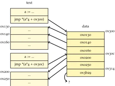
text a := ... jmp *(a*4+0x300) ... 0x130 ... 0x140 ... 0x160 a := ... jmp *(a*4+0x30c) ... 0x200 ... 0x250 data 0x0130 0x300 0x0140 0x0160 0x0200 0x30c 0x0250 0x3b29 0x314 ?
Figure4.1: Two jump tables in a program. As the value at address
31416 does not point into the text section, it does not
be-long to the jump table.
of basic blocks, i.e., we do nothing and split the functions later. Split points are then the destination addresses of call instructions.
4.1.4 Jump tables
Switch-case statement recovery is not a trivial task as pointed out by Cifuentes and Emmerik [12]. As there is already literature available,
we only describe how we recover jump tables. Jump tables are gener-ated when a switch-case statement has several successive numbered cases. The value of the control expression is used as index of the jump table. At the indexed position, an address into the code is found. The control flow is directed to this address by a jump instruction. Fig-ure 4.1 on the current page shows how the jump table looks in the
compiled program.
While we disassemble the binary, we need the destination address of the jump table to find all basic blocks. To simplify the detection, we interpret every computed jump as a jump table. It is possible due to our constraints on the input programs. In the computation, an address of the read-only data segment is involved; this address marks the start of the jump table.
To find the size of the jump table we need a data flow analysis. How-ever, it is not possible to do this analysis at the current time, as it needs information from a later phase. Therefore, we assume the size
of the table as big as possible. One limitation is the end of the data segment. The other limitation is not obvious. Every entry in the table points into the text segment since it is a jump destination. As soon as an entry does not point into the text segment we know that it does not belong to the table. With this method, we probably read too many entries. The superfluous ones can be removed in a later phase. This is a working algorithm, but there is much room for improvements.
4.1.5 Structuring
Our structuring algorithm uses a very narrow set of patterns. Since Java has labeled break and continue, they can also be used to get better code. In addition, fall through in the switch-case statement is not considered.
The problem of structuring is not new. Lichtblau [22], Cifuentes [11]
and Simon [28] provide more information for improvement of
struc-turing.
4.1.6 Stack variables
The simple method to detect stack variables, as illustrated in Figure
3.1on page10, is error prone. If an array is not only accessed by index
0 but also at other, constant indexes, our algorithm splits the array at those positions, too. We encountered cases where the compiler optimized in such a way that the only direct array access was at index
−1. In addition, the array size can be determined to be longer than used if the memory after the array is used for padding.
We expect better results with data flow analysis and range checks for dynamic arrays accesses. In addition, a way to use information provided by the user is necessary, since we do not expect perfect results for every input.
There exists literature about the topic; Chen et al. [9] propose a shadow
4.1.7 Library calls
Detecting library calls is necessary to properly link functions. A later translation of the library calls also depends on correct recognized library functions. Contrary to previous work by Cifuentes [11], it is
no longer a difficult problem when using ELF binaries with dynamic linked libraries on Linux.
To find the translation of addresses to function names, we use the same method as the dynamic linker does. A database provides fur-ther information about the library functions, such as the names and types of the arguments. Currently, the database entries are hand crafted. To some extent it should be possible to generate the database automatically from the header files of the libraries.
4.1.8 Tail calls
Tail call elimination is an optimization where the last function call in a function is replaced by a jump instruction. With this technique, there is no need to allocate an additional stack frame. There is no return instruction after the call statement, as the return of the function we jumped in is used.
A tail call is not a problem as the algorithm just follows the jumps. The called function is seen as part of the original function. If multiple functions “tail call” a function, the code of the callee is duplicated for every caller. It is not a problem with respect to correctness. The readability is higher when we detect such tail calls, but it can be part of the optimization as described in Section 5.2.3on page37. Further
work could be done to detect cases where code is duplicated, and extract that code into one function.
4.1.9 Aliasing of registers
To translate into SSA, we consider only flags and registers as variables as we do not have any information about aliasing of memory accesses. On x86, registers can be aliased, too, such asAL,AHandAXare part of EAX.
We implemented special rules to handle situations of register aliasing. Consider the case whenEAXis written and laterAHis read. The write
to EAX kills the registers AL, AH, AX and defines EAX. When reading
AHwe see that it is not defined butEAXis. Because we know that AH := ((EAX shr 8) and 0xff), we replace the access to AH with the expression((EAX shr 8) and 0xff).
4.1.10 SSA as intermediate representation
As described by Mycroft [25] and Emmerik [18], SSA has several
ben-efits in decompilation, such as simplified propagation or implicit use-def information. We see another important aspect of SSA. During compilation, many different variables are mapped to the same regis-ter. The variables are originally used because they express different things and moreover, they could have had different types. This infor-mation is lost as we only have a narrow set of registers without type information. If we transform the program into SSA, we decouple the various variables from the registers. Therefore, the only dependen-cies between variables are when they are assigned to each other, but not when they accidentally use the same register.
4.1.11 Coalescing unrelated variables
Coalescing has two effects. It reduces the number of used variables and the number of copy statements. The second is a consequence from the first as the merging of variables leads to assignments where the destination is the same variable as the source. So far it is the same as in a compiler. However, we have a different motivation for this phase.
For once, this optimization has non-functional reasons. Unlike in a compiler, we have arbitrary many variables we can use. We imple-mented it to make the code more readable.
Moreover, we do have additional constraints. Variables of different types are never allowed to be coalesced. In addition, we do not al-low coalescing of unrelated variables as we consider it as bad coding style.
For coalescing, we use the simple graph coloring method. Disallow-ing that two variables u andv are coalesced, means adding an edge between vertex u andv. Since we only allow coalescing of variables with the same type, we add edges from every variable to those vari-ables with different types.
We also want to prevent the coalescing of unrelated variables. To achieve this, we developed an algorithm to find additional constraints. The basic idea is, that we only allow coalescing of variables on the same data flow path. If they are on the same path, they are related. Our algorithm to build the constraint works as follows. First we build the data flow graph f. Then we build the transitive closuretof graph f and convert it to an undirected graph u. Figure 4.2 on page 31
shows an example for f andu. Finally the complementcofucontains the constraints needed to disallow coalescing of unrelated variables. Therefore, we add the edges fromc to the constraint graph used for graph coloring.
With this approach we get the desired results. Unrelated variables are not coalesced, even though it is allowed by the live ranges. Fur-thermore, it does not influence the number of copy statements. It is not possible as there is never an assignment of one of those variables to another one, since the variables are on separate data flow paths. Listing4.1on page31shows the results of our algorithm.
Nevertheless, there is still room for optimizations. Thus it can hap-pen, that a variable containing the size of an array, is used to count an index down. If we are able to decide the kind of the variables as described in Section5.2.3on page37, we can add more constraints.
4.1.12 Semantic gap
In contrast to Java, C and assembly code gives more control over the code to the programmer. Since this means that Java can not express everything we can find in a binary program, we need to address some issues.
We showed in our upcompiler how pointers can be handled by imple-menting an abstraction. However, pointers can be used in other ways we do not yet handle, i.e., cast parts of memory to different types. On the other hand, we think a direct translation of such cases does not result in good Java code.
Nevertheless, some specific constructs can be handled. Casting a floating point value to its bit representation can be done by the Java function Float.floatToIntBits. There are also functions for the other direction and for doubles. An array of bytes can be converted to and from an integer by basic mathematical operations. Java also provides methods to convert arrays of bytes into strings and back.
For memory blocks where we do not know anything about the con-tent, we should still be able to handle all cases. The memory is repre-sented by a memory stream class. This class has methods to access the data like the Java classes DataInputStream and DataOutputStream. In addition, seeking has to be possible. Accessing the stream class has to be abstracted by a pointer class, since different pointer variables have different positions in the memory. Unfortunately, this relies on the Unsafe API which is not standardized but widely supported. Unsigned data types have to be converted to signed types since Java does not yet have unsigned types, they are announced for JDK 8. If
the most significant bit is used too, the next bigger data type needs to be used. With theBigIntclass in Java, there is always a bigger data type available. Additional code may be inserted to ensure correct behavior for operations like subtraction.
It is possible that the upcompiler is not able to translate some pro-grams. We have some ideas to handle such cases. For example, parts or the whole program is executed in a virtual machine like JPC [6].
As it does not solve the upcompile problem, it opens the field for dynamic code analysis.
4.1.13 Obfuscation and optimization
Obfuscated binaries are actively changed in order to make it difficult to understand them. There exists tools and methods to obfuscate bi-naries, but we think the problem is more subtle. The compilation pro-cess itself destroys information contained in the source code. While compiling with no optimization and all debug symbols let you recon-struct most of the code, additional comments and other information is lost. Compilation with full optimization and no debug symbols makes the generated binary already hard to understand.
When a binary is actively obfuscated, it is hard to understand or de-compile it. Such techniques are used to protect the software against inspection. The reasons vary from enforcing of the copyright, pro-tecting trade secrets, propro-tecting against malware, protection against virus scanner and more.
Nevertheless, there is research going on. Kruegel et al. [21] and
Vi-gna [31] describe how obfuscated binaries can be read and analyzed.
But it is not done with the implementation of those methods in the upcompiler. The obfuscation will also affect other phases of the up-compiler.
Upcomiling legacy applications may be less challenging than new ones. Old compiler did less optimization or the optimization meth-ods are now better understood. On the other hand, software written decades ago may use techniques or patterns which are no longer seen as good practice. Such techniques include spaghetti code or extensive inline assembly.
Furthermore, obsolete processor architectures may led to different optimizations than modern ones. As a optimization is often bound to a specific hardware, understanding the hardware may be needed to understand the optimization. Reverting an optimization is more easy, if not crucial, when the optimization is well understood.
4.1.14 Functional programming languages
We assume that an upcompiler should be able to handle programs written in a functional programming language. Based on the Church-Turing thesis, for every algorithm written in a functional programing language an imperative version exists. If an upcompiler is complete, i.e., can handle the whole instruction set, it can upcompile every pro-gram.
Practically, we were not able to upcompile a Haskell program. A ma-jor problem is the huge size of the runtime system included in the compiled program. A “Hello World” program compiles into a 1.1
MiB binary, while the user code compiles into an 2.3 KiB object file.
With different tools we got a 199 line assembly file or 1702 line C
code. The runtime system consists of around 50,000 lines of highly
optimized C code. The tasks includes memory management, a par-allel garbage collector, thread management and scheduler, primitive operations for GHC and a bytecode interpreter [23].
Nevertheless, we think it is possible to adjust an upcompiler to func-tional programs. First, the user application has to be separated from the runtime system. For the runtime system, equivalent functionality has to be provided as Java code. We expect that rewriting is much simpler than upcompiling. For Haskell, this is true as the original code is available. The upcompiler only needs to handle the user code. It is possible that some parts of the user code is in bytecode. In this case, the upcompiler needs a front end for the bytecode or a bytecode interpreter is used during run time.
f u a b c d e f g h i a b c d e f g h i
Figure4.2: Data flow graph f of the program from Listing4.1on the
current page, and the undirected version of the transitive closure u of it. The components are not always complete. If two variables (vertices) are connected, coalescing those variables is allowed, hence the complement ofuis added to the constraint graph.
int main(){ a = readInt(); if(a > 0){ b = a; do{ c = b; d = c - 1; func0(d); b = d; }while(b > 0); func0(a); e = 0; do{ f = e; func0(f); g = f + 1; e = g; }while(e < a); h = 0; }else{ h = -1; } i = h; return i; } a b c d e f g h i a b c d e f g h i int main(){ a = readInt(); if(a > 0){ b = a; do{ b = b - 1; func0(b); }while(b > 0); func0(a); e = 0; do{ func0(e); e = e + 1; }while(e < a); h = 0; }else{ h = -1; } return h; } a b e h a b e h Listing4.1: Result of the constrained coalescing. Left is the program
before, right the same program after coalescing. The lines show the live ranges of the variables. Variable b, eand
hhave no overlapping live ranges. Due to our constraint for unrelated variables, they are not coalesced.
4.2 p e r f o r m a n c e
We measured the performance of the upcompiler as also upcompiled programs. All measurements were done on a computer with the fol-lowing specifications:
Processor Intel Core 2Duo CPU L9600at2.13GHz
Memory 1.7GiB
OS Ubuntu 12.04with Linux3.2,64-bit
LLVM 2.9
Java 1.6.0 24Sun Microsystems Inc.,64-Bit Server VM
4.2.1 Upcompiler
To measure the time of the phases, we instrumented the upcompiler. The numbers are the medians over16 measurements on 7 different
programs.
The most interesting numbers are the time spent in the different phases and the influence of the optimization level. Figure4.3 on the
following page shows both of them.
We see that the upcompiler performs best on unoptimized programs. Most of the differences in the time compared to the optimized pro-grams are in variable-handling related phases. Inspections of the unoptimized binaries have shown that the variables are mostly writ-ten back to memory. With this, the variables are preserved and the upcompiler hardly inserts phi nodes. In consequence, the upcom-piler does also not produce so many variables during SSA destruction which makes coalescing fast.
0 1 2 s optimization level 0 1 2 3 time in sec Others FunctionVariableLinker VariableReduction FunctionRecovery ArrayReplacer Disassembler
Figure4.3: Time spent in the different phases of the upcompiler.
4.2.2 Programs
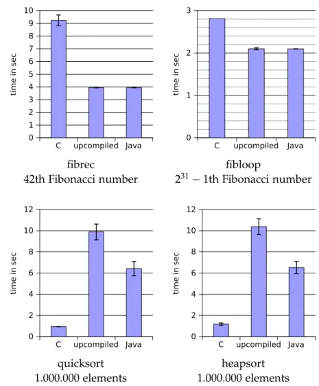
To determine the differences between compiled and upcompiled code, we measured the execution time of 4 programs. The first program, fibrec, calculates a user specified Fibonacci number in a very inef-ficient, recursive way. The second program, fibloop, has the same functionality but uses a loop to do it. Finally, we have a quicksort
and aheapsortprogram.
For every program we compare3versions. We have a binary version
compiled with optimization-O2, the upcompiled Java program, and a hand crafted Java version based on the C source. The changes for the last one are in order to make it Java compatible.
Figure4.4on the next page shows the median and standard deviation
over 10 measurements with same input for every program run. The
time is the user-time measured with thetimeutility. We try to explain some striking results.
The C version of the test programfibrecis more than2times slower
than the Java version. This huge difference is due to the fact that the recursive function is public and hence the compiler can optimize it only very conservatively. We declared the function private to test the hypothesis and measured an execution time of5.5seconds.
Since the upcompiled code of both Fibonacci programs is nearly the same as the C code, the similar times of the two versions are not surprising.
For both sorting algorithms, the upcompiled version is much slower than the Java version. In both cases the structuring algorithm failed for the compute-intense kernel function. The fallback mode is used there. We assume, this prevents Java from optimizing the code. The reasons for the difference between the C and Java version is not entirely known. We assume that the range checks on array accesses have a significant impact. Furthermore, the Java version spends a considerable time on tasks not related to sorting. We measured the sorting time of the hand written quicksort to be 3.0 seconds. This
does not include the start of the JVM, allocating memory, reading input or writing output.
C upcompiled Java 0 1 2 3 4 5 6 7 8 9 10 time in sec C upcompiled Java 0 1 2 3 time in sec fibrec fibloop
42th Fibonacci number 231−1th Fibonacci number
C upcompiled Java 0 2 4 6 8 10 12 time in sec C upcompiled Java 0 2 4 6 8 10 12 time in sec quicksort heapsort 1.000.000 elements 1.000.000 elements
Figure4.4: Performance comparison of upcompiled programs. We
compare an optimized C program, an upcompiled Java program and a hand written Java program based on the C code.
5
C O N C L U S I O N A N D F U T U R E W O R K
5.1 c o n c l u s i o n
We have demonstrated that upcompilation is possible by implement-ing an upcompiler. While it supports only a narrow set of input programs, we are able to fully and automatically translate those into Java source code.
Our upcompiler handles optimized32-bit x86 binary programs. The
binaries doe not need to have debug information or symbols. We detect calls to dynamically linked library functions and convert some of them to Java system calls. For the functions in the binary, we recover the local variables, arguments and return values. Memory accesses are converted to variables and arrays whenever possible. We convert the control flow graph to an abstract syntax tree, con-sisting of high-level language constructs. We type the variables to integer and pointer to integer. The upcompiler optimizes the code for readability. This includes expression reduction and code cleanup. Furthermore, we developed a custom coalescing algorithm in order to reduce the number of variables without merging unrelated vari-ables.
Since we implemented all phases, we touched all major areas in up-compilation. Within this thesis we describe the phases of our upcom-piler and describe the algorithms. The implementation can be found in the source code. We discuss problems we faced during implemen-tation. For some of them we present solutions, e.g., coalescing in the context of readability, detection of return values or the transforma-tion of stack memory to local variables. For the unsolved challenges, we present ideas or refer to available research literature.
We are aware that our upcompiler is not yet ready for real world applications. Since it is free software, we hope it is useful for others to study and/or extend it.
5.2 f u t u r e w o r k
A closer look at our upcompiler reveals that the binary is translated into a representation which is close to C and then wrapped into Java. It would be interesting to find a way to go directly to Java. However, since C is close to assembly, it may be difficult to do this.
We only analyze the code statically. If the upcompiler uses dynamic feedback, it can improve the code. Some conservative decisions may lead to slow execution or complicated source code. If the upcompiler has information from program runs, it is able to optimize the normal case. Such a dynamic method can be used on the original binary as well as in the produced Java source code.
The following sections describe problems we consider as most impor-tant for improving the overall result of the upcompiler.
5.2.1 Type recovery
The upcompiler only supports 32 bit signed integers and pointers
to them. For real world problems, this is clearly not good enough. Adding support for other primitive data types should not be a dif-ficult task. Already Cifuentes [11] describes how integer types with
more bits and unsigned integers can be detected.
Reconstruction of composite data-types like arrays, records or even objects is the the next step. We refer to other literature like Mycroft [25] and Dolgova and Chernov [17]. They describe the
reconstruc-tion of composite data types and give further references. Beside the static analysis, Slowinska et al. [29] describes how they use dynamic
analysis.
5.2.2 Generality
To widen the scope of input programs, the upcompiler needs several improvements.
We focused on binaries produced by LLVM, binaries from different compilers have to be tested. Support for more library functions is necessary and better support for printfand scanf, too. A broader range of input programs will also use more assembly instructions
than we support at the moment. Unusual composition, the use of inline assembly or code obfuscation tools also needs consideration. Furthermore, function pointers are not yet supported. They need special handling during upcompilation. The mapping to Java has to be implemented, too.
Improvements of the structuring phase together with SSA destruction could lead to better output. A switch-case reconstruction from jump tables is needed for more readable code. Better structuring leads to less cases where the fallback mode is used. A more sophisticated SSA destruction method may render coalescing obsolete or produces less copy statements in the final code.
Finally, support for more machines will improve the overall robust-ness of the methods. This is necessary because the goal of the up-comiler is to handle binaries of obsolete machines. Adding support for obsolete machines will be a recurring task.
5.2.3 Optimization and code metrics
The upcompiler has optimization phases like compilers have. As the optimizations of compilers can be measured in hard units, like exe-cution time or size of the produced code, there is no obvious metric for source code. Our coalescing phase has shown that reducing the number of variables improves the code quality, but there are more factors which have to be considered.
Obviously, it is difficult to write an optimizer without having a cost function. Literature about code metrics exists, we recommend Mc-Connell [24] as a starting point. In the remaining paragraphs, we will
discuss some optimizations.
The expression reduction we implemented is rudimentary, advanced code metrics are not considered. Our only consideration is, that we do not increase the number of expressions by copying them. This may improve the readability in a specific situation. But reducing all expressions as far as possible can reduce the readability if the expres-sion size becomes to big.
Loop recovery also improves the code readability. Transforming a do-while loop surrounded by an if statement into an do-while loop should reduce the complexity. Replacing while loops with for loops may also increases the readability.
Variable naming can directed by the kind of the variable. Iteration variables can be named as i, j and k, variables containing a size would be named n, m, size or count. Furthermore, name inference, e.g., using the names from library function arguments and propagate them, can significantly improve the naming quality.
For numeric values in the code, we propose a constant reconstruction. This means the replacement of numeric values by constants. If the same value is used multiple times, the same constant can be used if it has the same meaning. This can be decided with the same method as we use for coalescing. Naming the constants can be done as variables are named.
Function extraction reduces function sizes. It reverts the inlining from the compiler. The compiler can inline a function at several locations. With code clone detection [27] techniques we should be able to find
copied code. Nevertheless, we have to be able to find a good point where a function can be extracted. An extracted function should re-turn at most one variable and the number of arguments should be small.
A
B I B L I O G R A P H Y
[1] Boomerang. URLhttp://boomerang.sourceforge.net/. (Cited
on page4.)
[2] REC. URLhttp://www.backerstreet.com/rec/rec.htm. (Cited
on page4.)
[3] C2j. URL http://tech.novosoft-us.com/product_c2j.jsp.
(Cited on page4.)
[4] JGraphT. http://jgrapht.org/. (Cited on page5.)
[5] JSR 335: Lambda Expressions for the Java Programming
Lan-guage. URL http://jcp.org/en/jsr/detail?id=335. (Cited on page23.)
[6] JPC - The Pure Java x86PC Emulator.http://jpc.sourceforge. net,2009. (Cited on page29.)
[7] Brian Alliet and Adam Megacz. Complete Translation of Unsafe
Native Code to Safe Bytecode. InProceedings of the2004Workshop on Interpreters, Virtual Machines and Emulators, IVME ’04, pages 32–41, New York, NY, USA, 2004. ACM. ISBN 1-58113-909-8.
URL http://doi.acm.org/10.1145/1059579.1059589. (Cited on page4.)
[8] Gregory J. Chaitin, Marc A. Auslander, Ashok K. Chandra, John
Cocke, Martin E. Hopkins, and Peter W. Markstein. Regis-ter allocation via coloring. Computer Languages, 6(1):47 – 57, 1981. ISSN 0096-0551. URL http://www.sciencedirect.com/ science/article/pii/0096055181900485. (Cited on page19.)
[9] Gengbiao Chen, Zhuo Wang, Ruoyu Zhang, Kan Zhou, Shiqiu
Huang, Kangqi Ni, Zhengwei Qi, Kai Chen, and Haibing Guan. A Refined Decompiler to Generate C Code with High Readabil-ity. In Proceedings of the17th Working Conference on Reverse Engi-neering (WCRE), pages150–154, oct.2010. (Cited on page25.)
[10] Vitaly Chipounov and George Candea. Enabling Sophisticated
Analysis of x86 Binaries with RevGen. In Proceedings of the 7th
Workshop on Hot Topics in System Dependability (HotDep), 2011.