Forecasting and
Simulating Software
Development Projects
Effective Modeling of Kanban & Scrum
Projects using Monte-carlo Simulation
All rights reserved. FocusedObjective.com
ISBN: 1466454830 ISBN-13: 978-1466454835
CONTENTS
Acknowledgements... i
Preface ... iii
Why This Book Was Written ... iii
Who Should Read This Book ... iii
Chapter Outlines ... iv
Simulation and Forecasting Software used in this Book ... vii
Download the Simulation Software and Example Files ... vii
Chapter 1 ... 1
Modeling – Estimation, Forecasting and Risk Management ... 1
What is (numerical) modeling? ... 1
Just Enough Estimation ... 2
Choosing the right portfolio of projects ... 3
Planning, hiring and training staff for the future ... 4
Forecasting – Staff, dates, revenue and costs ... 5
Risk Management - Forecasting and avoiding disaster(s) ... 5
Managing Development Teams and Projects ... 7
Summary ... 8
Chapter 2 ... 9
Example Modeling and Forecasting Scenario ... 9
The Cast ... 9
Forecasting Staff and Dates – Getting the Go-Ahead ... 9
Act 1 – Backlog segmentation and Kanban Board Design ... 10
Act 2 – Cycle-time estimates ... 12
Act 3 – Staff tuning to bring in the date ... 12
Act 4 – Success; Getting to go-ahead ... 14
Hitting a Date Promised ... 15
Act 5 – Comparing Actual versus modeled ... 16
Act 6 – Rallying the Team to Reduce Defect Rates ... 17
Act 7 - What if we added staff now? ... 19
Act 8 - Impact (Sensitivity) Analysis ... 19
Project Retrospective ... 20
Summary ... 20
Chapter 3 ... 21
Introduction to Statistics and Random Number Generation ... 21
Summary Statistics ... 21
Minimum and Maximum... 21
Arithmetic Mean (or Standard Average) ... 22
Median ... 22
Mode ... 23
Standard Deviation ... 23
Percentile ... 24
Histograms ... 25
Interpreting Simulation Results Summary Statistics ... 25
Simulation XML Reports ... 25
Generating Random Numbers ... 28
Random Number Generators ... 28
Uniform Distribution ... 28
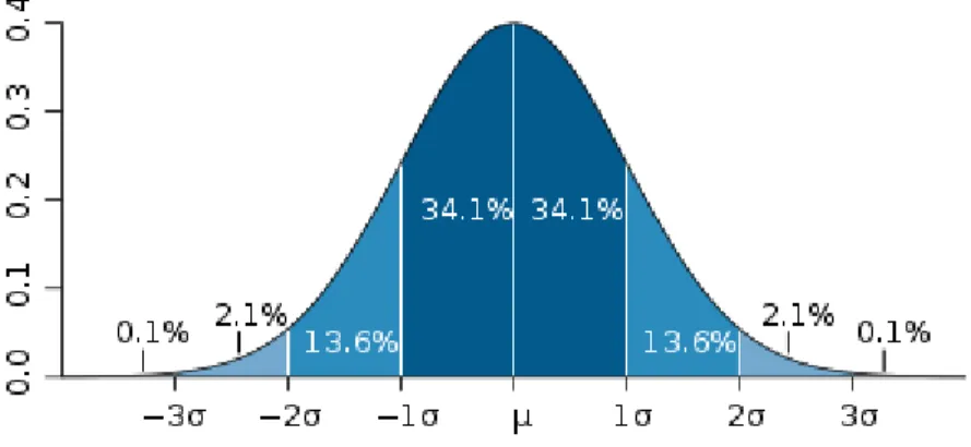
Normal Distribution (AKA Bell Curve) and the Central Limit Theorem ... 29
Skewed Distributions ... 31
Summary ... 33
Chapter 4 ... 35
Just Enough Estimation ... 35
Estimation Art ... 35
Estimating the 90th Percentile Range ... 36
Coaching Experts on 90th Percentile Estimation ... 36
Reducing the Amount of Estimation to a Minimum ... 41
Grouping by “Size” ... 41
Grouping by “Type” ... 42
Summary ... 44
Chapter 5 ... 45
Simulation Modeling Language Basics ... 45
Simulation Modeling Language – SimML ... 45
Simulation Section ... 46
Execute section ... 46
Setup Section ... 46
Example SimML Files ... 47
Lean/Kanban Modeling versus Agile/Scrum Modeling ... 49
Estimates in SimML ... 50
Making an Estimate Value Explicit (no range) ... 51
Backlog - Defining the work ... 51
Lean Percentage Cycle-Time Override ... 52
Lean Custom Column Cycle-Time Override ... 54
Agile Custom Backlog ... 56
Specifying Multiple Deliverables ... 57
Backlog Section Reference ... 57
Backlog section ... 58
Custom section ... 58
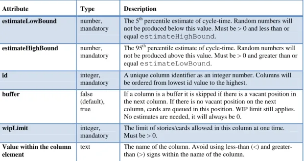
Column Section... 59
Deliverable Section ... 60
Columns – For Lean/Kanban Methodologies – The journey of work ... 60
Buffer and Queuing Columns ... 61
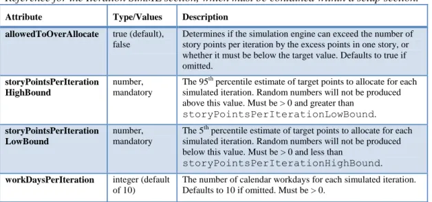
Iteration – For Agile/Iterative Methodologies – How much, how often ... 63
Summary ... 64
Chapter 6 ... 65
Modeling Development Events ... 65
Development Event Types ... 65
Event Occurrence Rates ... 65
Count Occurrence Rate– 1 in x Story Cards ... 66
Percentage Occurrence Rate – x% of story cards ... 67
Size Occurrence Rate – x story points ... 68
Making an Occurrence Rate an Explicit Value ... 68
Added Scope ... 69
Lean/Kanban Added Scope Events ... 69
Agile/Scrum Added Scope Events ... 70
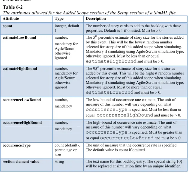
Added Scope Section Reference ... 71
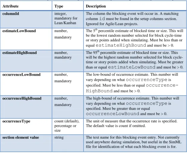
Blocking Events... 72
Lean/Kanban Blocking Events ... 73
Agile/Scrum Blocking Events ... 74
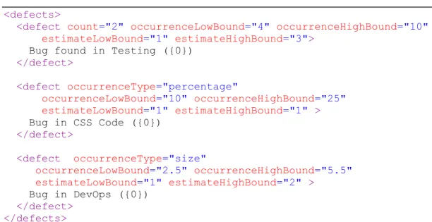
Blocking Event Section Reference ... 75
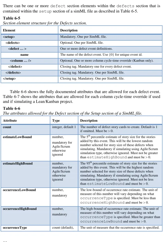
Defects ... 76
Lean/Kanban Defect Events ... 76
Agile/Scrum Defect Events ... 78
Defect Event Section Reference ... 80
Summary ... 81
Chapter 7 ... 83
Executing Simulations ... 83
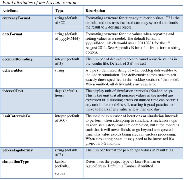
The Execute Section of a SimML File ... 84
Specifying What Deliverables to Simulate ... 85
Date formats ... 85
Running Simulations using the Kanban and Scrum Visualizer Application ... 86
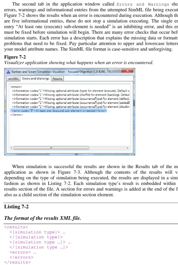
Visual Simulation ... 89
Creating Simulation Videos ... 90
Understanding the Visual Simulation XML Results ... 91
Kanban Visual XML Results ... 91
Scrum Visual XML Results ... 92
Monte-carlo Simulation ... 93
Summary ... 96
Chapter 8 ... 97
Forecasting Dates and Cost ... 97
Performing Forecast Date Simulations ... 97
Understanding the Forecast Date Results XML ... 99
Excluding Dates from Workdays ... 101
Summary ... 103
Chapter 9 ... 105
Analyzing Staff and WIP Limits ... 105
Staff Planning and WIP Limits ... 105
Performing Add Staff Simulations ... 106
Limiting the Columns Recommended ... 107
Understanding the Add Staff Analysis Results ... 108
Reducing Cycle-Time Simulation ... 111
Finding Kanban Board Balance ... 113
No More Developers Please – More QA & DevOps Staff! ... 114
Demonstrating More Staff Equals Less Project Cost ... 115
Summary ... 117
Chapter 10 ... 119
Sensitivity Analysis ... 119
Performing a Sensitivity Analysis ... 119
Understanding the Sensitivity Analysis Results ... 121
Proving Quality Code Counts ... 123
Summary ... 124
Chapter 11 ... 125
Analyzing Real-World (Actual) Data ... 125
Getting Actual Data ... 126
Iteration Story Points Range ... 126
Column Cycle-Times ... 127
Defect Occurrence Rates ... 128
Finding the 90th Percentile Range ... 129
Using Excel to Find the 90th Percentile Range ... 130
Using Kanban and Scrum Simulation Visualizer application ... 131
Summary ... 133
References ... 135
Appendices ... 136
Appendix A – Sample Model for Website Launch ... 136
Appendix B – Date Format String (dateFormat) ... 139
Acknowledgements
Although this book has a single author listed, its preparation was heavily influenced by many people, some of whom I want to call out specifically to acknowledge my gratitude.
Janet Magennis took the major workload of copy-editing my work. I’m prone to long rambling sentences that sometimes never completed; Janet fixed all of these and also my complete lack of consistency in punctuation and style day to day.
Daniel Vacanti is a thought-leader in the Kanban area and it has openly commented on his views about a more mathematical approach to managing software projects and how simulation can achieve the next level of maturity in our industry. He fielded the many a phone call when I wanted to run through some thoughts, and I thank him for his time and passion.
And although it seems cliché, I want to acknowledge you for buying this book. There needs to be more people taking the challenge of improving software project forecasting and management. By buying this book you have shown that you are open to new ideas and ways of working. I hope you send me some feedback and expand on this work by adding and publically discussing your own ideas on how to improve software forecasting.
Troy Magennis, Seattle. 2011.
Preface
Why This Book Was Written
This book was written because I believe that doubling a software project estimate should not be considered best practice. I’ve given, and been given estimates on software projects that I knew were wrong and misleading, and participated in doubling what I heard in order to account for “unknowns.” I knew there must be a better way and by researching other fields, I found and adapted techniques that make software project forecasting more accurate. These techniques embrace uncertainty and using it as a weapon against poorly considered project timelines and understaffed teams.
The process described in this book explains how to model software development projects, and to use those models to actively manage risk; for example, forecast dates, cost and staff requirements for a proposed project. Modeling and simulating a system provides a level of experimentation that is cost prohibitive to perform in practice. You don’t get to play out hundreds of what-if experiments on a real project – you get just one chance to deliver on-time and on-budget. The models we build represent a close facsimile of the real world software development process, the closer facsimile, the more accurate the results and better decisions made on interpreting those results – but as we will see, understanding the impact of each facet of the model helps us put the effort into improving the model (and project) only where that effort will give significant timeline improvement.
This book describes how to model the two most common methods for software development and delivery today, those being iterative based Agile processes based on story-point estimation (think Scrum), and lean processes that are cycle-time estimated (think Kanban). From a modeling and simulation perspective each offers opportunities for answering important questions. It is not the intention of this book to change your development process. Rather, I describe examples from both practices, however, some simulation types lend themselves better to one or the other, and I explain why when that occurs.
Who Should Read This Book
This book is intended for people in the software development industry who are looking for more certainty in the forecasting and staffing of their projects. Because this book also describes the benefit of modeling and what questions can be answered by simulating those models, this book will also be enlightening to executive management for software dev-elopment organizations.
People with the following responsibilities will find this book of interest – Project Managers: Understand how to model and forecast projects, and
how to simulate those models for answering questions regarding forecasting delivery dates, cost, and staffing needs.
Development Managers and Team Leads: Understand how to reduce the amount of estimation required for delivering forecasts, and how to determine what development events are causing the most impact to delivery.
Execute Leadership: Understand how multiple teams can co-ordinate their forecasts in a methodical way, and provide consistency in how these are generated and reported.
Venture Capital Investors: Understand how to obtain a reliable cost and date forecast for an investment as a primary or secondary opinion.
Chapter Outlines
Chapter 1 outlines the case for modeling and simulating software projects. The reasons why estimates are sought from management and the reasons these questions aren’t going away anytime soon.
Chapter 2 is an entertaining look at an example project scenario, demonstrating how modeling and simulation play a key role in from before projects get approved to the ongoing management of those projects. By the end of this chapter you will understand the end-game of simulation and modeling, and have a clearer picture of the answers achievable by using techniques described in this book.
Chapter 3 introduces the basics of statistics and random number theory that will be used throughout this book and your career in modeling and simulating software projects. The mathematics required isn’t complex, but the language and style of this book’s examples requires an agreed understanding and vocabulary to aid in digestion.
Chapter 4 discusses the estimation techniques required when building models. By utilizing modeling and simulation using the techniques described in this book, the amount of estimation is at its minimum necessary. This chapter describes how to quickly obtain the estimate ranges necessary from experts in systematic fashion to ensure accurate simulation and forecasts.
Chapter 5 introduces the simulation model language, SimML, and shows how to build your first Scrum and Kanban models. By the end of this chapter you will understand the basic structure of a model file, and know how to define the backlog of work and the project structure for Kanban and Scrum project types.
Chapter 6 describes the powerful event definition aspect to SimML models. It is the power of this eventing system that allows accurate simulation of the compounding impact of added scope, defects and blocking events on a forecasted date. Modeling these software project events is what makes building Excel spreadsheets difficult, and the reason SimML is so much more effective at representing real-world probability.
Chapter 7 shows how to simulate the SimML models. This chapter explains how to use the Kanban and Scrum Visualization application to perform visual simulation of a model for initial testing of the model and for showing others static or video demonstrations of the project simulated completion. This chapter also shows how to perform a Monte-carlo simulation of a model and interpret the results.
Chapter 8 is where all of the previous knowledge culminates in performing date and cost forecasts for modeled projects. This chapter explains how to perform forecasts and how to understand the results returned from the simulation engine.
Chapter 9 shows how to analyze the WIP limits and staff of a Kanban model. The staff analysis features of the simulation engine give recommendations of what Kanban column WIP limits to modify in order to reduce the cycle-time or completion time of a modeled system. This chapter gives example of how to find what skills the next hire should have, and how to present those suggestions to management in order to get the right resources on-boarded to complete your projects faster.
Chapter 10 shows how to perform impact analysis on a model. Impact or sensitivity analysis returns a list of what input factors cause the most change in forecast. Managing these most influential factors is the best use of your time, and lead you to make project changes and behavioral changes that most matter.
Chapter 11 looks at how to reverse engineer actual measured data. It shows how to determine if measuring and mining certain data is value for money, and once you determine that a certain measurement is important, how to analyze that data to update the values in your model for more accuracy.
Thank you for being interested in improving the software development process, and I hope you find the journey of modeling and simulating a fulfilling one; one that gets you answers to the questions you have quickly and accurately.
Simulation and Forecasting
Software used in this Book
In order to run the examples shown throughout this book you need to download and install the Focused Objective Kanban and Scrum Simulation Visualizer application. As a purchaser of this book you qualify for a free license to experiment and follow along with the examples in this book on your own.
The features of this software are –
Simulation engine that supports Agile/Scrum projects and Lean/Kanban projects.
Simulation engine that supports visual (video’s), Monte-carlo, forecasting date and cost, and sensitivity analysis commands.
Model editing application that color codes and groups model code. Visual simulation result application window to single-step through a
project one day or iteration at a time.
XML and HTML format reporting for simulation results.
Summary statistics application that helps reverse engineer existing data for improving model inputs.
Download the Simulation Software and Example Files
The simulation software setup application can be downloaded from –
http://www.focusedobjective.com
The instructions found at this location include system requirements, and how to download and install the application.
Chapter 1
Modeling – Estimation,
Forecasting and Risk
Management
To set the scene for the rest of the book, this chapter outlines the reasons for and why modeling and simulating software projects is necessary and important. The answers a model can provide go far beyond improved timeline estimates. The ability to quickly test alternative project backlog and staffing structures, and the ability to uncover what factors are most influencing the forecasted results makes modeling critical to success. Modeling is the first step to actively managing all aspects of development process through experimentation via numbers.
What is (numerical) modeling?
Modeling is the art of building an artificial version of an object or process for the purpose of experimentation. Modeling provides a cheaper way to measure the impact of various factors and determine the utility of an object or process without completing that project first. In our case, modeling provides a level of certainty around forecasts of time to complete, the resources required and cost.
A model serves the purpose of understanding the interplay between its various input factors. Determining what factors, and what level of input is required for those factors to cause an artificial failure to occur (an undesirable result, in our case – too long a time or too much cost). Once the model is built, it can be used to predict future outcomes. For example, a *very* simplistic model of a software project is –
Work days to complete =
(Estimated days of work / number of developers) + ((Estimated days of work * Defect rate) /
number of developers)
In this example model, the input values of estimated days of work, the number of developers, and a defect rate multiplier (in this model, 0.5 would mean 50% of the work again to account for defects) are combined to forecast the number of workdays. Each input variable has a role to play and impacts the output value. For example, adding developers decreases the result, increasing the defect rate makes the number of days to complete longer. For even this simplest of model, good conversations can be had on the subjects of
resourcing and how to decrease defect rates. When this model is expanded to cover more real world occurrences like scope-creep, testing, release management, vacation time, developer skill levels, etc. the model is capable of answering even more complex questions.
Throughout this book, we refer to a model as a tool to allow various analyses to occur on a software development project or portfolio. For the model to work effectively, it needs to be fed enough information to approximate the real world process being mimicked. Many of these input values cannot be fully known in advance, and estimates must be provided; the techniques in this book minimize the need for exact measure by insisting that the likely range (lowest likely, and highest likely) be provided in their place. This allows the model to equate the most likely, with some variation both below and above the most frequent result.
For the moment, think of a model as a mathematical formula. It combines various input values and provides a result. Changing the inputs changes the result. And if one of the inputs isn’t known, the formula can be rearranged with a hard-coded result argument in order to solve what that unknown value could be. The ability to continuously perform what-if scenarios in very short time frames is where a model offers a level of understanding of a system far in excess of human intuition (albeit expert opinion) alone.
This book describes how models of software development projects and portfolios can be quickly built and simulated. The results of these simulated “project completions” are assessed in a variety of ways in order to understand and forecast the most likely future outcomes (and some you wish you had never uncovered). It all starts with those important input values which have to be estimated – the single word that strikes fear and loathing into every developer’s psyche. Let’s cover the broad need for estimation in more detail.
Just Enough Estimation
It is common for estimation to be deemed a waste of time by many participants in the software development process. I have to agree that when playing the role as a developer, I had an adverse opinion as to the need of delaying the start of a project, or stopping the project in order to carry out “another” round of estimation. However, as I made my way into executive management of IT teams and departments, I saw another side to estimates, the one that gets projects approved, and the right number of staff hired. Our aim should always be to do the least amount of estimation possible, and this book describes techniques that get to accurate forecasts with the least amount of estimation distress, arriving at a solution with a desired level of confidence quickly in order for important decisions to occur. I encourage you to keep an open mind on the subject of “estimates are waste” until you see later in this book the types of answers and management techniques possible with just a few estimates.
There are multiple reasons estimation is still important, and this chapter explores the basics of a couple of the major drivers –
1. Choosing the right portfolio of projects, and getting the go-ahead. 2. Planning, hiring and training staff for the future.
Choosing the right portfolio of projects
Most companies don’t have a single project idea to build, and even if they do, there is a variety of features and differing opinions as to what features are critical in order to go to market. Choosing which projects get completed and in what order is an important aspect of executive management, but in order to effectively perform this task, these people need some information in which to make decisions.
In larger organizations, the necessity for yearly budgeting is the catalyst for causing all the business stakeholders to present ideas that will allow that company to hit revenue targets in the following year. Sometimes this process is ongoing, with ideas and innovations presented to an “innovation council,” at regular times, and those elected on that council to give the nod of approval. All of these approaches for a company managing its new project work require two basic bits of information for each initiative – 1) How much revenue will it make, and 2) How much will it cost. The goal is to understand if the investment being made will reap reward in an acceptable timeframe, often referred to as Return on Investment or ROI. The Return on Investment formula is at its most basic–
Return on Investment = Revenue – Cost to develop
Revenue (and therefore ROI) is time sensitive, meaning the earlier a feature is in the market earning revenue, the higher the total revenue for the next calendar period. Knowing when a project will be delivered, earning customer revenue is critical to understanding how much cash a given initiative will add to the following years bottom-line. This means that for any considered investment decision, a reliable calendar date estimate of when that feature or innovation will be ready to earn income is necessary, and that is one reason we are constantly asked as developers and program managers to give a delivery date (another being to calculate the cost to develop).
Stepping into your investor shoes for a moment– if you were getting your kitchen remodeled, you would likely want an up-front estimate (and certainly from more than one) vendor in order to make a buy decision. Very few major investments in life occur with the buyer not getting a cost estimate. And software development should be added to that list. I fully understand the concept of Agile getting features to market incrementally, bringing the return on investment earlier, but when needing to make a go/no-go decision and to choose between multiple options- an estimate of the costs involved is necessary before work starts. The return on investment is going to be necessary to ensure that the right projects get started – the projects that improve the bottom line the most.
If the development team isn’t given the task to estimate an idea, or are unwilling to do so, SOMEONE ELSE will do it for them. I can’t stress this point enough, being proactive in getting the business estimates is key to NOT having someone else form an opinion of how long you will take to do your work. Nobody wants that to occur, but if you had to choose from a portfolio of fifty ideas, and cull them down to ten that will get the go-ahead for the next year (and form the basis of staffing and budget allocation), you would need to know the cost side of the equation.
Another disturbing trend that can cause the wrong projects to progress through the investment phase is the continual doubling of estimates. After being asked for an estimate, it’s not uncommon for the person presenting those estimates to add a buffer, a clumsy and often random approach to managing risk. This means that in some cases, the cost of a very
minor change, balloons into a major project; or a well estimated initiative gets shelved due to the perceived excessive cost. Doubling the value given is a common approach, and whilst this might bring poorly estimated projects into a more real-world estimate, I’d prefer to improve the estimation process, rather than just accept it as flawed and make an in-accurate estimate more in-in-accurate. I’ve seen the doubling approach cause major loss of trust between the business folks and the IT department through ludicrous doubling on doubling of numbers making a minor change a three-month project (the project manager doubled the developer estimate, and the business owner doubled all estimates again when they rolled up all projects – nothing gets approved).
The real goal of estimation is to arrive at an estimate, within an agreed accuracy, in as short a time and minimal staff disruption as possible. This is where modeling and simulating a project is key, and the purpose of the remainder of this book.
Planning, hiring and training staff for the future
Another area where estimation occurs is planning staffing levels for the future. There are always exceptions, but most companies need to match the size of their teams to the amount of work forecast for the future period. Some of this team is required to maintain business as usual, and some of the team is for new features and products, and some of this team is overhead – people required for the organization to continue operation.
The number of staff maintaining business as usual might be thought of as static; but even existing products go through phases of updates, or are impacted by traffic growth that might require remediation work. Somebody has to match supply and demand of these resources, and ensure that the right capacity is available for both the current and future plans. Sometimes future product plans require new skills to be introduced, and making sure the current staff up-skill ready to meet those demands is an important part of being an effective manager. To manage this process, an understanding of the throughput capacity of the team, and the impact of the upcoming tasks on that team needs to be continuously estimated and managed.
Having a model of the team and its throughput is the first step in understanding the hiring needs when demand exceeds supply. Quickly being positioned to know how many and what skills are needed to hire is one of the key management skills required to be effective long-term in the software industry.
When evaluating new projects, the ability to model and provide a resourcing plan is the key element in providing a cost budget. Salary or external contracting costs traditionally are the biggest cost in a software development project. Turning developer estimates into a resource plan that achieves a desired delivery date is the essential element for the cost side of the return on investment equation (as mentioned in the choosing the right portfolio of projects section previously).
Building a resource plan isn’t just the number of developers. Designers, testers, operations and release staff are only a few of the other team members required to deliver any software. The resource plan has to match the supply for each area of expertise with the demand for the project, and scale the team in order to bring delivery into a desired date range. For example, a project might define three feature teams (three parallel teams to do work); on each feature team there would be a designer, three developers and a tester. To release the product earlier, a decision might be to add an additional feature team – five people. Finding the right balance will be very project and team member experience
dependent. Modeling that team and using simulation to determine the correct balance and impact of adding more staff is a key technique explained now and expanded on later in this book (see Chapter 9).
Forecasting – Staff, dates, revenue and costs
Forecasting is calculating in advance the condition or occurrence of some aspect – in the case of software development, most commonly staff, delivery date, cost and revenue. Estimation plays a role in understanding magnitude of each element, but forecasting combines these many elements into a single unit of measure; either time, or money (or both). Reliable forecasting requires understanding the factors influencing a final result, and accounting for each of them with educated estimates. The more factors you miss, the less accurate (or uncertain) the forecast. When as many as practical factors are combined using estimates for a software project and modeled, the simulation output can be relied upon to give accurate forecasts.
Turning a software feature estimate (or set of estimates) into a delivery date is one forecasting example. Knowing the starting date, the teams size and structure, and the number of days to design, build, test and release a feature allows us to calculate a delivery “live” date. However, more factors are at play, for example, accounting for public holidays, fixed release date windows, a third party delivering a new logo-design, are just some additional factors that might impact the forecast date. In the end, for managing the ROI calculation, nobody cares deeply about the estimate – it’s the forecast that really matters
(but to get to the forecast we need the estimate), and the forecast combines all factors rolling up the results to a final cost or date.
Calculating the move from estimates to a forecast quickly gets complex, and beyond the human scope to solve intuitively (although we try). The interplay between factors, and the flow-on impact of small events early in a project cause major shifts in release date and costs. This gives the illusion that it’s a problem too hard to reliably solve, but the process is more understood than first thought. Tools and techniques are available that solve similarly hard problems in other domains, and this book describes an approach using custom tools built for the purpose of forecasting software development projects.
Accurate forecasting is possible and necessary. This book describes the techniques for achieving accurate forecast of software deliver and cost, and how to use those forecasts in decision making.
Risk Management - Forecasting and avoiding disaster(s)
Forecasting has a level of uncertainty. Any forecast does, just ask any meteorologist you might know and sympathize with them; they must get cornered at every party gathering and hounded by those assembled as to why they get the forecast wrong so often. Weather forecasting tries to model mother-nature, and apply current observations with historical trends to predict the future state of environmental climate. Software doesn’t get impacted by natural events (mostly – baring the occasional natural disaster like earthquake or flooding of the server room), although some events that occur seem wildly random. For the
most part, there are a finite number of events and those events have a range of possible values with fairly narrow upper and lower bounds. In essence, forecasting software delivery is much easier than weather, and we should continue to get better at both. Just like weather forecasting, the closer to the date being forecast, the more likely an accurate result. Both types of forecasting incur greater uncertainty as the time horizon is extended due to the ripple and knock-on effect of early variations in inputs. To reliably model software development (and weather), the model must embrace and simulate how early events combine and influence the longer term results.
Risk management can be broadly defined as the identification, assessment, and prioritization of risks followed up by managing and monitoring those risks in a project (Wikipedia). I also like the definition given in the ISO 31000 standard as “the effect of uncertainty on objectives, whether positive or negative”. For our purposes, managing the estimate and forecast risk so that better decisions are made on project we are involved is another plausible definition. It is our job to include risks in our modeling of software projects and to always clearly state the uncertainty of our forecasts so that other people can manage and monitor their risks, and make more informed decisions.
The uncertainty of a model is the range of outputs for a forecast when the input estimates are at their combined worst or combined best. Different levels of uncertainty are appropriate at different times – in portfolio planning, an estimate plus or minus one month might be okay when comparing a few options. However, this range of uncertainty is a deal-breaker to the plan if the cost of failure (not meeting a date for instance that causes missing a legal requirement and incurring fines) is excessive. Risk has a common index equation that helps assess and prioritize the most impactful, most probably risk events first –
Composite Risk Index = Impact of event x Probability of Occurrence This formula works simply by getting participants to identify potential risk events, and then allocate a 1 to 5 point value to both the impact (1 = low impact, 5 = major impact) and occurrence probability (1 = very unlikely, 5 = almost certain). These values are multiplied together and the results sorted highest to lowest, assisting in prioritizing the most likely and the most impactful risks to those first managed. I believe this method whilst better than none at all is a far cry from what is possible and necessary, and I’m not alone. Douglas Hubbard in his un-diplomatic book, The Failure of Risk Management: Why It's Broken and How to Fix It (Hubbard, 2009), presents a passionate argument that most methods for managing risk are less than useless and actually cause harm, likening them to “no better than Astrology.” He goes onto describe scientific, quantative methods to manage risk, such as Monte-carlo simulation that this book and the tools it describes are based. I obviously agree with his findings, and whilst not wanting to go to the extreme to recommend disbanding any current risk management program relating to software development (or other endeavor), I do recommend understanding and applying the risk management methods describe throughout this book – primarily, modeling and simulating a system.
Modeling and simulating a system doesn’t directly estimate a risk index. Once a model is produced, it is possible to directly simulate the impact of one risk occurrence versus another and compare that to all other risks. For example, it may not be clear upfront what the impact is of losing a certain number of staff members, or what the impact is of outsourcing one particular skillset. With a model of the software development process, it is possible to simulate both occurrences and compare that to a baseline simulation forecast on
cost and deliver date. The results of this experiment will yield more powerful information in which to make a decision as to how much effort to invest in avoiding (or embracing) those events or strategies. Traditional risk management might highlight an event, whereas modeling and simulation highlight and give magnitude and levity to an event.
Later in this book we carefully look at how to find what factors most influence a forecast, a process called sensitivity analysis. Putting you in the position to constantly know and manage the most impactful elements in a system (in this case a software product or portfolio) is a key goal and purpose of this book and the techniques and tools it describes. I know it sounds like nirvana and a pipe dream at the moment, but the techniques are proven and frequently used in other adventurous fields (finance and mineral exploration for example).
Managing Development Teams and Projects
Good managers set clear goals for their teams. Clear goals are shared ambitions that a manager puts in place by describing the need, the solution and a way to know if progress towards hitting that target solution is being made. A shared vision is a starting point, and too often, team members don’t have access to, or don’t get visibility into the underlying reasons for a certain goal.
Modeling a system allows impact to be demonstrated, proven and therefore communicated earnestly to staff. Factors impacting the forecast can be identified and managed early if the actual occurrence rates or size are in excess of that initially modeled. Reality will diverge from the model from time-to-time, and in these cases, the model is the starting point to a necessary conversation. In some cases, the model needs changing, but this is a fact to be celebrated! If the change has significant impact on one of the promised forecasts, action can be taken earlier. This divergence also makes the next model more accurate, and these lessons foster an environment of true understand of the entire software development system as a whole – meaning fewer surprises occur in future projects.
The ability to demonstrate that one aspect of the model is having a greater impact than another helps change team behavior. For example, when seeing that a certain type of production defect (say, development environment URL’s being promoted to production) is the highest hitter on a sensitivity analysis (a simulation that ranks what inputs have the most influence on a forecast), the team can quickly grasp that it isn’t just management inventing problems to solve, the simulated model based on real-world occurrence rates is demonstrating a clear massive impact on a final delivery date. It is often abstract for all team members to be on the same page with respect to how such little problems cascade and grow into weeks or months of delay, but with a model, it can be shown to them. Once understood by the team, setting a target of halving the occurrence rate by the next iteration is a much easier sell.
When using the techniques described in this book, I’ve found managing my team-leads more effective. Our one on ones are often looking at the model, comparing actual data (occurrence rates and estimates of blocking issues and defects), and discussing any departure. Once we identify a significant departure of model from reality, we agree on whether the model needs to be changed, or the departure managed by the team to bring it back into the model’s range. These meetings are some of the most productive meetings I
have had (and I hate meetings), Often I walked away learning more about my teams and the factors faced by my development organization than days of retrospectives.
Modeling and simulation offer an opportunity to connect and influence your teams in ways that are non-confrontational and productive. This book describes the techniques to model a system development process and then by comparing actual measured data, identify problems, find solutions and then set targets to make hitting forecasts the most likely outcome.
Summary
This chapter outlined the reasons for modeling and what the benefit is for all team and management members. The answers a model provides go far beyond improved timeline estimates. A model helps all stakeholders understand the impact of their field of expertise and influence on others. Uncovering what factors are most influencing cost, revenue recognition, staffing size and delays, is the first step to actively managing those aspects to hit a goal.
Chapter 2
Example Modeling and
Forecasting Scenario
This scenario is for a hypothetical project that aims to re-launch a website. It demonstrates the thinking process and practical implementation of using modeling to quickly forecast staffing levels, go-live dates, and how to interact with senior management to get good decisions made. At the moment, you may not understand all of the terminology and the software used to generate the reports; we cover this material later in the book. This scenario is one of any number of ways of estimating, modeling and forecasting a software project. It’s meant to spark your creativity.
The Cast
You – You have the job of managing a team to produce and re-launch the next generation website that will save “The Company.”
Charlie – Your CTO. He holds the keys to the budget for staffing requests.
Boris – Your business owner. He has the grand vision and the ear of the CEO.
Your Team – A group of Graphic designers, web developers, server-side developers and testers. At the moment, the exact number of resources you need isn’t clear. You have a core group already consisting of -
1 – Graphic Designer 2 – Web Developers 3 – Java Developers 1 - QA Engineer
Forecasting Staff and Dates – Getting the Go-Ahead
Your project is one of three options for next year’s budget the CEO is considering. He likes all of them and has asked for a better view on the cost of development and the delivery forecasts. The CEO wants a new website to go live before the end of the calendar year. Rumors are your major competitor has a new site to launch end of Q1 next year, and the CEO wants to beat them to it. He also wants to limit investment to $250K in labor costs.
You need to get a cost and delivery date forecast quickly to answer these questions. The first step is to gather the information needed without disrupting the development teams current project. You need to quickly generate the following numbers –
1. Staffing estimate in order to hit at least a partial deliverable by end of calendar year
2. Cost estimate to deliver (forecast)
3. Probability of hitting certain dates (forecast) Note:
Appendix A is listing of the full SimML model file.
Act 1 – Backlog segmentation and Kanban Board Design
To begin, you need a backlog of work to model and estimate. Reviewing the initial backlog of 31 stories you have been given, and roughly modeling defects and blocking events using occurrence data from prior projects, you run a quick forecast date simulation with a very basic Kanban board definition and cycle-time estimates (as shown in Figure 2-1). You want to see how close to January 1st the most basic of simulation model gets you.
Figure 2-1
Basic starting point for Kanban board and estimation.
You execute a forecast date simulation run for 31 backlog stories. Listing 2-1 shows the SimML code that performs a Monte-carlo simulation and extrapolates the completion date, and likelihood percentage of hitting that date, and a simple cost estimate (simple estimate ($100K / 52 / 5) x number of staff, now 7). The results of this simulation are shown in Output 2-1.
Listing 2-1
SimML command to run a forecast date simulation.
<execute deliverables="Must-Haves" dateFormat="ddMMMyyyy"> <forecastDate startDate="01Oct2011" intervalsToOneDay="1" workDays="monday,tuesday,wednesday,thursday,friday"
costPerDay="2700" /> </execute>
Output 2-1 clearly shows you have your work cut-out for you to deliver by the beginning of the year, and the cost is high, your target is around $250K. At the moment, you only feel confident in saying March 1st, which is approximately your 95th percentile result.
Graphic-Design (wip limit 1) •cycle-time •low bound: 1 •upper bound: 3 UI-Code (wip limit 2) •cycle-time •low bound: 1 •upper bound: 3 Server-side-Code (wip limit 3) •cycle-time •low bound: 1 •upper bound: 3 QA (wip limit 1) •cycle-time •low bound: 1 •upper bound: 3
Output 2-1
Most basic simulation of 31 stories using default column cycle-time.
<forecastDate startDate="01Oct2011" intervalsToOneDay="1" workdays="monday,tuesday,wednesday,thursday,friday" costPerDay="2700" ><dates>
<date intervals="96" date="13Feb2012"
likelihood="1.60 %" cost="$259,200.00" /> …… removed from brevity ……
<date intervals="108" date="29Feb2012"
likelihood="92.00 %" cost="$291,600.00" /> <date intervals="109" date="01Mar2012"
likelihood="94.80 %" cost="$294,300.00" /> <date intervals="110" date="02Mar2012"
likelihood="98.40 %" cost="$297,000.00" /> <date intervals="111" date="05Mar2012"
likelihood="99.20 %" cost="$299,700.00" /> <date intervals="112" date="06Mar2012"
likelihood="99.60 %" cost="$302,400.00" /> <date intervals="113" date="07Mar2012"
likelihood="100.00 %" cost="$305,100.00" /> </dates>
</forecastDate>
You work with Boris, and segment the backlog into two deliverables: Must-Haves, and Everything-Remaining. You then work with your developers and partition each group further. You make a fast pass through the stories and put them into one of four categories-
1. Small: Those stories that are possibly under a days work, but certainly less than 2 days work in each column.
2. Medium: Those stories that are more than 2 days work but less than 3 days. 3. UI-Intensive: Those stories where lots of graphics design and UI coding is
necessary.
4. Server-Side-Intensive: Those stories where lots of Java service (or .NET, we are all friends here) code is required.
Table 2-1
Estimates grouped by deliverable and then by size and skill specialty. Delivery Group
Must-haves
Developer Estimate Group Number of Stories
Small 6
Medium 4
UI-Intensive 5
Everything-remaining
Developer Estimate Group Number of Stories
Small 2
Medium 3
UI-Intensive 2
Server-side Intensive 3
Act 2 – Cycle-time estimates
For each of the story categories you ask the development team to come up with 90th percentile ranges for cycle time, meaning the cycle-time they feel the actual cycle-time is between the range they give (5% below, 5% above). The final model for Kanban columns and the cycle-times is shown in Figure 2-2.
Figure 2-2
Final Kanban columns, Wip limits and cycle-time estimates for the backlog groups
With this story partitioning, and estimated cycle-times for each category of story in each Kanban column, you look at the forecast for just the “Must-Have” group.
<date intervals="83" date="25Jan2012"
likelihood="94.80 %" cost="$224,100.00" /> <date intervals="84" date="26Jan2012"
likelihood="96.80 %" cost="$226,800.00" />
Act 3 – Staff tuning to bring in the date
You are still beyond the target date needed to get a go-ahead. You must find what extra staff will bring that date into range. You perform a staff sensitivity simulation on the model (called the addStaff command in SimML) and find what it recommends. Listing 2-2 shows the SimML command to determine what the best three column WIP limit changes have the most impact.
Graphic-Design (wip limit 1) •small cycle-time: •1 to 2.3 days •medium cycle-time: •1.6 to 3 days •UI-Intensive : •2 to 5 days •Server-side-intensive: •1 to 3 days UI-Code (wip limit 2) •small cycle-time: •1 to 2.3 days •medium cycle-time: •1.6 to 3 days •UI-Intensive : •3 to 5 days •Server-side-intensive: •1 to 3 days Server-side-Code (wip limit 3) •small cycle-time: •1 to 2.3 days •medium cycle-time: •1.6 to 3 days •UI-Intensive : •1 to 3 days •Server-side-intensive: •3 to 6 days QA (wip limit 1) •small cycle-time: •1 to 2.3 days •medium cycle-time: •1.6 to 3 days •UI-Intensive : •1 to 3 days •Server-side-intensive: •1 to 3 days
Listing 2-2
SimML command to find what staff additions make the most impact to delivery
time. In this case, 3 staff recommendations will be made, and every Kanban
column can be changed.
<addStaff count="3" cycles="250" />
The addStaff simulation makes three recommendations, add a Graphics Designer, a QA engineer and then a UI Coder in that order. The recommendations are cumulative, and you notice that there is only a marginal benefit in adding the UI coder which is an expensive resource, so you decide not to add that resource. This simulation expected a 34% improvement (reduction) in intervals (days for this simulation).
Output 2-2
Results table for staff simulation. Improvements are cumulative, and
improvement is over the original baseline.
WIP Suggestion Graphics-Design by 1 the QA by 1 then UI-Code by 1
Original WIP 1 1 2 New WIP 2 2 3 Intervals to completion (original 78 intervals) 72 51 47 Cumulative Interval Improvement 7.3% 34.95% 40.68%
Figure 2-3
Simulation chart for recommendations of adding 3 people. Days to completion drop from 78, to 72, to 51, to 47.
Act 4 – Success; Getting to go-ahead
With the results from Output 2-2 and Figure 2-3 you re-run the forecast date simulation with increased column WIP’s for Graphics Design and QA. In order to forecast the extra cost, you must increase the per day cost burn rate by 2 staff as well (using the same formula as before ($100K / 52 / 5) x number of staff, now 9). You present your findings to Charlie (the CTO) and get the approval to borrow a designer and add a QA engineer if your project gets the go-ahead.
Listing 2-3
SimML command for forecasting completion date with extra resources, and an
increase in per-day cost to account for funding those resources.
<forecastDate cycles="250" startDate="01Oct2011" intervalsToOneDay="1"
workDays="monday,tuesday,wednesday,thursday,friday" costPerDay="3461" />
By simulating the SimML command as shown in Listing 2-3, it is now possible to hit the end-of-year target with just the Must-Haves (a scenario Boris supports) with a very high degree of certainty as shown in Output 2-3.
Output 2-3
Forecast date estimate with the extra staff accounted for. This is for the
Must-Haves ONLY. You can deliver before end-of year.
<date intervals="54" date="15Dec2011"
likelihood="94.00 %" cost="$186,894.00" /> <date intervals="55" date="16Dec2011"
likelihood="95.60 %" cost="$190,355.00" /> <date intervals="56" date="19Dec2011"
likelihood="98.40 %" cost="$193,816.00" /> <date intervals="57" date="20Dec2011"
likelihood="100.00 %" cost="$197,277.00" />
To deliver the entire project, you also feel confident in delivering by mid-January, and the total cost of very close to the $250K investment target as shown in Output 2-4.
Output 2-4
Forecast date estimate with the extra staff accounted for. This is for the entire
project. Cost is now in-line with expectations.
<date intervals="72" date="10Jan2012"
likelihood="94.00 %" cost="$249,192.00" /> <date intervals="73" date="11Jan2012"
likelihood="97.20 %" cost="$252,653.00" /> <date intervals="74" date="12Jan2012"
likelihood="98.80 %" cost="$256,114.00" /> <date intervals="75" date="13Jan2012"
likelihood="100.00 %" cost="$259,575.00" />
Boris and Charlie present the business case to the CEO. The CEO is pleasantly surprised that not only did you hit the targets he asked for; he can see that there was method to the calculations and trusts that you can manage to those numbers. Your project gets the go ahead.
From the developers’ perspective, they gave a total of 4 estimates of cycle-time, and a single pass through the backlog categorizing the work. They thank you for not having to estimate all 31 stories, and then re-estimate them again when the target wasn’t achieved.
Hitting a Date Promised
The project has now been underway, and ten stories have been completed. It’s time to make sure that your project is tracking to the model by comparing actual data versus the model’s estimates.
Act 5 – Comparing Actual versus modeled
After the first month and a half, actual data can and should be used to refine the cycle-time estimates. The original estimates were very wide in order to capture the group’s consensus quickly on what the 90th percentile range would be. Now with a number of stories completed, with a variety of things that went well, and things that went wrong, a narrower range is likely to emerge.
The first step of analyzing actual data is to confirm that the actuals fell within the ranges estimated for cycle-time. Table 2-1 lists the cycle times estimated by the developers, and as you can see in Table 2-2 there were three actuals that fell outside of that range. A 5% variance above or below the range expected for 40 samples would be 2 stories above and 2 stories below; the actuals are showing 2 cards above, which is on the line, but within the bounds, and 1 card below, which is also below the 5% limit. It is too early to be making changes, but keeping an eye on the Medium category time is in order, another cycle-time above the limit would mean you should increase the cycle-cycle-times for simulation. Table 2-2
Actual column cycle-times for the project after the first 10 stories. 3 cells fell outside of the range estimated.
Cycle-Time Actuals
Story Delivery Group
Dev. Estimate Group Graphics Design
UI Code Server Side Code
QA
Story 1 Must-Haves Small 2.21 0.97 1.22 2.13
Story 2 Must-Haves UI-Intensive 4.28 4.11 1.23 1.31 Story 3 Must-Haves Medium 2.26 0.89 1.39 1.73 Story 4 Must-Haves UI-Intensive 2.47 3.77 1.22 1.38 Story 5 Must-Haves Server-Side-Intensive 1.84 1.99 5.30 1.93
Story 6 Must-Haves Small 1.34 1.24 1.34 1.44
Story 7 Must-Haves Server-Side-Intensive 1.99 1.85 5.08 2.36
Story 8 Must-Haves Small 1.78 3.08 1.77 1.63
Story 9 Must-Haves UI-Intensive 3.91 3.24 1.63 1.50 Story 10 Must-Haves Medium 2.37 1.66 1.83 1.71
Defect rates and blocking event rates do not look as promising. The original estimates in the model compared to actual are shown in Table 2-3. UI Defects are occurring every story. This is twice the rate expected, and is impacting the delivery date.
Table 2-3
Defect and blocking event estimate versus actual occurrence rates after 10 stories. Occurrence Estimate Occurrence Actual
UI Defect 1 in 2 to 3 stories 1 in 1 (10 so far out of 10 stories) Server-side Defect 1 in 3 to 6 stories 1 in 5 (2 so far out of 10 stories) Block Spec Question 1 in 5 to 10 stories 1 in 3 (3 so far out of 10 stories) Block Testing Environment 1 in 4 to 8 stories 1 in 5 (2 so far out of 10 stories)
Act 6 – Rallying the Team to Reduce Defect Rates
When you initially modeled your project, you took the defect rates and the blocking event rates from a previous project. You have identified by comparing actual data on this project that one of your defect types, specifically UI related defects is occurring more often than you modeled.
Listing 2-4
SimML model for the UI Defect definition where actual occurrence is once in
every story.
<!-- Originally modeled UI defects, found in QA, fixed in UI Dev-->
<defect columnId="4" startsInColumnId="2"
occurrenceLowBound="2" occurrenceHighBound="3">UI Defect </defect>
<!-- New model based on actual occurrence rates -->
<defect columnId="4" startsInColumnId="2"
occurrenceLowBound="1" occurrenceHighBound="1">UI Defect </defect>
You update your model definition for this defect from once in every 2 to 3 stories to once every 1 story, matching the actual measured occurrence rate you are seeing from the project. Running a date forecast simulation using this new definition for the Must Haves delivery group shows you will miss the end of year target as shown in Output 2-5.
Output 2-5
New date forecast showing the impact of the UI Defects.
<date intervals="66" date="02Jan2012"likelihood="93.20 %" cost="$228,426.00" /> <date intervals="67" date="03Jan2012"
likelihood="97.60 %" cost="$231,887.00" /> <date intervals="68" date="04Jan2012"
likelihood="98.40 %" cost="$235,348.00" /> <date intervals="69" date="05Jan2012"
likelihood="99.60 %" cost="$238,809.00" /> <date intervals="71" date="09Jan2012"
likelihood="100.00 %" cost="$245,731.00" />
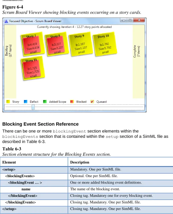
You pull your team together and explain the observation of UI defects. You share the new date forecast and show them the visual video simulation of the Kanban flow as seen in Figure 2-4.
Figure 2-4
Video screenshot of simulation showing the team the impact of the defects on throughput.
You then demonstrate that adding a full day to the cycle-time of every story in the UI-Code column has less impact than the UI Defects currently are causing (as shown in Output 2-6).
Output 2-6
Impacts of increasing the cycle-time for UI-Dev by 1 day (lower and upper
bounds). Less than the impact of UI Defects alone!
<date intervals="62" date="27Dec2011"
likelihood="94.40 %" cost="$214,582.00" /> <date intervals="63" date="28Dec2011"
likelihood="96.80 %" cost="$218,043.00" /> <date intervals="64" date="29Dec2011"
likelihood="99.60 %" cost="$221,504.00" /> <date intervals="66" date="02Jan2012"
likelihood="100.00 %" cost="$228,426.00" />
On seeing and understanding the impact of these defects, the team brainstorms ideas on how to bring the occurrence rate back into the once every 2 to 3 stories. Their ideas of giving the business owner (Boris) a demonstration and feedback before checking in, getting a peer-review, and spending an extra half-day testing the stories themselves are effective and occurrence rates return to those expected over the next few stories.
Note
Being able to show that working slower and more carefully (by not allowing defects to be raised in later columns) WILL reduce the
overall project time is a key lesson. Although most of this scenario is contrived, this lesson isn’t – spend an extra half a day testing during development, as this case shows, even if you spent a day testing you would still be better off than allowing the UI defect rate be high.
Act 7 - What if we added staff now?
Charlie the CTO in your weekly meeting asks you if you want more staff to make sure you reach the promised delivery date. He offers as many developers as you need. You perform an add staff simulation (results shown in Output 2-7), and demonstrate that whilst adding one UI Developer would be the most benefit right now, an additional Graphics Designer and QA Engineer are then next in line most beneficial to throughput.
Output 2-7
The results of an addStaff SimML command showing the next three staff
additions that have most impact on reducing days of work.
<wipSuggestion column="UI-Code" originalWip="2" newWip="3" intervalImprovement="9.45" >
<wipSuggestion column="Graphics-Design" originalWip="2" newWip="3" intervalImprovement="14.78">
<wipSuggestion column="QA" originalWip="2" newWip="3" intervalImprovement="22.26" >
He assigns another UI Developer to your team, and lets you borrow a graphic designer from another team who is ramping down on another project.
Note
I’ve been around a few projects that underwent scrutiny for being late. The upper-management reflex was to offer and add
developers, but it rarely works. The ability to show that just adding developers without increasing the capacity surrounding them is a waste of time is invaluable.
Act 8 - Impact (Sensitivity) Analysis
You want to see what most impacts the delivery date; is it the defects or the blocking events? Your graphics designer is complaining about the business being slow to respond to questions. You want to see if that would impact your delivery date by a meaningful amount. You perform a sensitivity analysis on the SimML model.
A sensitivity report gives you an ordered list of what input factors of the model change the delivery date the most. When managing a project it’s good to know what factors to go-after and solve next, and a sensitivity reports makes your next opportunity clear. Listing 2-5 shows how to perform a sensitivity simulation.
Listing 2-5
SimML command to execute a sensitivity report. Returns an ordered list of what
most influences the output.
<sensitivity cycles="250" sortOrder="descending"
estimateMultiplier="0.5" occurenceMultiplier="2" />
The sensitivity analysis is enlightening (Table 2-4) for the development team. It shows that even if the occurrence rate for the specification questions was halved, it would make less than a single day difference to the final outcome. UI Defects remains the highest impacting defect. The development team stops complaining about the lack of response to questions and you get to re-iterate the importance of limiting the UI Defect occurrence rate. Table 2-4
The results from executing a sensitivity analysis on the model UI Defect Spec question
(awaiting answer) Spec question (awaiting answer) Block testing (environment down) Block testing (environment down) Server-Side Defect Object Type
Defect BlockingEvent BlockingEvent BlockingEvent BlockingEvent Defect
Change Type
Occurence Estimate Occurrence Estimate Occurence Occurence
Interval Delta
-3.344 -0.812 -0.744 -0.468 -0.328 -0.248
Project Retrospective
Although it was tight, the addition of a UI coder, a Graphics Designer and a QA Engineer helped quickly resolve some last minute defects and change of scope that Boris and his team wanted after seeing the completed site. The Must-Have features were delivered before the New Year, in mid-December. The Everything-Else delivery group was completed early in the New Year and the extra features helped raise considerable revenue leading up to and over the Christmas and New Year season.
From your perspective, you felt you always had a clear picture of what needed to be managed, and early indications of issues that might risk delivery date promises. Charlie, your boss was also impressed that for every meeting you came prepared with a list of impacting events (a sensitivity report), and knew what staff additions would have the most impact.
Summary
Although this was just a fictional scenario (or was it?) you can quickly see how the use of a model and simulation tools can quickly give you the ability to understand impact of various what-if questions, and the confidence to ask for what you need.
Chapter 3
Introduction to Statistics and
Random Number Generation
This book requires a basic level of mathematical ability. When modeling IT projects, we rarely get beyond the basic mathematical operators of plus, minus, multiply and divide – but we do need to understand the terminology of how large groups of numbers are summarized and investigated, a field called Statistics.
The first part of this chapter introduces the statistical terms you need to understand the model and interpret the results of simulations performed later in this book. The second part discusses the intricacies of random number generation. Random numbers play a pivotal role when modeling a process. Random numbers are used as inputs to a model in order to simulate a result, and how these random number inputs are produced and the patterns used can make a model accurately reflect outcomes, or be completely useless.
Statistics 101
Statistics is defined as the mathematics of the collection, organization, and interpretation of numerical data (The Free Dictionary). For the purposes of this book, we use statistics to make sense of the results from a simulation performed over a model of the software development process. Rather than present thousands of numbers, the reports generated for us by the simulation tools described later in this book are summaries of that data using statistical terminology, often called summary statistics. This section refreshes our memory of the mathematical and statistical terms and definitions so that there is no confusion when explaining the examples later in this book.
Summary Statistics
When dealing with large sets of numbers, there are a few important summary statistic measures used to represent different aspects of that set of numbers. We will cover each of these in this section.
Minimum and Maximum
From a large set of numbers, there will be a value that is the lowest value, and a value that will be the highest. There is no limit to the extents that a value is bounded, it will be one of the members of the set of numbers, and if that set has only one member, that minimum and maximum can be the same value. Minimum and maximum has no relationship to zero;