Epidemiologic Perspectives on Drunk Driving

(1)

35

Epidemiology and Data Management

Epidemiologic

Perspectives on

Drunk Driving

M.W. Perrine

Vermont Alcohol Research Center, Burlington, Vermont Raymond C. Peck

Research and Development Office

California Department of Mot& Vehicles, Sacramento, California James C. Fell

National Centerfor Statistics andAnalysis, National Highway Tmfic Safety A&n&istration, Washington, D. C.

What is the one element found in approximately half the U.S. highway fatalities? This

question has been raised over the last few decades and the answer is still the same: Alcohol. This answer generates another question: If a single, identifiable element is involved in such a large portion of a serious public health and public safety problem, should it not receive top priority for investigation, in’tervention, and prevention?

Alcohol produces both pleasure and pain, euphoria and depression. Alcohol also

produces many jobs and billions of dollars in tax revenues to the States and to the Nation. Each year, alcohol also produces unintentional death to thousands and injury to millions. When mixed with driving, alcohol is the basis for a major public health and public safety

problem. In our automotive society, the car is used for almost all facets of social activity.

Therefore, since alcohol is involved in many aspects of social behavior, driving after drinking is a relatively frequent occurrence. Fortunately, the vast majority of such driving-after-drinking instances do not result in crashes. One very important task for researchers is to identify variables that differentiate between those driving-after-drinking instances that do result in a crash and those that do not.

How do we learn about the contribution of alcohol to unintentional injury and death on the highways? In attempting to do so, we still find a large gap between description and explanation that, at this time, can be bridged only provisionally through inference. Two widely separated research approaches have been used to date as a basis for inferring the contribution of alcohol to highway crashes: epidemiologic and experimental.

NOTE: Primary responsibility forparts of this chapter is as follows: J.C Fell, the subsection entitled “Alcohol fnvolvement in Fatal Highway Crashes”; RC. Peck, the subsection entitled Tharactersitics of Drunk Dfiw-s”; M.W. Perrine, all other sections. The first author is grateful to Robert B. Voas for early discussions of this chapter and for material p&i&d in the sections on “Other Roadside Research” and “Enforcement Checkpoints.” Preparation of M.W. Perrine’s part of this chapter and production of the manuscript were supported by PHS Research Grants .4,474, AA06926, and AA07876 from the National Institute on Alcohol Abuse and Alcoholism.

(2)

36 BACKGROUND PAPERS

The epidemiology of alcohol and highway safety can be traced from the first review of the problem presented in 1933 (Miles 1934). Over the years, high blood alcohol concentration (BAC) has &en thoroughly implicatedin serious and fatal injury highway

crashes by post hoc epidemiologic studies. Most evidence for relating-this alcohol contribution to highway crashes has been obtained by examination of the distribution of BAC both among drivers involved in actual crashes (fatal and nonfatal) and- on the basis of case-control roadside surveys-among drivers using the highways, but not involved in crashes at the time. A number of such case-control studies have demonstrated that alcohol is overrepresented among deceased drivers relative to drivers in the population-at-risk using the highways at corresponding times and places (e.g., Borkenstein et ‘al. 1964, 1974; Perrine et al. 1971; for reviews see NRC 1987; NHTSA 1985; Perrine

197%; b).

The second approach consists of controlled administration of alcohol in experiments conducted on isolated variables that are assumed to be relevant for actual driving. Alcohol impairment of real-world driving performance is then typically inferred from the mosaic of these bits of behavior examined separately in the laboratory, in driving simulators, and in instrumented cars driven on closed courses (NRC 1987).

Both research approaches to the study of drunk driving are necessary and have been productive (NRC 1987; Perrine 1976). However, this chapter is limited to epidemiologic aspects; it is organized as follows:

A discussion of the scope of the drunk-driving problem from an epidemiologic perspective

A brief outline of the major components involved in studying the problem by means of the available data sources

A review of the most relevant literature, focusing on alcohol involvement in fatal as well as nonfatal highway crashes and in noncrash drivers; crash risk and alcohol; and characteristics of drunk drivers

An examination of current issues and problems

Scope of the Problem

The primary problem clearly consists of those motor vehicle crashes that result in fatal injuries. It is now generally well established that alcohol is involved in approximately half of all such fatal crashes. For example, the total number of highway fatalities in 1986 was 46,056, of which some 24,000 (52 percent) involved alcohol. More specifically, BACs exceeded the typical legal limit (0.10) in 41 percent of all fatal crashes.

An estimated 4.8 percent of deaths in the United States during 1980 were directly or indirectly attributable to alcohol (NIAAA 1987). Of these, motor vehicle crashes were the largest single cause of death. Approximately 26,000 deaths in 1980 were attributed to alcohol in motor vehicle crashes; these deaths constituted about 27 percent of the total number of deaths (approximately 98,000) attributable to alcohol (NIAAA 1987, p.6). The number of alcohol-involved motor vehicle deaths is about two times that of the second largest single cause of alcohol-involved death, namely, homicide (approximately 12,000 or 12 percent) (NIAA4 1987, p-6).

The scope of the alcohol and traffic safety problem has recently been reviewed briefly both from a public health perspective (NIAAA 1982,1985,1987) and from a public safety perspective (NHTSA 1985,1987b; NRC 1987). In this chapter, the problem is examined further to provide a more integrated synthesis of the literature from both these perspectives.

(3)

EPIDEMIOLOGY AND DATA MANAGEMENT

Major

Components

of the Study

37

Aside from epidemiologic methodology considerations, the major components involved in the present perspective on drunk driving consist of the data sources. The two primary sources of data for this area are offtcial records and surveys of various types.

The official records consist primarily of the following:

The citation report for driving under the influence of alcohol (DUI) The accident report, if alcohol is involved

The prosecutor record Court records

Department of Motor Vehicle records Treatment/service provider records Probation department records

Of special importance are those reports of accidents in which a fatality resulted, since these data are collected at the State level and then forwarded to the Fatal Accident Reporting System (FARS) of the National Highway Traffic Safety Administration (NHTSA). As an example of using such data, analyses of DUI processing from the point of the arrest citation through the other official records, including the postconviction countermeasures, have been prepared for the State of California (Perrine 19&1; Helander 1986; Peck 1987).

The other major source of data for epidemiologic studies consists of surveys. The main varieties are:

roadside surveys,

telephone surveys (in recent years, the random-digit-dialing telephone SuNeY),

household surveys, and

special location surveys (bars, jails, etc.).

Of these various types, only the roadside surveys can obtain direct measurements of the major criterion variable- namely, BAC- from drivers actually using the roads at the time. All the other survey methods depend on self-reported information from the respondents, including data concerning driving after drinking. Thus, only the direct measurement of BAC at roadside can be used to provide criterion measures for estimating alcohol crash risk and for evaluating the impact of countermeasure programs on the motoring public.

Review of the Most Relevant Literature

Alcohol Involvement in Fatal Highway Crashes

In 1986, 46,056 people were killed in traffic crashes (NHTSA 1988), which are the leading cause of death for Americans age 6-34 (Richardson 1985). Traffic fatalities in 1986 resulted in 1,425,517 years of potential life lost before age 65, an amount greater than deaths from cancer, heart disease, and all other causes. Traffic crashes cost society approximately $74 billion annually in terms of damage, insurance costs, injury treat- ments, lost work, and so forth. (NHTSA 1987c). Since 1900, over 2,600,OOO Americans have died in traffic crashes; that is 1,500,OOO more than the total number of Americans killed in all the wars in U.S. history.

(4)

It is well known that ‘alcohol is a leading factor in traflic crashes. It was involved in over half of thetraffic fatalities in 1986, resulting in close to 24,000 deaths (NHTSA 1988). Each year, nearly 560,000 additional people suffer injuries in alcohoi-related crashes - an average of one person injured every minute of the day. About 43,000 of these injuries are serious (NHTSA 1988).

During the 198286 period, approximately, 119,000 people lost their lives in alcohol- related traffic crashes-an average of one alcohol-related fatality every 22 minutes over the past 5 years. About two out of five Americans will be involved in an alcohol-related crash in their lifetime (NHTSA 1987u). Approximately 1800,000 drivers were arrested in 1986 for DUI - an arrest rate of about 1 out of every 90 licensed drivers in the United States (Greenfield 1988).

The problem is especially devastating for young people. In 1986, more than 40 percent of all teenage deaths resulted from motor vehicle crashes. Over half of these were alcohol related, making alcohol-related traflic crashes the leading cause of death for teenagers. For traffic crash victims age 20-24, close to 70 percent of the 8,000 who died in 1986 were in alcohol-related crashes (NHTSA 1988). The probability that a given death is due to a traffic fatality is 55 times as great for a ul-year-old male as for a 65year-old male; the corresponding ratio for females is 43 (Evans 1987).

The average BAC of drinking drivers involved in fatal crashes was 0.15 in 1986 (NI-ITSA 1985). The legal intoxication limit in most States is 0.10. In a recent survey of drivers jailed for drunk driving offenses, over a quarter of the drivers had consumed at least 20 beers or 13 mixed drinks within 3-4 hours before they were arrested (Greenfield 1988). Research has shown that a driver with a BAC of 0.15 has a 26times greater probability of beii involved in a crash than a sober driver (NHTSA 1985).

FARS indicated that 41 percent of the traffic fatalities in 1986 involved either a driver or a pedestrian with a BAC of 0.10 or greater. This percentage translated to 18,890 fatalities. An additional 11 percent (5,100 fatalities) involved a driver or pedestrian with some alcohol (BAC = 0.01-0.09). Only 48 percent of the fatalities involved all drivers and pedestrians with zero alcohol.

Alcohol involvement did vary by time of day, day of week, and type of crash (table 1). Seventy-seven percent of the fatal crashes that occurred between 8 p.m. and 4 a.m. on any night of the week involved alcohol. Alcohol was also much more prevalent in single-vehicle crashes than multiple-vehicle crashes. Almost half the collisions resulting Table 1. Alcohol involvement in fatal crashes: 1988

Crashes BAC 0.01-0.09 0.10 and higher N (pzznt) (percent) (percent) Fatal Daytime (4 a.m. - 8 p.m.) Nighttime (8 p.m. - 4 a.m.) Weekday

Weekend (8 a.m. Fri - 4 a.m. Mon) Single vehicle Multivehicle Nonoccupant (pedestrian/bicyclist) 41,062 48 11 41 23,828 67 9 25 16,900 23 14 63 22,700 59 9 32 16,277 35 12 53 17,114 38 11 51 16,244 58 11 - 31 7,704 51 9 40

(5)

Table 2. Drivers and nonoccupsnts (pedestrians/bicyclists) involved in fsul crsshes: 1986

BAC

39

0.00 0.014.09 0.10 and higher N (percent) (percent) (percent) - All drivers 60,297 66 8 26 Driver fatalities 26,613 52 9 39 surviving drivers 33,684 77 8 15 Nonoccupant fatalities 7,770 64 7 29 Male drivers 46,622 63 9 223 Female drivers G734 79 6 15

in a nonoccupant (pedestrian or pedalcyclist) death involved alcohol, mostly on the part of the pedestrian.

When examining data for all drivers involved in fatal crashes, keep in mind that in multiple-vehicle crashes, at least two drivers are involved in one crash. In 1986,60,297 drivers were involved in the 41,067 fatal crashes. Twenty-six percent of these drivers were legally intoxicated (BAC greater than or equal to 0.10) at the time of their crashes (table 2). Of the 26,613 drivers who were killed in their crashes, 39 percent were legally intoxicated compared with only 15 percent of the drivers who survived fatal crashes. Male drivers were almost twice as likely to have over 0.10 BAC at the time of their crashes as female drivers (28 percent versus I.5 percent).

Alcohol involvement did vary substantially by driver age in 1986 (table 3). While 21 percent of teenage drivers were legally intoxicated at the time of the crash, an additional 13 percent had also been drinking. Drivers 28-24 years old had the highest alcohol involvement rate: 47 percent. In contrast, only 7 percent of drivers age 65 and older were legally intoxicated at the time of their crash.

Examining certain combinations revealed that while almost two-thirds of the fatal Table 3. Alcohol involvement by driver age, 1986

Driver’s BAC

Driver’s age 0.00

(percent)

O.Ol-.09 0.10 and higher

(percent) (percent) N* 16-19 66 13 21 7,854 20-24 53 12 35 11,427 25-34 59 8 33 16,163 35-54 72 6 22 14,305 55-64 81 5 14 4,017 65 and older ₈₉ 4 7 4,881 All ages 66 8 26 60,297

(6)

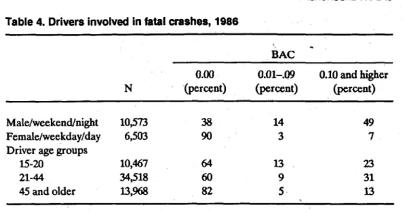
Table 4. Drivers involved in fatal crashes, 1986

iAC - N O.Ol-.09 (percent) 0.10 and higher (percent) Male/weekend/night 10273 38 14 49 Female/weekday/day 6,503 90 3 7

Driver age groups

15-20 10,467 64 13 23

21-44 34,518 60 9 31

45 and older W@ 82 5. 13

crashes involving a male driver on a weekend night were alcohol related, only 10 percent of the crashes involving a female driver in a weekday crash in the daytime involved alcohol (table 4).

Alcohol involvement was also found to vary considerably by the type of vehicle driven (indicating the type of driver, in most cases) (table 5). Drivers of motorcycles involved in fatal crashes had by far the highest alcohol involvement rate: 54 percent. Only 3 percent of heavy-truck drivers involved in fatal crashes had BACs over 0.10. Drivers of older vehicles were more often legally intoxicated than drivers of newer vehicles (34 percent versus 22 percent).

Intoxicated drivers in fatal crashes also tended not to use safety belts. Of the fatally injured drivers who were at zero alcohol, 20 percent were wearing safety belts compared with only 7 percent of. the fatally injured drunk drivers. Thirty-six percent of the zero-alcohol surviving drivers were reported as using belts, in contrast to only I.5 percent of the intoxicated surviving drivers.

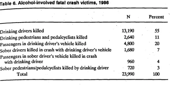
Contrary to some popular misconceptions, the victims of alcohol-related fatal crashes are most often the drinking driver or drinking pedestrian. Two-thirds (66 percent) of the 23,990 victims of alcohol-related crashes in 1986 were the drinking driver or driig pedestrian (table 6). An additional 28 percent of the victims were passengers in the Table 5. Drivers involved in fafal crashes, 1986

BAC

Drivers of: 0.00 0.01-0.09 0.10 and higher

N (percent) (percent) (percent)

Motorcycles 4,542 46 I.3

Passenger cars 35,920 65 9

Light trucks and vans 11,724 63 8 29

Medium trucks 653 92 3 5

Heavy trucks 4,355 95 2 3

Older vehicles (older than 1976) 13,168 59 9 34

(7)

EPIDEMIOLOGY AND DATA MANAGEMENT 41

Table 6. Alcohol-involved fatal crash victims, 1986

N Percent ’

Drinking drivers killed 13,190 55

Drinking pedestrians and pedalcyclists killed 2pJ 11 Passengers in drinking driver’s vehicle killed 4,800 20 Sober drivers killed in crash with drinking driver’s vehicle 1,680 7 Passengers in sober driver’s vehicle killed in crash

with driiig driver 960 4

Sober pedestrians/pedalcyclists kiied by drinking driver 720 3

Total =,=J 100

drinking driver’s vehicle. Additional analyses revealed that in fatal crashes where BACs were known for drivers and their passengers, 36 percent of the time the driver was legally intoxicated but the passenger was not.

Table 7 shows the basic trend with regard to the alcohol problem in fatal crashes over the past 5 years. The percentage of drivers in fatal crashes who were intoxicated (BAC = 0.10 or greater) at the time of the crash decreased from 30 percent in 1982 to 26 percent in 1986-a Gpercent reduction, which is substantial. The reduction was especially great for teenage drivers (table 8). While 29 percent of the teenage drivers in 1982 were legally intoxicated, this amount dropped to 21 percent in 1986, a 28percent reduction. While this teenage driver trend is encouraging, one must still keep in mind that teenage driver involvement in fatal crashes per mile driven is substantially higher than other driver age groups (Fell 1987). .

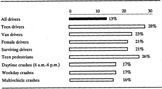
The nature of this S-year alcohol reduction trend was examined in the following manner. Specific decreases of certain types of drivers and certain types of crashes were compared with the overall reduction. If these specific reductions were substantially greater than the overall reduction, then that would indicate that these drivers or conditions were affected most, Figure 1 summarizes the key fmdings concerning the nature of the reduction.

The largest reductions noted were for teenage drivers (28 percent), followed by teenage pedestrians killed in collisions (26 percent). Also affected were drivers of vans (23 percent reduction), female drivers (21 percent), and drivers who survived the fatal Table 7. BACs for all drivers involved in fatal crashes, 1982-86

(in percents) BAC 1982 1983 1984 1985 1986

198246

change

0.00 ₆₁ ₆₂ ₆₄ 66 66 0.01-0.09 9 9 9 8. 8 0.10 and higher 30 29 27 26 26 -14 N _{56,029 54,656 57,512 57,883 60,297}

(8)

Table 8. BACS for teenage (l&19) drivers Involved in fatal crashes

BAC 1982 (m percents) _\ - 1983 1984 1985 1986 198286 change 0.00 58 61 6% 67 .66 0.01-0.09 13 13 13 11 13 0.10% and higher 29 27 24 -22 21 -28 N‘ 7,467 7,050 7,366 7,151 7,854

crashes (17 percent). The absolute reduction was also larger in weekday crashes (17 percent) and in multivehicle crashes (16 percent).

Drivers age 25-34 had only a slight reduction during this S-year period (6 percent). Motorcycle drivers, with the highest percentage of alcohol involvement to begin with, experienced no change in the percentage of drivers legally intoxicated during this period. Pedestrians age 20-64 also had no reduction in the percentage legally intoxicated between 1982 and 1986. Late night crashes and single-vehicle crashes showed only modest reductions in the percentage of drivers who were at 0.10 BAC or higher (6 percent and 9 percent, respectively).

The average BAC of drinking drivers in fatal crashes in States where most of the drivers were tested showed a modest decrease from 0.165 in 1980 to 0.153 in 1986.

Alcohol consumption per capita decreased in the United States between 1982 and 1986. But if that decrease was a prime factor in the decreased alcohol involvement of drivers in fatal crashes, then a similar reduction should have occurred in intoxicated adult pedestrians in fatal crashes, which was not the case.

All drivers 0 10 20 30 -13% Teen drivers Van drivers I -1 28% 1 123% Female drivers I t 21% Surviving drivers II 21% Teen pedestrians

r

126%

Daytime crashes (6 a.m.-6 p.m.) I : 1 17%

Weekday crashes Multivehicle crashes

I ... 1 17%

B 1 16%

Figure 1. Nature of alcohol reduction in fatal crashes, 1982-88 Decrease in percentage drunk (BAC = 0.10 or higher)

(9)

EplDEMlOLOGY AND DATA MANAGEMENT

Table 9. Nature Of alcohol reduction among fatally injured &iv- with known BACs in 15 good reporting states*

(percents)

43

BAC of fatally 1980 1981 1982 1983 1984 l985 1986 l980-86

injured drivers change

00 39 40 41 43 46 49 48 +23

.01-m 11 11 11 10 11 10 12 +9

m-.19 27 26 25 25 23 22 22 -19

.20+ 24 23 23 21 m 19 18 -25

-

*Test and report BACs on 85 percent of fatal drivers.

The nature of the reduction of alcohol in fatal crashes does seem to point to main effects in responsible social drinkers, i.e., substantial reductions in daytime crashes, by female drivers, drivers of vans, and teenagers. However, there is some evidence that the percentage of drivers with very high BACs is also decreasing, at least in the 15 “good- reporting” States in FARS. Table 9 shows that, in 1980, almost a quarter (24 percent) of the fatally injured drivers in these States had BACs of 0.20 or greater. That portion in 1986 was 18 percent, which was a 25-percent reduction-greater than the reduction for the drivers at BACs between 0.10 and 0.19. Most researchers would agree that drivers at 0.20 BAC or greater are most likely problem drinkers or alcoholics. Yet the percentage of drivers at these levels has decreased significantly since 1980 (in that l5-State sample). Are these problem drinkers finding alternatives to driving? Are they confining their drinking to their homes? Have many of them stopped drinking? More research is necessary to answer these important questions.

Alcohol in Noncrash Drivers

Accurate determination of alcohol actually present in drivers whiie they are using the highways can be estimated only by obtaining measurements from samples of these drivers at roadside. (Thus, self-reported drink&-and-driving data from telephone or household surveys are not considered here.) Measurement of alcohol in noncrash drivers is generally obtained at roadside for four major purposes:

1. To estimate the contribution of alcohol to crash risk

2. To provide data for describing a particular problem by identifying and specify- ing relevant parameters

3. To provide data for evaluating the results of any changes in circumstances surrounding the particular problem, whether they result from unplanned natural events or from controlled countermeasures

4. To foster general deterrence of drunk driving and to enforce DUI laws Research designed to accomplish the first purpose involves case-control studies. Activities designed for the fourth purpose are currently referred to as either enforcement checkpoints or sobriety checkpoints. Studies designed for the second or third purpose have a broader range of objectives. Useful epidemiologic data can be obtained from activities designed for any of these four purposes, but the most fundamental question is addressed in investigations of alcohol and crash risk by means of case-control studies.

(10)

Case-Control Roadside Surveys and Alcohol Crash Risk

That alcohol is found in approximately 50 percent of fatally m jured drivers tested does not necessarily prove that alcohol actuaily contributed to the occurrence of these crashes. To begin building a case for or against the actual contribution of alcohol, it is first necessary to determine the extent to which fatally injured drivers with alcohol are representative of drivers with similar ekosure, but not involved in the crashes. Thus, it is necessary to compare the distribution of BACs obtained from control or comparison drivers randomly selected while passing the same place as the crashes and at equivalent times. By comparing these two sets of data, it is then possible to determine the similarities and differences between the two sets of drivers in terms of the percentages of each with ‘no alcohol, with detectable alcohol, with medium BACs, with high BACs, and so forth. For example, a number of studies have indicated that between 40 and 50 percent of fatally injured drivers examined .had BACs of 0.10 or higher. If we had been able to examine the other motorists who were actually driving at the s&e times and places that these fatal crashes occurred, and if we had found that about 45 percent of these noncrash-involved drivers also had BACs of 0.10 or higher, then we would have no basis for concluding anything at all about the contribution of alcohol to highway crashes. That is, the percentages of high-BAC drivers in the fatally injured sample would have been the same as the percentage of high-BAC drivers in the comparison sample from the population-at-risk-namely, about 45 percent. Therefore, in this hypothetical instance, high-BAC drivers would have been neither under- nor overrepresented in terms of the percentage of the population-at-risk made up of high-BAC drivers, namely, about 45 percent.

Conversely, if we had found a significant difference between the percentage of high-BAC fatally injured driers and the percentage of high-BAC control drivers from the same population-at-risk, then we would be able to make some strong inferences about the relative contribution of alcohol to these fatal crashes. Thii line of reasoning provides the logical basis for attempting to obtain these BAC data from the population-at-risk using the case-control design with roadside research surveys.

The first such study was conducted in Evanston, Illinois, 50 years ago by Holcomb (1938), and several more studies have been conducted in the United States and abroad since that time. These case-control studies have been analyzed from a variety of perspectives and summarized in a number of publications (Hurst 1973, 1985; NHTSA 1985; Perrine 1975u, b; Reed 1981; Zylman 1971). However, the material that follows in this subsection is taken primarily from the most recent review (NRC 1987). In alI these reviews, a consistent pattern is revealed by the case-control studies: crash risk increases sharply as BAC rises.

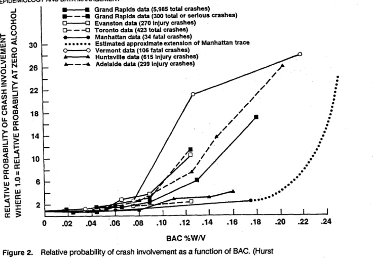
The relative probability of being involved in a crash is defined as the ratio of the BACs of comparison drivers to those of drivers involved in crashes. This probability remains roughly equivalent for crash-involved drivers compared with noncrash drivers up to about 0.08 BAC (figure 2). (However, these relative risk curves understate the risk of involvement at low BACs.) Although the rate of increased risk varies across studies (m part because some studies examine all crashes and some examine only fatal crashes), the. risk increases after about 0.08 BAC in all cases and increases dramatically after 0.10 BAC in most studies.

The curves depicted in figure 2 are based on groups of drivers of different ages who have varying experience with alcohol and with driving. Because of the heterogeneity of control groups and the lack of perfect comparability, the effect of alcohol at low BACs is masked by other variables. For example, the major shortcoming of the Grand Rapids study (among the most cited case-control studies) is the lack of comparability between the drivers involved in crashes and the control drivers regarding the frequency of consuming alcohol. This lack of comparability is the source of the apparent improvement in crash risk at low BACs in the Grand Rapids data (the much debated “Grand Rapids

(11)

45

Grand Raplds data (5,965 total crashes)

Grand Raplds data (300 total or serlous crashes) Evanston data (270 Injury crashes)

Toronto data (423 total crashes) Manhattan data (34 fatal crashes)

Estimated approxlmate extenslon of Manhattan trace Vermont data (106 fatal crashes)

Huntsville data (615 Injury crashes) Adelaide data (299 Injury crashes)

: : : : : : : : : : : -0 0 .02 .04 106 .06 .lO .12 .14 .16 .18 .20 .22 .24 BAC %WN

Figure 2. Relative probability of crash involvement as a function of BAC. (Hurst

1985.) Reprinted with permission.

dip”) and the understatement of the risk of crash involvement at low BACs. Hurst (1973) noted that the control group had a higher percentage of drivers who were regular consumers of alcohol. Their apparently greater tolerance for alcohol had made them safer drivers at low BACS than the drivers involved in crashes at low BACs, presumably because the latter had less experience as drinkers. Hurst recalculated the relative risk of crash involvement in the Grand Rapids data based on the drivers’ self-reported frequency of alcohol consumption (figure 3). He drew three conclusions from the results. First, drivers with frequent experience as drinkers are less likely to be involved in crashes than light and medium drinkers at comparable BACs. Second, regardless of the tolerance for alcohol, the risk of crash involvement increases with BAC. Third, the curves greatly underestimate the risk for the average driver at any BAC; they only demonstrate the relative hazard to drivers who regularly drink and drive. The curvilinear relationship between relative risk of crash involvement and BAC is therefore caused in part by the comparison of drivers with varying degrees of experience as drinkers and experience driving under the influence of alcohol. When experience with alcohol is controlled for, the risk of crash involvement increases with BAC without evidence of a threshold effect. As noted by Perrme (197%) in his review of the literature, the relative risk of involvement is not the same as evidence of causality. Given the many interacting factors that may contribute ‘to a crash (and the lack of data on many of them), the role of atry single factor is difficult to isolate. Three of the case-control studies deserve special attention because they also estimate the effect of alcohol on the probability of being responsible for a crash.

The methodology for estimating crash responsibility was first developed by McCarroU and Haddon (1%~) in their case-control study of fatal crashes in Manhattan. They

(12)

6ACKGFIOUND PAPERS

SELF-REPORTED DRINKING FREQUENCY . . . ..a. YEiRLY OR LESS .-’

-0- MONTHLY -= . 6.0 i - - W E E K L Y --- B X N V E E K 4.0 - DAILY I 1 I I I I 0 .02 34 .06 .08 BAC, %W/V

Figure 3. Relative probability of crash involvement by self-reported drinking frequency (Hurst 1973). Reprinted with permission from theJoorna/ofSafetyResearch, a joint publication with the National Safety Council and Pergamon Press, Ltd.

categorized the crashes into five classes, the first three of which were assigned responsibility:

1. Only one vehicle involved

2. Two vehicles involved but only one moving

3. More than one vehicle involved and in motion, with responsibiity assigned based on circumstances of the crash (cases in which there was any doubt were excluded from this category).

The Manhattan study is based on a sample of 43 drivers fatally injured in crashes that occurred between June i950 and June 1960. For the 26 drivers in the assigned responsibility classes, 19 (65 percent) had positive BACs, of which 14 (46 percent) had BACs greater than 0.10 . Of these 14 drivers, 12 had BACs of 0.25 or greater. Of 156 drivers randomly selected as controls at or near the sites of the crashes, 39 (25 percent) had positive BACs, of which only 8 (5 percent) were at or above 0.10 .

The Grand Rapids investigation involved by far the largest sample of all the case-control studies (5,985 crashes of all types) (Borkenstein et al. 1964,1974). By comparison, the 423 cases in the Toronto study constituted the next largest sample (Lucas et al. 1955; Hurst 1985). Using McCarroll and Haddon’s method for assigning responsibility, Borkenstein, Crowther, Shumate, Zill,

and Zylman

estimated

that 3,305

of the involved

drivers were responsible for the crash that occurred. They used the innocent drivers as controls.

The Vermont study was the third to estimate crash responsibility, based on 106 cases (all fatal crashes) (Per&e et al. 1971). These crashes resulted in 113 fatalities, and 97 of the drivers were assigned responsibility, again relying on the method developed by McCarroll and Haddon. Of the drivers judged responsible, 60 percent had positive BACs and 46 percent had BACs at or above 0.10. Perrine, Waller, and Harris (1971) also calculated a crash-responsible curve, but in contrast to the Grand Rapids study, the drivers stopped at roadblocks were used as controls.

(13)

EPlDEtdlCL~Y AND DATA MANAGEMENT

U ‘GRAND RAPIDS DATA. 3305 CRASHES. DRIVER ASSUMED RESPONSIBLE - MANHAlT’AN DATA, 24 FATAL CRASHES,

DRIVER ASSUMED RESPONSIBLE o----Q VERMONT DA-t-As 75 FATAL CRASHES.

DRIVER ASSUMED RESPONSIBLE

1

I I I I I I I I

.02 .04 .08 .08 .lO .12 .14 .18 .18 90

8AC % (WA’) OF DRIVER

Figure 4. Relative crash responsibility for drivers assumed responsible and those not assumed responsible as a function of BAC, where 1 .O = relative probability at zero alcohol. (Hurst 1973.) Reprinted with perniission from theJourna/ofSafefyReseafch, a joint publication with the National Safety Council and Pergamon Press, Ltd.

Hurst (1973) replotted the curves from these three studies on a logarithmic scale to facilitate comparison (figure 4). Although risk of crash responsibility increases as BAC increases in all three studies, several disadvantages with the underlying data should be noted.

The trend in the Manhattan data is based on a very small number of crashes: 25 responsible drivers with positive BACs. In addition, the trend at the higher BACs is greatly understated. For the fatal crashes in which the driver had a BAC of 0.25 or higher (about half those in the driver-responsible category), no driver in the control group had

an equivalent BAC. “Hence, the relative hazard calculated from the case/control ratio would be infinite within the range, were it possible to graph it” (Hurst 1973).

One of the shortcomings of the relative risk curve estimated in the Grand Rapids study is the inclusion of drivers involved in single-vehicle crashes in the group of responsible drivers. Although the responsibility of the driver is not in question, because of the nature of the crash, a control driver is not available. The published data do not provide sufficient detail to allow the curve to be compIeteIy recalculated without the single-vehicle crashes to determine the effect of including these crashes, but the available data suggest that the curve would shii to the right. It would still accelerate after 0.04 BAC and at an exponential rate, but the curve would not rise as quickly as shown in figure 4.

(14)

One problem with the Vermont data is the small number of crashes in the sample. In the comparison of crash risk as BAC rises, one. or two drivers are responsible in some of the BAC ranges. Chance occurrence could distort the results when-so few drivers are _/ the basis of the calculations.

Despite the weaknesses in the case-control studies, some important conclusions can be drawn. In several of the case-control studies done in the United States and abroad, a consistent increase in risk of crash involvement has been shoti. When experience with drinking is controlled for, this risk increases with BAC without any evidence of a threshold effect (or dip). The three studies that attempted to estimate crash responsibility showed that the risk of causing a crash increases even more rapidly than the risk of crash involvement as BAC increases (NRC 1987).

Another important aspect of the alcohol contribution to crash risk is reported by Voas (NHTSA 1985). To emphasize the signilicance of the difference in BAC between drivers assumed to be responsible versus those assumed not to be responsible for crashes, Hurst (1974) also presented an additional calculation on the data from the Grand Rapids study. His results for the drivers assumed to be responsible are represented by the center plot’ in figure 4. However, the probability of being innocently involved in a crash remains essentially level and does not increase with increasing BAC, the plot is basically flat and would lie between the relative crash probability of 1 and 2 in figure 4. The same result was found in the Huntsville/San Diego study by Farris, Malone, and Lilliefors (1977). These results provide further evidence for the causal role of alcohol in crashes. Other Roadside Research

The success and utility of the case-control procedures for investigating alcohol crash risk stimulated interest in using the roadside survey technique for evaluating alcohol safety programs by measuring the change in the number of high-BAC drivers actually on the roads. Standardized procedures for conducting roadside surveys were developed (Perrine 1971) and applied successfully in 28 of the 35 Alcohol Safety Action Projects (ASAPs) funded by the bepartment of Transportation between 1970 and 1975 (Voas 1972; Carr et al. 1974). In these programs, the roadside surveys were used to evaluate project effectiveness (Levy et al. 1978) by serving as a means to collect data used as the primary criterion or dependent variable (BAC). Roadside surveys were conducted before and after program implementation to measure the change in average driver BAC (ii any) resulting from project activities (Lehman et al. 1975). When used for program evaluation, sampling was conducted during periods when a high percentage of drinking drivers was on the road (i.e., Friday and Saturday nights) rather than at times and places at which accidents had occurred. By a return to the same sites, changes over time can be measured.

Roadside surveys provide a more direct method of evaluating alcohol safety countermeasure programs than does the use of accident data, because highway crashes result from a large number of factors (weather, roadway construction, economic conditions, etc.) that are unrelated to the evaluation of enforcement activities. The BAC values of drivers serve as an intermediate measure between action programs and the ultimate criterion of accident prevention. While a reduction in the average BAC of drivers on the road does not guarantee a reduction in crashes, the relationship between driver BAC and risk of crash involvement is close enough to make this measure a credible criterion for program effectiveness.

During the ASAP period (1970 through 1974), some 77 roadside breath-testing surveys of nighttime drivers were conducted. In addition, a national roadside breathtesting survey was conducted in 1973, and a computer archive of these 78 roadside surveys is stored at the University of Michigan Highway Safety Research Institute (Lehman et al. 1975). The tile contains breath-testing results, demographic data, and so forth, for some 78,000 randomly selected drivers, as well as 2,700 passengers. Analysis

(15)

EPIDEMIOLOGY AND DATA MANAGEMENT 49

of these aggregated data show the following percentages of drivers with BACs at or exwe&mg 0.10: 1 percent of weekday-early drivers, 3 percent of weekend-early drivers, and 6 percent of weekend-late and weekday-late drivers. Significant reductions in the percentages of drivers above the legal limit (0.10 BAC) were demonstrated for those jurisdictions that used this evaluation method (Levy et al. 1978).

Based on the utility of this roadside BAC measure in the ASAP program, it was

applied

again in a 4-year study of a special DUI enforcement effort in Stockton, California (Voas and Hause 1987). In this study, survey procedures were modified to permit low cost and low profrle surveys that were conducted every weekend for 3 k years (Hause et al. 1982). Drivers with a BAC of 0.10 or greater on Friday and Saturday nights decreased from 88 per thousand before the Stockton project to 50 per thousand during the third year.

The roadside survey technique also permits (through an application of Bayes’ Theorem) estimation of the probability that a driver at a given BAC will be arrested by the police. This procedure was first applied by Beitel, Sharp, and Glauz (1975) to the ASAP survey data in Kansas City. Hause, Voas, and Chavez (1982) used the same procedure in Stockton. These studies provided roughly similar results indicating that the chances of being arrested at a BAC of 0.15 is roughly 1 in 100, while the chance of arrest at 0.10 BAC is half that amount, about 1 in 200. Since both these studies involved intensive enforcement programs, they provide a reasonable indication of the maximum arrest rate that can be achieved with traditional patrol methods.

The ASAP experience with roadside research surveys and with the success of the manual for conducting and evaluating them (Perrine 1971) provided the basis for subsequent international activity. An invitational international workshop was conducted in Paris in an attempt to coordinate the methodology for roadside research surveys to be implemented in other countries in order to maximize the comparability of the obtained data. The workshop resulted in a useful manual (Carr et al. 1974) and comple- mented parallel activities being conducted under the auspices of the Organization of Economic and Cooperative Development. As a result of these activities, use of roadside surveys for international comparisons of countermeasure programs was stimulated in Canada, the Netherlands, Norway, Sweden, and Finland. The resulting data permitted an international comparison of driver BACs (Voas 1982), which indicated that

ap-

proximately 12 percent of drivers on weekend nights were at or above 0.05 BAC in Canada, the Netherlands, and the United States, whereas less than 2 percent of drivers were at this level in Scandinavian countries.

Although use of roadside research surveys has diminished in the United States since the end of the ASAP activities in the mid-197Os, the technique continues to be used effectively in other nations, for example, Canada, Australia, Denmark, and Norway. Nevertheless, a few studies of the population-at-risk in the United States either have been conducted recently or are currently being conducted. In the spring of 1986, U.S. National Roadside Breathtesting Survey II (Wolfe 1986) was conducted in a representative sample of 32 localities, 18 of which had

participated

in

the 1973 U.S. National Roadside Breathtesting Survey I (Wolfe 1974). Statistically significant reductions were found in the percentage of medium and high BAC drivers sampled at high-risk times

(Friday

and Saturday

nights from 10

p.m. to

3

a.m.). Drivers at or above

the illegal

BAC of 0.10 decreased from 5.0 percent in 1973 to 3.1 percent in 1986, drivers at or above a BAC of 0.05 decreased from 13.5 percent in 1973 to 8.3 percent in 1986. It should be noted that the breathtest completion rates were 86 percent in 1973 and 92 percent in l986.

In

Vermont,

a large-scale roadside research study involving a projected 42,000 nocturnal drivers sampled at high-risk times (Friday and Saturday nights from 10 p.m. to 3 a.m.) is currently being conducted. It is funded by the National Institute on Alcohol Abuse and Alcoholism (NIAAA, Grant AAO7876). This 5-year field study is primarily

(16)

designed to determine the prevalence of drivers with high alcohol tolerance, and to determine their salient and differentiating characteristics. Since the high alcohol tolerant driver is apparently rare, a large number of motorists (42,ooO) driving at high-risk times must be stopped and screened for BAC to identity a sufficient number of such people (40 to 60) to be able to conduct a meaningful study. In the process of conducting this field study, a large number of people will be breathtested using both the new passive alcohol sensor and the more traditional hand-held evidentiary devices. Approximately 4,000 of these motorists, sampled across the full distribution of BACs, will participate in extensive.personal interviews concerning self-reported background data; drinking, driving, drinking-and~driving, drugs-and-driving information and attitudes; and selected personality characteristics. Data will also be gathered on these motorists’ driver records, performance on the most valid field sobriety tests (gaze nystagmus, walk-and-turn, and standing steadiness), and ratings on clinical signs of intoxication. With a test completion rate of % percent, the results from the first 650 drivers indicate that 3.7 percent had a BAC of 0.10 or higher, whereas 10.2 percent had a BAC of 0.05 or higher. Although the sample size isstill relatively small, these 1988 data show a decrease in distribution of BAC when compared with data obtained in a 1974Vermont study (Perrine 1976) of 1,663 drivers at high-risk nocturnal times (Thursday, Friday, and Saturday nights between 1030 p.m. and 3 a.m.): 4.6 percent had a BAC of 0.10 or higher and 14.7 percent had a BAC of 0.05 or higher. Thus, these roadside studies of the high-risk population would seem to show that some progress is being made in the war on drunk driving, if motorists with BACs in excess of the legal standard (0.10) are taken as the criterion.

Enforcement Checkpoints

Police officers conduct sobriety checkpoints at which they stop motorists at random and test them for breath alcohol. Such activities are conducted primarily for enforcement purposes, although they also serve as general deterrence. Although useful data for epidemiologic purposes are available from these enforcement checkpoints, few sys- tematic studies have been conducted to analyze such data. If they were analyzed carefully and properly, these data could provide a valuable source of relatively low-cost information concerning the population-at-risk. In a recent Charlottesville, Virginia study, Voas, Rhodenizer, and Lynn (1985) evaluated the effectiveness of such sobriety checkpoints, especially in comparison with the drivers arrested for DUI by traditional roving patrols. In addition, thii study found evidence of police biases in those arrested, whereby both young drivers and women were underrepresented among arrested drivers, while minority and very high BAC drivers were overrepresented. Thus, such studies clearly demonstrate that researchers can avail themselves of enforcement checkpoints as an opportunity to collect valuable data for epidemiologic purposes.

Characteristics of Drunk Drivers

During the past 20 years, numerous statistical and clinical studies have been published on various aspects of the drinking driving problem. However, surprisingly little rigorous research has been published on characteristics of convicted DUI offenders, particularly when contrasted with the vast literature on problem drinkers/alcoholics, and on characteristics of drivers involved in fatal accidents. As suggested by Zylman (1974) and by Moskowitz, Walker, and Gomberg (1979), the population arrested and convicted of DUI offenses is not typical of impaired drivers in general or of drivers involved in alcohol-related accidents. The mean BAC of convicted DUI offenders in California during 1984 was 0.18-a concentration far in excess of the State’s 0.10 limit per se, and well beyond the level at which impairment occurs. In one of the few formal statistical studies of differences between alcohol-involved fatal accident drivers and convicted DUI offenders, Fridlund and Hagen (1977) used discriminant function analysis in comparing 146 DUI offenders in Los Angeles County with a sample of 191 alcohol fatalities. The DUI conviction group had significantly more prior DUIs, more prior reckless-driving

(17)

EPIDEMIOLOGY AND DATA MANAGEMENT 51 convictions, and more prior moving t&tic convictions. The differences on the incidence

of DUIs and reckless convictions was large, with the DUI group having about three times as many entries during the prior 3-year period.

Moskowitz, Walker, and Gomberg (1979) conducted a detailed review of the literature on DUI offender characteristics. This subsection relies heavily on their monograph for the pre-1979 literature, but concentrates on recent studies and studies not included in the 1979 review for its primary source references. However, a few pre-1979 studies of special importance are reviewed here as primary references even though they are also included in Moskowitx et al. (1979);

Moskowitz, Walker, and Gomberg organized their review by type of offender characteristic (prior driver record, age, etc.), and reached the following conclusions with respect to each domain:

l Marital status: DUI con&tees are much more likely to be divorced, separated,

or widowed than are non-DUI control populations. Some studies have reported five- to sixfold differences in rates compared with control populations.

l Employment history: Convicted DUI offenders are more likely to be un-

employed, with rate differentials ranging from two- to fourfold higher across various studies.

l Occupation: Convicted DUI offenders are more likely to have lower status

occupations. DUI offenders in blue collar jobs averaged 65 percent across studies compared with-5l percent for control samples.

l Income: Convicted DUI offenders tend to have lower incomes- about 18

percent lower than controls across the reviewed studies.

l BAC: The mean BACs for the offenders averaged from 0.18 to 0.28. (Statewide

California figures have consistently averaged 0.18.)

l Drinking behavior: DUI offenders drink more often and consume more alcohol

per sitting than do non-DUI populations. Beer is the preferred beverage of DUI offenders. The findings of the Southern California study by Pollack (1%9) are typical. Pollack reported that 18 percent of DUI drivers drank every day compared with 11.5 percent for a control sample. In terms of drinks per sitting, 35.2 percent of the DUI sample typically consumed five or more drinks compared with 5.7 percent of the control sample.

l Reason for drinking: Convicted DUIs (and alcoholics) are more likely to drink

to release tension and to cope with stress.

l Problems caused by drinking: Convicted DUIs are much more likely than

controls to exhibit poor health, family disorganization, financial problems, and poor job performance.

l Prior alcohol treatment history: Convicted DUIs are more likely than controls

to have previously entered some form of alcohol treatment program. The median across 20 studies was 6.0 percent, with a maximum of 42.5 percent. (Thii characteristic is highly dependent on the institution and delivery systems of a particular region, and would be expected to vary across jurisdictions and over time.)

l Problem drinking status: Studies using the Michigan Alcoholism Screening Test

(MAST) indicate that 54-74 percent of convicted DUIs fall in the pioblem- drinking and alcoholic range. Studies using the Mortimer-Filkins test produce slightly lower prevalence figures.

l Driving after drinking: Convicted DUIs are much more likely than controls to

drive after drinking. Pollack (1%9), for example, reported that 49 percent of DUI offenders admitted to driving at least once a week after two drinks compared with 12 percent of a control sample.

(18)

l Total prior- arrests: Convicted DUI offenders are more likely to have prior

arrests for both alcohol and nonalcohol offenses.

l Driving history: Convicted DUI offenders have substantially more driving

record entries of all types than do controls (more DUIs, more alcohol and total accidents, more moving traffic violations, and more license actions). The rate increases across studies and variables range from 100 percent to 500 percent. The driving record histories of convickd DUIs are also substantially worse those of medically diagbosed alcoholics.

l Personality traits: Convicted DUIs have a significantly higher prevalence of

personality trait disorders. They are more ‘likely than controls to exhibit neuroticism, depression, paranoid ideation, low self-esteem, and to have a lower sense of personal responsibility and control and greater. feelings of aggres- sion/hostility.

l Stress: Convicted DUI offenders are more likely to report experiencing stress

from family, financial, and job problems. .I

l Education: Convicted DUI offenders are more likely to be high school dropouts

and have fewer years of education. \

l Age: Convicted DUI offenders tend to be slightly older than non-DUI controls,

with the highest disproportionate concentration in age interval 304.

a Race: Most convicted DUI offenders are white, but minority groups (hispanics and blacks) are overrepresented compared with their representation in the population.

l Sex (not covered by Moskowitz): The great majority of convicted DUI offenders

are male. The range for females is from 5 to 20 percent, depending on the characteristics of the specific DUI population (first versus repeat offenders), region, and so forth. A large statewide sampling in California indicates that 13 percent of those convicted for a DUI offense in 1982 were female (Tashima and Peck 1986). Among fust and second offenders, females accounted for 17 percent and 10 percent, respectively.

Drinking Status

It is clear from the above summary that persons convicted of drunk driving offenses deviate greatly from the general driving population on a wide variety of characteristics. That DUI offenders contain a disproportionate number of problem drinkers would be expected, of course, since the offense of drunk driving is, per se, a problem associated with the consumption of alcohol.

The number of drinks required to produce manifestly detectable impairment in driving and the BACs typically attained by DUI offenders implies a level of alcohol consumption that is statistically deviant. Given the very low probability that any given incident of impaired driving will result in detection (arrest or accident), the percentage of DUI offenders who were simply unlucky, in the sense of getting caught in a rare instance of impaired driving, would be relatively small. One would therefore expect most

DUI offenders

to be heavy

consumers

of alcohol.

Most of the empirical literature, and most authorities in the area, agree with this conclusion, although controversy has developed over the percentage of DUI offenders who are alcoholics in the clinical disease context. This controversy stems more from semantic and epistemological complexities than from disagreements over data, and is not pursued here.

Lest the impression be created that opinion and data are unanimous on the drinking status of DUI offenders, the results of a recent California study of first offenders will be summarized in detail. This study was carried out by the Pacific Institute for Research

(19)

and Evaluation (PIRE); it was commissioned by the State of California pursuant to Assembly Bill 3405 (Stewart et al. 1987).

The major objective of ,the PIRE study was to develop a model curriculum and rehabilitation program for use by courts in sentencing fmt-offender DUI cases. HOW- ever, this review will only consider that component of the study pertaining to offender

characteristics (natural variation component).

Detailed biographical, drinking habit, and arrest-incident information &as collected by questionnaire on 5,052 respondents from 26 frst-offender treatment programs throughout California. The authors reported the following statistics from an analysis Of

the questionnaire responses:

l Median number of drii on day of arrest: 6 l Median BAC upon arrest: 0.16

l Median number of days in past year with four or more drinks: 60

0 Median number of days in past year with eight or more drii 4

l Percentage who did not feel intoxicated upon arrest: 35 percent

0 Median number of previous days in past year driven while impaired: 1 0 Percentage with prior DUI arrests: 20 percent

The authors categorized the drinking pattern responses into two typologies for comparison with a statewide general population survey. The more complex of the typologics was a ir-point continuum: abstainers, infrequent drinkers, light monthly, light

weekly, moderate weekly, and frequent heavy. Using a probit analysis to adjust for p~~pulation differences, the authors found no significant differences between the drmk-

ing frequency of the two groups after abstainers were removed from the general population sample.

The difference was significant, however, in the frequency of heavy drinking (five or more drinks at least once a week), with substantially more of the DUI offenders falling

into that

category. Nevertheless, fewer than 30 percent of the first offenders were placed in

this

category. In commenting on these findings, the authors concluded:

While defining a “typical pattern of drinking for all subjects is difficult, the median frequencies of use conditional upon the level of use at arrest is revealing: 40 percent of the subjects reported having had 8 or more drii on the day of their arrest. The median frequency of use at this level among these subjects was 14 occasions over the previous year and only one occasion in the preceding 30 days. A pattern of use including drinking 8 or more drinks at least weekly over the previous year was reported by only 20 percent of these subjects. Thus, for the majority of subjects, drinking at the level of use at which they were arrested is relatively infrequent (pp. 27-28)

. . . first offenders are not unlike the general population of drinkers in California in terms of the typical frequency of use. However, it appears that the incidence of heavier drinking is greater among first offenders (p. 32)

Thc authors also included a measure of alcohol dependency in their study. Subjects c‘n”‘@-tcd a Z-item

Alcohol

Dependency Scale (Skinner and Allen 1982), and the

‘c0rcS werc compared with those of clinically diagnosed alcoholics. Ninty-two percent ‘If ‘hc subjects pioduced scores “~&&~g a low level of alcohol dependency.” The aUt hors went on to conclude “the dramatic differences in these distributions suggest that d’pcndcnCT symptoms among first offenders are quite low, as compared to alcohol

‘rcJlmcnt

groups;)

Thc resu*& and conclusions of the PIRE study are at odds with prevailing opinion id most Prior studies in this area. If the findings are accepted at face value, the great

(20)

majority of first offenders fall within the bounds of social drinking Even the percentage characterized as heavy does not seem extreme. \ ₁

There are several ‘possible explanations. Fist, the PIRE study was limited to first offenders, and it is known that the percentage of problem drinkers among first offenders is lower than among repeat offenders.

Second, problem drinkers and DUI offenders are known to understate their drinking, sometimes dramatically. Stewart, Epstein, Greenewald, Laurence, and Roth (1987) acknowledge this possibility and recommend caution in interpreting the study f&lings. Although previous studies are also subject to reporting biases, many have included clinician interviews, psychometric instruments employing lie scales, and a variety of public agency data. No evidence is presented in the PIRE study to indicate that procedural controls were used to minimize the tendency of people to “fake good” or employ various forms of self-denial.

.s

Third, the first-offender survey only involved offenders who were sentenced to an alcohol program and who agreed to cooperate by completing the questionnaire. In California, 23 percent of first offenders are not assigned to programs. Approximately I.5 percent of the sample did not return a questionnaire.

There are also inconsistencies in some of the values derived from the self-report. For example, it would have taken more than a median of six drinks to produce a median BAC 0.16. The fact that 35 percent of the subjects did not feel intoxicated when arrested and that only 14 percent acknowledged being definitely intoxicated is cause for further suspicion.

Finally, it is difficult to accept the median estimate of only one incident of driving while impaired in the previous 12 months. The suggestion is that many of the subjects were not being candid in their responses.

The PIRE report also contains a description of first offender biographical and socioeconomic characteristics. The statistics of interest are summarized below:

l Male: 81 percent l Single: 46 percent

l Divorced, widowed, or separated: 21 percent l White: 68 percent

l Hispanic: 22 percent l Black: 3 percent

l High school dropouts: 22 percent l Median age: 30

l Unemployed or employed part-time: 30 percent l Median income: $16,500

These demographic characteristics are reasonably consistent with the portrayal from the Moskowitz review, particularly when allowance is made for differences in time and region. The percentages for ethnic minorities are somewhat lower than would be expected based on California ethnicity composition and prior evidence showing that some minorities (e.g., Hispanics) are overrepresented in DUI populations. It is important to recognize that the PIRE sample is limited to offenders entering first-offender programs and, within this subset, to those who returned the questionnaire. These factors could alter the representativeness of the sample.

Prior Driving Record

(21)

EPIDEMIOLOGY AND DATA MANAGEMENT 55 DUI arrest. Although one would expect overinvolvement in previous alcohol-related

accidents and convictions, the extent of DUI offender overinvolvement in nonalcohol related incidents is not widely recognized.

Statewide, data from Tashima and Peck (1986) indicate the following pretreatment w-month rates for representative statewide samples of 29,097fmt and7,797repeat DUI offenders:

Mean non-DUI Mean total Mean non-DUI related accidents accidents convictions

First offenders .17 36 13

Second offenders .1g .45 1.4

The above rates are more than twice the rates expected fora similarly stratified (age and sex) population of non-DUI drivers.

The Tashima and Peck (19&i) study and numerous previous California studies indicate that nonsuspended DUI offenders also accumulate worse non-DUI driving records (total accidents, total moving violations, etc.),jXlowing conviction for a first or repeat DUI offense (Sadler and Perrine 1984; Hagen et al. 1978; Hagen 19T7, Arstein- Kerslake and Peck 19235).

The most detailed analysis was performed by Arstein-Kerslake and Peck, who compared the subsequent 4-year driving records of first and repeat DUI offenders from Sacramento County with a general population group that was similarly age-sex stratified. The first and repeat offenders were grouped into quartiles based on their actual and predicted DUI recidivism. Except for the first quartiles (i.e., lowest 25 percent in terms of recidivism expectancy), all quartiles had substantially worse accident and traffic conviction records. The differences were also highly significant when summed across quartiles.

The above relationship between DUI offenses and driving behavior in general has been addressed by a number of other investigators (Maisto et al. 1979; Raymond 1971; Denberg 1974). Donelson, Beimess, and Mayhew (1985) consider the issue from the impaired problem-driver paradigm addressed in Simpson’s (1977) paper. This heuristic paradigm views the convicted DUI population as containing drivers whose drinking is subordinate to a larger problem of high-risk negligent driving. The alcohol impairment can combine, additively or synergistically, with negligent driving to increase risk, but the underlying problem-driving behavior exists independent of alcohol.

Although Donelsou, Beirness, and Mayhew stress the hypothetical nature of this paradigm, the premise that impaired drivers who drive aggressively and unlawfully are more likely to be apprehended is in no way hypothetical. It has also been established that DUI offenders with a prior history of moving violations represent substantially greater accident risks than DUI offenders with clean records (Sadler and Perrine 1984; McConnell and Hagen 1980; Peck and Kuan 1983).

The linkage

between

problem

driving and DUI offenses

is the very essence

of a recent

study by Donovan, Umlauf, and Salzberg (ii press). These investigators followed the driving records of 254 non-DUI-involved problem drivers over a 3-year period subsequent to initial ‘identification. Approximately 11 percent of the sample had a DUI conviction during that period-a rate live times greater than that of the general male driving population in Washington State. The study was replicated on a sample of 38,695 driver record fdes. The authors found that drivers with four or more moving violations were greatly overinvolved in subsequent DUI offenses, with 16.9 percent receiving an initial DUI conviction during a 3-year followup period. The DUI rate was particularly Pronounced for males under age 30.

(22)

DUI Recidivism

How do frost offenders compare to repeat offenders on the various characteristics described above? This question is, of course, related to the question of recidivism correlates and is best addressed by longitudinal recidivism studies.

The actual rate of recidivism cannot be dete.rmined in any general sense because it is inextricably tied to the length of the followup period, the length of record retention in a given State, the DUI arrest rate of a particular region or State, regional plea reduction practices, and the effectiveness of DUI countermeasures. In California, approximately 35 percent of all DUI convictions each year involve ‘drivers with prior DUIs within the preceding 5 years.

Recidivism prediction was directly addressed by Ellingstad (1974) as part of the evaluation of the South Dakota ASAP. Diicriminant analyses, performed separately for problem and nonproblem driers, assessed the predictabiityof a dichotomous DUI recidivism measure using 14 variables related to prior .wnviction history, demographic characteristics, drinkii pattern, and Mortimer-F&ins score. The problem-drinker group yielded the highest level of prediction. For the 1,744 problem-drinker clients, of whom only 12.6 percent were actual recidivists, prediction of subsequent Zyear DUI recidivism was significant at the 0.001 level. However, only 4.4 percent of the variance in recidivism was accounted for by the discriminant function (multiple R -0.209). Of the 14 variables used for the recidivism analysis, only 6 had a significant u&&ate relationship -with recidivism: prior DUI convictions, reckless convictions, total convictions, marital status, drinking pattern, and Mortimer-Filkins score. All relationships were in the expected direction - that is, less favorable values were associated with increased recidivism.

The level of recidivism prediction reported by Ellingstad (1974) was greater than that reported by Burch (1974) in her analysis of the Los Angeles ASAP. A multiple regression analysis was conducted for approximately 1,000 clients with the objective of predicting subsequent 7-month DUI recidivism using treatment, age, accident, and wnviction measures as predictor variables. The actual 7-month recidivism rate in the sample was approximately 1. percent. The analysis indicated that 2.4 percent of the variance in recidivism could be accounted for by the seven predictor variables (R = 0.155, p c 0.01). The relatively low level of prediction reported by Burch results at least in part from the brief 7-month period during which recidivism data were collected.

As part of the evaluation of the El Cajon Drinking Driver Countermeasure Program, Wendlmg and Kolodij (l!V7) collected data on driving history, criminal arrest record, probation officers’ evaluation of problem-drinking severity, and Mortimer-Filkins diag- nostic scores from 1,740 DUI offenders. These measures served as predictors of the yearly rate of recidivism (DUI and reckless-driving convictions). The duration of data collection subsequent to treatment ranged from 0 to 72 months. Stepwise multiple regressions were performed for each half of the sample, and then each equation was applied to the other half of the sample in order to provide a measure of cross-validation. Although Wendling and Kolodij report impressive Rs in the range of 0.40, the high levels of classification error upon cross-validation indicate that the construct multiple Rs were inflated.

Development of a prediction model to identify likely recidivists among a sample of Los Angeles DUI offenders was one of the main objectives of Pollack, Dideuko, McEachern, and Berger (1972). Three models were developed and evaluated: multiple regression, discriminant function, and empirical bayes. The authors reported a hi degree of classification accuracy for drivers with extremely high predicted recidivism expectancies. However, since these drivers represented only a small part of the total recidivist population, it could not be concluded that recidivism can be accurately predicted. On the contrary, the data indicated that the classification error would be substantial for drunk drivers with nonextreme recidivism expectancies. Although no