The Introduction of a Private Wealth Module in CAPP_DYN: an Overview

Materiali di discussione

Viale Jacopo Berengario 51 – 41100 MODENA (Italy) tel. 39-059.2056711Centralino) 39-059.2056942/3 fax. 39-059.2056947 Università degli Studi di Modena e Reggio Emilia

Dipartimento di Economia Politica

\\ 630 \\

The Introduction of a Private Wealth Module

in CAPP_DYN: an Overview

Carlo Mazzaferro

1

Marcello Morciano

2

Elena Pisano

3

Simone Tedeschi

4

June 2010

1

University of Bologna and CAPP

2

University of East Anglia, ISER and CAPP

3

University of Rome “La Sapienza”

4

1

The Introduction of a Private Wealth Module

in CAPP_DYN: an Overview

Carlo Mazzaferroa_{, Marcello Morciano}b_{, Elena Pisano}c_{, Simone Tedeschi}d

Abstract

We describe and discuss the integration in the dynamic micro simulation model CAPP_DYN of a new module in which household’s savings and asset allocation are modelled. In particular, our efforts are addressed at accounting for some possible behavioural change in household savings within a framework which remains mainly probabilistic. To this end, our strategy has been that of adopting the traditional stochastic micro simulation approach for assets allocation, while approximating a structural framework for estimating consumption/saving behaviour. Our framework has been inspired from a basic version of the life cycle hypothesis as formulated in Ando and Nicoletti Altimari (2004). In fact, we emphasize the role of life cycle economic resources in households consumption decisions, yet we further modify their empirical model in order to account for internal habit formation and subjective expectations on pension outcomes in the econometric stage. Moreover, among the several probabilistic processes we introduce in the simulation program and present in this paper, we conceive the modelling of intergenerational transfers of private wealth as an original contribution to the existing micro simulation literature.

JEL Classification: D31, D12, D91, C23, H55, J11

Keywords: Microsimulation, Household consumption, income and wealth distribution, intergenerational transfers, social security.

a _{University of Bologna and CAPP}

b_{University of East Anglia, ISER and CAPP} c

University of Rome “La Sapienza”

d

2

1. Introduction

In micro simulation literature a limited number of models are provided with a module aimed at analyzing and projecting the evolution of private wealth along time5_{. Indeed, introducing a wealth module in a dynamic micro} simulation model implies undoubtedly advantages, yet it entails some significant drawbacks. On the one hand, in fact, the modelling of wealth permits researchers to draw a more complete picture of disposable income dynamics (i.e. labour plus capital income components) and of households' well-being distribution, allowing also to analyze the future redistributive effects of reforms which are going to affect - as expected in Italy – both public and private pension pillars. On the other hand, however, it increases significantly the complexity of the model, explicitly arising the debated question of the choice between a mechanical and a behavioural approach.

The traditional one, called also ‘probabilistic’, assumes relations estimated (through reduced forms) on data to be structurally stable over a period of about 50 years. To our knowledge, existing models – especially population based - including a wealth module have mainly relied on an arithmetical-probabilistic approach, providing a deterministic representation of household decisions such as transmission, accumulation and decumulation of financial and real wealth, though enriched with several stochastic processes in order to account for heterogeneity and uncertainty in the dynamic simulation of all variables. In particular, some processes are modeled by means of reduced forms estimated on information from panel data surveys6 _{- or administrative panel datasets matched} with surveys7 _{- sufficiently long to estimate steady relations for the accumulation and spend-down of the main} private assets, with no explicit modeling of household consumption decisions8 _{and mainly focusing on first} round budgetary and distributional effects of possible policy change.

Differently, the ‘structural dynamic’ approach models economic variables as a solution of a utility maximization problem subject to constraints given by the institutional framework or policy, trying to represent second round (behavioural) effects, which could either strengthen or offset the first order impact of reforms depending on the nature of responses. In this second scheme, a value function characterised by uncertainty in one or more arguments is maximized, and the solution is derived by backward recursion under dynamic programming. Therefore, the researcher attempts to estimate the “deep” underlying preferences, which are assumed to be stable in the long run. However, in large-scale dynamic cross-sectional models the structural part (when does exist) does not involve all the simulated processes but, usually, integrates as an input, with many other probabilistic processes (see, for instance, Harris, Sabelhaus and Sevilla-Sanz, 2005).

5 _{PENSIM2 in Great Britain, MINT3 in the United States or SESIM III in Sweden are some of the most relevant examples.} 6 _{FRS and BHPS for Pensim2, PSID and SIPP for MINT3.}

7 _{LINDA, the main source for SESIM, is an administrative dataset starting from 1960 which covers about 3.5% of Swedish}

population.

8 _{Models based on surveys (PENSIM, MINT) estimate the unconditional probability for a household to hold a certain asset}

– and then the amount – at an age preceding retirement. Then they simulate the asset yearly evolution until household extinction .

In SESIM, wealth is represented by means of a two part model as well; however, accumulation dynamics is simulated also at younger ages. A special effort in SESIM has been addressed in modeling a specific dynamics for private pension wealth (pension funds), starting from a reconstruction of accumulated tax-deferred pension savings.

3

The reasons for this are manifold. First, dynamic micro simulation models do not explicitly allow for the supply side of the economy and therefore, at least so far, have not been tools for general equilibrium analyses (about linking CGE and Microsimulation models, see Peichl 2008). Second, a practical limitation with this approach is that the estimation of an entirely structural modelling of the processes usually involved in a dynamic population MSMs would imply an excessively heavy computational burden at the state of the computer technology.

Nevertheless, the introduction of some form of behavioral function is extremely important in models aimed at analyzing long run effects of radical reforms in the social protection system as long as these are expected to affect saving and labour supply decisions.

The present work aims at developing and integrating the dynamic micro simulation model CAPP_DYN9 _with a new module in which household’s savings and asset allocation are modelled. In particular, our efforts are addressed at accounting for some possible behavioural change in household savings within a framework which remains mainly probabilistic. To this end, our strategy has been that of adopting the traditional stochastic micro simulation approach for assets allocation (investments decisions), while approximating a structural framework for estimating consumption/saving behaviour.

On the one hand in fact, consistently with the nature of CAPP_DYN, the wealth accumulation and spend down module allows the representation of several processes characterized by a high degree of institutional details by means of a large set of empirical ‘ad hoc’ solutions. On the other hand, since saving behaviour can be strongly affected by radical reforms, as the ones adopted in Italy, the traditional probabilistic approach based on reduced-form estimations on current data would fail in representing long run relations, especially when rereduced-forms have not been fully phased-in yet, due to a long transitional phase. In such cases, in order to account for the change in expectations and to give a proper account of household saving/consumption decision, the empirical model needs to be "clasped" to a theoretical framework.

Our framework has been inspired from a basic version of the life cycle hypothesis as formulated in Ando and Nicoletti Altimari (2004) (AN henceforth) as most of their assumptions made in order to obtain a computable algebraic expression for the household consumption rule as well as several of their enlightening ‘heuristic’ solutions appeared reasonably compatible with the nature of our model. However, while AN aimed at carrying out a forecast for the evolution of aggregated saving, we are mainly interested in a long-run distributional analysis of income, consumption and wealth, especially in the individual’s retirement period.

In order to better represent behaviours and catch heterogeneity in a micro framework, we also allow for

internal habit formation, as this hypothesis results particularly helpful in reconciling the life-cycle theory with most of the empirical evidence on household inter-temporal decisions (See, among others, Meghir and Weber, 1996; Seckin, 2000; Angelini, 2009). This approach assumes individuals/households derive utility not only from current consumption but also from the comparison with a reference level of it, which, in a simplified version, is represented by previous period (lagged) consumption. As a result, this setting has the important implication that

4

agents attempt to smooth both level and variation in consumption. Therefore, as in the original AN microsimulation analysis, we emphasize the role of life cycle economic resources in households consumption/saving decision, yet we further modify their empirical model in order to account for habit persistence and subjective expectations on pension outcomes in the econometric stage; in addition, we allow for liquidity constraints on consumption expenditure in the simulation program.

In the next section we briefly outline the stylized functioning of the Wealth Module, by illustrating the sequencing of the main tasks i.e. transferring, investing, and allocating wealth among main assets. Then, in section 3, we describe the theoretical background for modelling the behaviour of households in distributing resources for consumption over the life cycle. In order to achieve this aim, we focus on the estimation of household lifetime human resources - and their specific components (section 3.1) - a key variable employed for the estimation of the consumption rule explained in section 4. In section 5 we discuss the empirical strategy for modelling intergenerational transfers and their mechanics in the simulation program. Data issues and other empirical details, as well as the some insights on income netting algorithms preceding the module itself, are provided in the Appendices.

2. The Wealth module sequence

The Wealth Module of CAPP_DYN starts the simulation from the panel dataset provided by the pre-existing blocks of the model, where demographic events, labour incomes and a full range of social security benefits are simulated for the period 2008-205010_{.Consistently with the previous part of the model, the base year population} is represented by the 2002 wave of the Bank of Italy’s Survey of Households Income and Wealth (SHIW). As the SHIW suffers of an heavy financial assets under-estimation due to under-reporting, we employ the adjusted wealth data from D’Aurizio et al. (2006) on the same source11

.

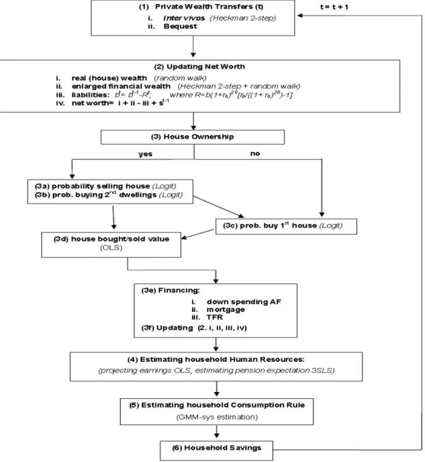
The sequence of processes for the mechanisms of formation, transmission and accumulation/spend down of household wealth are synthetically reported in figure 1.

The module adopts the traditional recursive logics of dynamics MSMs , included CAPP_DYN, – i.e. it estimates all the variables in year (t) and uses them to determine the transition probabilities in year (t+1). In addition, some of the simulated processes have a dynamic specification themselves and have been estimated on

10 _{The main implication is that feedbacks from wealth to demographic and occupational decision are not allowed for. In a}

further development of the research the Wealth Module will be sequentially integrated with the other pre-existing modules.

5

the panel component of SHIW using the lagged dependent12 _{among the covariates. The decisional unit for the} wealth processes is the household13_.

In short, the module begins by modeling the intergenerational transmission of wealth, which includes inter vivos

and mortis causa transfers. Following, the model updates each wealth component as a random walk, with its specific asset returns. Concerning financial wealth, before determining the current value, we preliminarily estimate the propensity and (if positive) the share of financial resources allocated in risky assets, using a selection model à la Heckman (results provided in the appendix B).

Next the module runs the investment part which is leaded by the house equity decisions (buying, selling and amount): these processes are carried out by means of a traditional two part model, combining discrete choice models (logit, plus Monte Carlo techniques in simulation) for the probability of being a seller or a buyer, and OLS models for the determination of the amount of the house bought. Every time a household is selected for a transition in the housing market, debt (i.e. stock of capital borrowed) and the new mortgage instalment (if any) are re-computed.

In case of a purchase decision, the model distinguishes among three modalities of financing the assets which will be described in details later in the section. The final steps of the loop determines yearly household consumption expenditure, provided the computation of the Human Lifetime Resources, and ultimately performs the last recursive process, i.e. the determination of yearly household savings. In figure 1 we show the structure of the Wealth Module and the sequence of its main tasks.

12 _{CAPP_DYN is a discrete-time annual model, while our main estimation dataset (the Bank of Italy Survey of Household Income} and Wealth) has a biannual frequency. This fact causes an underestimation of persistence in the simulated dynamic models. We are aware of this problem, nevertheless, at the state of the art, a annual panel data source with the information we need is not available for Italy and we believe the advantages of fitting, on the whole, a better model (especially for the consumption rule) overtake the drawback of an underestimated persistence.

13 _{Consistently with the demographic hypotheses which ground CAPP_DYN we use a definition of household which}

6

Figure 1: a stylized scheme of formation and transmission of wealth in the Wealth Module

For simulation purposes, we adopt a re-coding of SHIW wealth variables in two macro-aggregates: (a) house equity (real wealth) (b) an enlarged financial wealth component, which includes all financial assets plus tangible goods other than real estate (which will be assimilated to non-risky assets). Net worth is obtained by subtracting financial debt (if any) from total gross wealth.

As mentioned above, the first simulated events are the intergenerational transfers of wealth between parents and children outside the family of origin. The inter-vivos transfers have been modeled by means of a probabilistic approach based on a Heckman two steps procedure in order to account for the selection bias, while bequests have a mechanical connotation. It is worth noticing that, due to insufficient information on financial transfers in the SHIW for our purposes, a different micro data source specifically focused on this issue has been

7

employed: the Survey of Health, Ageing and Retirement in Europe (SHARE). Details on the econometrics and the functioning of such a crucial sub-module are discussed in section 5.

Once transfers have fully accomplished14_{, every household (included the new born ones), have an initial} wealth stock.15 _{Next, an updating of wealth stock is operated by assigning a specific return on each assets in} order to determine current wealth value. Returns are derived from an i.i.d draw from a specific normal (or Pearson) distribution with mean, variance (and kurtosis) derived from available time series for Italy (see footnotes 13, 14, 15 and 18)16_{. This step introduces the individual portfolio risk in private accumulation process.} The current house equity value of household h, (AHt_{) is obtained by multiplying the lagged value of real wealth} by (1 plus) the rate of return on real assets rht (random walk) 17. Concerning financial wealth, in order to account

for differential returns on the share of risky (߮t ₎18 _{and non-risky}19 _{assets, we preliminarily estimate financial} wealth allocation between these two components with a dynamic model20 _{accounting for persistence in risk} attitude21 _{and for the role of other observables (see appendix B). Since (in the baseline) we assume the non risky} share of financial accrues a null real return, the weighted rate of return on overall enlarged financial assets amounts to ߮t_rf t _{, where the latter rate is a specific return on financial risky assets obtained as an i.i.d draw from a}

asset-return-specific distribution22_{. The updated value for the enlarged financial aggregate for the household} (AFt_{) is then determined as the lagged financial wealth multiplied by (1 plus) the weighted returns and then} increased by the previous period savings (St-1_{). The outstanding debt is, in first stance, obtained by subtracting} the capital component of mortgage instalment paid in the previous period (Rt_{cap) from its lagged value (} t-1

B ). Here we adopt the convention that all households repay the mortgage in 20 years23 _{(i.e. roughly the average} mortgage duration in Italy, according to Rossi, 2008); thus, capital mortgage instalment Rt_{cap amounts to 1/20 of}

borrowed capital stock (Bt_{), while total installment (including interest) is computed} as t ₌ t_{(1+ )}20_ _{((1+ )}20_−1)

tot m m m

R B r r r , where rm is assumed to be normally distributed with mean equal to 3% and

standard deviation amounting to 0.5% (in the baseline). For this formula to be true, we assume the borrowing

14 _{See section 5 for a thorough description of the private transferring processes}

15 _{This stock, in the first year of simulation, is drawn from the base year population dataset (SHIW 2002) and it is}

stochastically processed by the transfer sub-module.

16 _{We consider different hypotheses on the returns of the various assets in order to carry out sensitivity analyses, obtaining a}

benchmark, a low and a high accumulation scenarios.

17 _{In the benchmark scenario we have adjusted the average return over the 1970-2007 period from Muzzicato et al. (2002)}

amounting to about 2.5% by imputing a lower (very long run) rate (2%). At the same time we impute a moderate 8% standard deviation, close to that estimated by Cannari et al. (2008) for houses prices in Italy.

18 _{This aggregate is composed of stocks, mutual funds, private bonds, foreign government bonds, shares of limited liability}

companies.

19 _{Non-risky assets include bank and postal deposits CDs, PCTs, BFPs and government securities. We also added real}

(tangible) goods other than real estate.

20 _{Such allocation is estimated through a Heckman two steps model.} 21 _{A static model determines initial conditions for new households.}

22 _{In the benchmark simulation we assume a 3% real returns with a standard deviation equal to 18% and an excess of}

kurtosis of 2.4 for risky assets. These values amount to a weighted average among short, medium and very long run returns for Italy computed by Dimson et al. (2006). Figures for a wide set of countries are available in the DMS Global Returns database.

23 _{If a household extinguishes before the debt has been repaid, it simply transmits its overall net worth to its heirs according}

8

rate – rm – to be fixed over time once the mortgage has been subscribed and the mortgage repayment to be

constant. The net wealth is then given by the sum of real and financial wealth minus the outstanding debt (i.e. mortgage being the only form of borrowing we allow in the model).

In the following step the model simulates choices affecting the stock of real estate and the number of dwellings owned by the family. The decisions of purchasing or selling a house work on a set of discrete choice model (logit, estimated on the pooling of 1989-2006 waves of SHIW-HA, see Appendix C) combined, in simulation, with Monte Carlo techniques and then the totals are calibrated to match an external source (ISTAT, 2005)24_{. First, the model distinguishes between households already owning at least a house, which are allowed to} sell a property, and households not owning any house equity, which are not allowed to sell. Once the family is selected for the “sale” event, the value of house equity sold AHst _{is “heuristically” assumed to be the current} value of real wealth divided by the number of houses owned. The new value of household real wealth is the difference between the current real wealth and the value of the sold house.

The financial wealth is assumed to increase by the value of equity in case exceeding the existing debt, while the latter (if exists) falls by the price of equity sold up to its outstanding value; finally, the new mortgage (total and capital) instalment is computed on the new debt (if any).

When a household is selected – through an analogous procedure (logit) – for buying, the value of the purchased dwelling is estimated by means of an OLS on a pooling of SHIW cross sections (1989-2006) using the ratio of house value to household net wealth as dependent variable. In case a household is selected for buying, the model distinguishes among three cases:

i) purchase with down-spending up to 90%25 _{of the enlarged financial wealth; in this case financial wealth} decumulates by the price of the house bought, real wealth increase by the same amount and the eventual debt does not vary;

ii) if the price of the house exceeds the 90% threshold, the financial advance can be complemented with creation of new debt for the difference between the value of the house and the 90% of financial wealth; real and financial wealth are updated accordingly;

iii) if at least one of the two spouses has an accrued end-of-service allowance26 _{and the purchase concerns} the first house, a 70% redemption of it is allowed as a set-off of debt contracted in ii), possible difference exceeding the debt re-integrating the financial wealth (decumulated by 90%).

24

Since SHIW data seems to severely under-report the official trade flows in the housing market for the household sector, we fit the econometric models in order to model systematic differences in house equity decisions according to some observable characteristics then we align the totals to match external aggregate data. According to ISTAT among 2002 and 2008 in Italy around 1 million of real estate buying and selling per year have been recorded. This level corresponds to about a 4.5 percent households per year involved in house equity purchasing/building. We assume this frequency to be stable all over the simulation.

25 _{This is an assumption aimed at avoiding households to completely run out of their overall resources.}

26 _{In Italy, private sector employees benefit of an additional relevant resource at retirement which is called TFR}

(end-of-service allowance). In practice, TFR is a deferred share of wage, which can also be partially redeemed in some special cases, and in particular for the purchase of the 1st _{house or can be completely or partially devolved to complementary pension}

9

Finally, since the issued debt may be excessively high due to low financial assets relative to the price of the house, we operate a control on the sustainability of mortgage by imposing a ceiling to the (total) instalment, as the 40% of the current household net labour and pension income27_{. In case the instalment exceeds the threshold,} we force the instalment to the ceiling and re-compute the maximum sustainable debt given current resources.

Subtracting the pre-existing debt from this amount, one gets the maximum amount which can be loaned in the current period for the purchase of the house. Finally, the maximum value of house bought consistent with the new stock of debt is re-computed by summing the 90% financial resources and the maximum amount which can be loaned for the current period, plus the 70% of TFR for households which are constrained despite its redemption.

In the last steps of the loop the model predicts household human lifetime resources, which are the present discounted value of labour incomes stream up to retirement plus the pension income flows up to household extinction (see section 3.1 for details). Such aggregate is crucial for determining household consumption expenditure28 _{and finally yearly household savings are obtained as the difference between disposable labour and} pension incomes (net of mortgage instalment) and consumption. In the following sections we try to focus, one by one, on the main aspects we briefly mentioned in this section.

3. The households saving/consumption behaviour

In this section we illustrate the theoretical background modelling behaviour of households in allocating resources for consumption among different periods of their life. Our main task is to fit our data as better as possible while, at the same time, representing household consumption behaviour through a quite general expression for the consumption rule. This latter, once estimated, is implemented in the simulation program and aims at catching some possible behavioural reactions related to gradual changes in pension outcome expectations as a consequence of a radical social security reform which is characterized by a long transitional phase.

Assuming a homothetic - non-separable over time - utility function29_{, a closed-form life-cycle consumption} function from the optimization problem as elaborated in Modigliani and Brumberg (1954 and 1979) can be derived. Hence, our general formulation - in order to get an approximate optimizing model - is given by:

It is computed as 6.91% of the yearly gross wage and can be reasonably approximated with one gross monthly wage. It accrues at an yearly rate equal to 1.5% plus 75% the inflation. The introduction of TFR in the model serves to a twofold purpose:

1) allows for financing house purchase, making liquidity constraint less bounding 2) modelling the financing of complementary pension funds.

At the moment we have attempted to model the first issue, although, the inclusion of TFR in the model paves the way for future developments of the second point whenever data availability will allow to model such an aspect.

27 _{The average incidence of mortgage repayment on household income is around 30% in Italy (Rossi, 2008)}

28 _{Actual consumption cannot exceed the sum of all disposable households income and the “liquid” financial wealth} [(1-߮t_{)AF] net of any mortgage installment. Of course for some household this constraint is bounding and they are not allowed}

to consume their “desired” amount of resources.

29 _{Nagatani (1972), Hayashi (1982) and Zeldes (1989) argue a sensible way to account for income uncertainty, without}

10 1 0 1 1 E U ( , ; ) s.t. (1 )[ ] 1 t i i t i t i t i t t a a a C i t t t a t t a a a a Max C C H A A r y C φ π + ∞ + + + − = − −     = + + − −

∑

Where:

a = age of household head

t a C = current consumption 1 t a

C − = last period consumption for the same household (internal habit)

t a

A = non-human household wealth in year t when the age of household head is a

t a

y = current household disposable income (earnings and pensions) in year t when the age of household head is a

ߨ= period constant probability of household extinction30

H = household characteristics and type

r = real interest rate

Following Willman (2003) we can derive an algebraic expression for current consumption which in its implicit form is given by:

(

1 1

)

1 ( ) = ; , , ; A , y , (r, , ) (1) t t t t t a a a a C H f C − a

π

H −₋ HR H a

Where, in particular, HR represents the (expected) life-time human resources (or human wealth) given by the discounted future labour and pension incomes stream. As we are going to explain in the next sub-sections the "structural" element of the equation resides in the introduction of expectations about future income stream, through the role of human resources, as a determinant of household consumption. This approach requires in turn HR to be re-programmed every period. Cat 1

−

represent the role of habit in consumption.

For the estimation we chose an empirical specification which nicely describes the consumption/saving behavior of Italian household in our sample, summarized by the following formula:

1 1 2 1= ( ) ( ) (2) t t t t t k k t t k C C f a A y D H HR ρHR β β β − + + + + +

∑

31 For our practical purposes we neglect uncertainty in the future income stream. Moreover, we assume the discount factor to be equal to the exogenous growth rate in productivity (wage growth) in every period.

30 _{Following Blanchard (1985) agents face each period a constant probability of death (π) - instead of being infinitely lived -}

implying uncertain lifetime. For practical needs of our dynamic micro simulation framework we neglect such a source of uncertainty in the estimation and in the simulation of the consumption rule, by assuming households take as reference for household life time planning the expected age of death of surviving spouse (Tt_{) as in Ando and Nicoletti Altimari (2004).}

11

We will discuss the implications of such an empirical specification and the econometric estimation in section 4.

In the dynamic simulation program this equation provides us with a predicted value for the current level of consumption Cˆt. In order to account for the role of liquidity constraints, which should not be neglected in a distributional analysis, we compute current simulated consumption as:

{

ˆ

}

min , y (1 ) (3)

t t t t t t

tot

C = C + −

ϕ

AF −R

i.e. current household consumption can never exceed the sum of current disposable income plus the liquid share of enlarged financial wealth (non risky assets), net of the mortgage instalment (if any).

3.1 Household lifetime human resources (HR)

Before turning to the proper empirical specification of the household consumption rule, we focus on the definition of total household expected Human Wealth, whose estimation is propedeutic to the estimation of the consumption rule. The expected value of Human Wealth (or human resources) is empirically obtained by aggregating spouses' individual projected (after tax) incomes (earnings and pensions), plus the stream of adult children's expected labour incomes up to the age of 30, plus one year of earnings contribution of active children over 30. That is the assumptions are under 30 active children will leave the family of origin at 30, while over 30 active children are going to exit in one year. We know these are arbitrary hypotheses that leave room for refinements on the base of an in-depth study of the evolution of individuals demographic behaviour. However, at the state of the art they represent sensible, though simplifying, hypotheses that, as we will show in section 4, provide a good fit of our data in the analysis of household consumption behaviour.

In algebraic terms:

(

)

(

)

(

)

30 2 , , , 1 1 1 1 1 0 if

( ,

, )=

+

1

1

1

j k k k k k j k k k t t t a p a T a p J j a i k a i k a i t i i t i k i i k i i j i p a

w

w

P

HR i H a

E

E

I

E

r

r

r

− − − − ₊ + + = = = = = = ≤































₊























+

+

+







_



_









∑ ∑

∑

∑ ∑

active

Spouses' human resources

(4 )





































children's projected resources up to 30 where: k = 1,2 adult members

j = active children up to 30 living in the household

+

, k

t k a i

w

= net labour income of household member k (or j) expected in year t when he/she will be aged a+i

31 _{As we discussed above our reference propensity to consume out of human resources is the two year lag value of the}

12

,

t k a i

P

₊ = net old age pension benefit of household member k expected in year t when he/she will be aged a+i, or, if already retired, projection of current old age (or survivor) pension benefit in year t when he/she will be aged a+i

pk = expected retirement age for spouse k

ak = age of spouse k

Tk = expected death age for spouse k (ISTAT projections)

Therefore, in order to evaluate this (stock) variable we need to evaluate its three main components, that is the household life time labour income, the expected social security wealth for active individuals and the current (residual) social security wealth for the individuals who are already retired. It is worth noting that in the simulation program the predicted values of estimated equations used to build HR are re-computed – using the current simulated values of explanatory variables - every year in order to obtain the current value of HR which, in turn, is a determinant of the yearly simulated consumption.

These topics will be the subject of the next two sections.

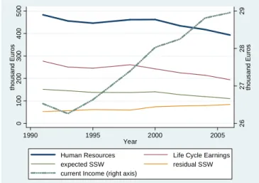
To conclude this sub-section we show the evolution of the variable HR and its components all over the estimation period and across the households population in SHIW data (figure 2).

From 1991 to 2006 the average value of the household human resources decreases from 482 to 393 thousand Euros while the average current household income (excluded capital incomes) increases from 26.5 to 28.9 thousand Euros (all values are in real terms, price 2002). This decreasing trend of HR is explained by the downward trend of the expected household life cycle earnings (from 277 to 194 thousand Euros) and the expected social security wealth (from 151 to 110) components and is partially offset by the increasing trend of the residual social security wealth component (from 52 to 84, representing the pension wealth of those individuals who are already receiving an old age or a survivor pension benefit).

Figure 2: Average evolution of HR and its component vs current income (1989-2006)

2 6 2 7 2 8 2 9 th o u s a n d E u ro s 0 1 0 0 2 0 0 3 0 0 4 0 0 5 0 0 th o u s a n d E u ro s 1990 1995 2000 2005 Year

Human Resources Life Cycle Earnings expected SSW residual SSW current Income (right axis)

13

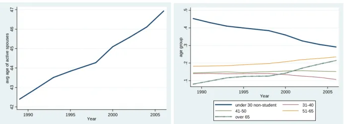
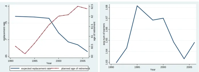
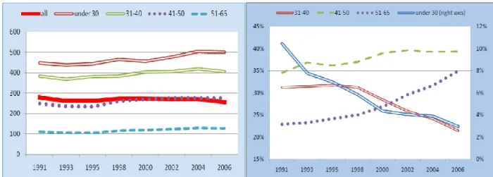
Demography plays a crucial role in the relative weight of each HR component. In figure 3 (left panel) we show the mean age of the active spouses (i.e. those who contribute the most to the life cycle earnings component of the family) which increases from 42.4 in 1989 to almost 47 in 2006. This fact implies, on average, a shorter residual active life also with respect to the planned age of retirement which, from 1993 to 2006 increases, on average, 2.1 years only, passing from 60.1 to 62.4 (figure 4, left panel). At the same time the average number of earners in the family (figure 4, right) just slightly increases, passing from 1.63 in 1991 to 1.65 in 2006 with its peak in 1995 (1.68 earners per household). With regard to the weight of different age group in the society, we can notice a steady downward trend of non-student under 30 (from 45% to 29%) mirrored by an as much steady upward trend in the weight of over 65 individuals (from 8% to 21.4%). This evidence explains the increase in the residual social security wealth component of HR.

Finally, with regard to the decreasing trend in the expected social security wealth component of HR, a non-negligible role is attributable to the significant fall in the average expected replacement rate32 _{which, especially} after 1998 decreases ten percentage points, from about .76 to about .66 (figure 4, left panel).

Figure 3.: Average evolution of active spouses age (left panel) and the weight of different age groups(right panel) (1989-2006)

4 2 4 3 4 4 4 5 4 6 4 7 a v g a g e o f a c ti v e s p o u s e s 1990 1995 2000 2005 Year .1 .2 .3 .4 .5 a g e g ro u p 1990 1995 2000 2005 Year under 30 non-student 31-40 41-50 51-65 over 65

Source: Author’s computations on SHIW 1989-2006, Euros 2002

In order to demonstrate how demography matters in determining the average evolution of the household human resources, in figure 5 we show the average pattern of the individual expected life cycle earnings component by age classes (left panel) and the evolution of the relative composition of such age classes themselves (right panel). From this analysis we exclude all of the individuals who do not contribute to this component of HR (i.e. students, house wives, pensioners, well off people voluntarily out of the labour market) or contribute with a minor weight (i.e. active children under 30), therefore we restrict the analysis to the household head and his/her spouse (if any).

32 _{Expected replacement rate is the expected value of the ratio between last earnings before retirement and the first old age}

pension benefit, declared by adult individual in SHIW. This variable, as we will see in section 3.1.2, is crucial in determining the value of the expected social security wealth component of HR and, therefore, of HR itself.

14

In general, the average expectation about future earnings for each age class moderately increases according to the moderate growth recorded in the period 1991-2006. What is dramatically changing in the same period is the relative composition of the age classes. In particular, the class of under 30 individuals (living out of their family origin, i.e. living in their new family alone or with a partner/spouse) that in 1991 represents more than 10 percent of all individuals, in 2006 is reduced to less than 3 percent. The age group 31-40 passes from 31 to 21 percent. The individuals of these two groups contribute to the greatest expected stock of life cycle earnings. On the opposite, individuals with a lower expected stock of life time earnings, in particular over 50, pass from 23 to 35 percent of all individuals.

In other words, in the period 1991-2006 both the demographic and labor market behavior of the individuals is dramatically changed. Nevertheless, even though the average age of formation of an autonomous family unit and the average age of entry in the labor market have been significantly delaying, younger people plan to retire, on average, just two year later compared their parents.

Of course, such results can be sensitive to the various hypotheses that underlie the construction of HR variable. Anyway, they raise several questions about the likely consequences in terms of savings, labour supply behaviours and, in the final analysis, long run wealth and income distributions of the changing institutional framework. The answers will depend, among other things, on the hypotheses that one formulates about the likely evolution of labor market and pension expectations as well as the actual rules of decision which will lead life time labour supply in the next decades.

Figure 4.: Average evolution of pension expectations (left panel) and the number of household earners(right panel) (1989-2006)

6 0 6 0 .5 6 1 6 1 .5 6 2 6 2 .5 a g e o f re ti re m e n t .6 5 .7 .7 5 .8 re p la c e m e n t ra te 1990 1995 2000 2005 Year

expected replacement rate planned age of retirement

1 .6 3 1 .6 4 1 .6 5 1 .6 6 1 .6 7 1 .6 8 a v g n u m o f e a rn e rs 1990 1995 2000 2005 Year

15

Figure 5.:Avg expected life cycle earnings by age class (left) and relative composition (right)

Source: Author’s computations on SHIW 1991 -2006, Euros 2002

In the next subsections we discuss how we estimate and how we manage in the simulation program every single component of HR.

3.1.1 Individual life time income profiles

Individual lifetime earnings are defined as the present discounted value of future expected labour income flows up to the planned age of retirement. The projection in t for income at time t+i (where i is a generic period between t – current year – and the age of retirement (pk - t)) for each individual k or j is obtained as the prediction

of the deterministic part of the following econometric models33 _{where age is ak+i:}

( )

( )

t t t t t

k,a+i k,a+i-1 k,a+i k,a+i t ka+i

=0

t t t t

k,a+i k,a+i k,a+i k t ka+i

=0

5a or

5b

lny = ρlny +β'x + γ'pa +E ε if wage > 0 in t

lny = β'x + γ'pa + u +E ν if wage = 0 in t

where

ln

t_, k a

y

is the log of individual labour income net of personal income tax and social security contribution, the x vector includes the set of observables such as educational level achieved, occupation, type of employer, full (part time), pa is a polynomial in age vector interacted with individual characteristics.

We employ two models estimated on the panel component of SHIW using 1989-2006 waves to obtain a projection of labour income up to retirement.

33 _{In the simulation stage, the model uses the current disposable income - which is obtained by applying a netting algorithm}

(see appendix E) to the gross labour income generated by the “Incomes Module” in CAPP_DYN – as the initial condition for the projection of the income stream.

(

)

(

)

(

)

t 2 k ε 2 k u 2 k ν ε ~ N 0, σ u ~ N 0, σ ν ~ N 0, σ

16

In particular, we use a dynamic specification to estimate the process to be simulated when the individual has a positive wage in the current period (which represents the lagged variable for the prediction of the expected wage for the following year) (5.a), while we use a static specification to estimate the process for active individuals with zero wage, e.g. in case of unemployment (5.b), which is fitted on both employed and unemployed individuals(see, appendix D).

Hence, the present value of the expected labour income at a generic age a+i, _, j

t k a i

y ₊ is then given by the predicted value of the earnings model when age=a+i:

, 1 , ( ' ' ) ,

1

(1

) (5c)

1

i t t t k aki k k aki k y x pa t i k a i

y

e

ρ β γ

g

δ

+ − + + + +





=





+

+





where the (1+g) factor allows the wage level to be linked to the medium-long run productivity growth which is calibrated through the “Scenario” block of the pre-existing CAPP_DYN. For simplicity, we assume δ (the inter-temporal discount rate) to be equal to g.

Finally, in order to obtain individual lifetime income, we need to sum the present value of the projected labour incomes for every t from the current period up to the expected retirement age pk. However, pk is not known a

priori as well.

Indeed, pk, along with the expected replacement rate _,

j

t k p

ω

, plays a key role in determining both lifetime income as well as the expected social security wealth. Therefore, in the following section, a method - based on subjective expectations declared in SHIW coupled with conjectures about their evolution - is illustrated in order to estimate these two variables.

3.1.2 Planned retirement age and (related) expected replacement rate

As we mentioned in the introduction, reforms implemented from 1992 to 2007 have significantly affected the institutional social security framework, introducing a tight actuarial link between contributions paid and pension received back reducing abruptly the expected replacement ratio for future pensioners and assuring the long term financial sustainability of the social security system.

These new computational rules are going to affect incentives to retire. While for individuals whose pension is computed with the old defined benefit (DB) formula the expected retirement age can be reasonably approximated with the legal provision (or with the age individuals accrue the seniority requirements), for workers falling under the mixed and especially under the notional defined contribution (NDC) regime, the expected retirement age presents troublesome elements. In fact, we need to model the behaviour of individuals which are going to face radically different scenarios and therefore will not be able to draw from the experience of previous generations.

17

For this purpose, since we consider subjective expectations to matter in economic decisions, we use the expected replacement rate and the planned retirement age information reported in the SHIW34 _{survey and we} build an econometric model for imputing out-of-sample values. As already showed in figure 4 (left), data support the hypothesis of an increase in the expected retirement age and a decrease in the expectations on future replacement rates as long as we consider recent survey waves, suggesting a partial internalization of the effect of pension reforms is taking place in the expectations formation process.

Because planned retirement age (plan_ret_age) and expected replacement rate (exp_repratio) are slightly negatively correlated (ρ=-.14) but part of their variability may be jointly determined, there is a strong likelihood that there will be a correlation between plan_ret_age and the error term in the model of expected replacement rate. This correlation would violate one of the basic assumptions of independence in OLS regression. Therefore, as a check, we carry out a Hausman test to verify if differences between an OLS estimates of exp_repratio with plan_ret_age among the regressors and a 2SLS estimates are big enough to suggest OLS estimates are not consistent. Actually, we find a significant difference between OLS and 2SLS35 _{estimates (chi-square = 26.54, df} =1, p = 0.0000) and the reason for the inconsistency of OLS is endogeneity of plan_ret_age.

In order to better account for this kind of endogeneity we than choose to fit a three-stage estimation for systems of simultaneous equations, since plan_ret_age is simultaneously dependent of the first equation and explanatory variable in the second equation (exp_repratio) of the system. Moreover, 3sls is, in general, more efficient than 2sls. The estimates, reported in table 1, are obtained on a pooling of 2000 to 2006 SHIW waves. Since the dependent variables of the two equations are not normal but multi modal, though quite symmetric (see figure 6), we do not log transform them and therefore we can not interpret the estimated coefficients in terms of elasticities.

With regard to the first equation of the system i.e. the planned age of retirement we can notice the contributive seniority (and its square) have a coefficient equal to -0.5 (-0.009) while in order to account for the effect of age and its strong collinearity we interact the latter with the former. Then, we can interpret its positive and significant coefficient (.15) as counter effect of age (perhaps due to an adjustment of individuals planning when they approach to retirement), given the expected negative impact of seniority. Females, on average, plan to retire two year before males while individuals who fall under NDC regime (younger) declare a .6 years delay but with a very low statistical significance36_{. More educated individuals plan to retire later (also due to a delayed entry} in the labour market) as well as self employed (1.2 year), while workers in the public sector and home owner plan to retire slightly before other individuals. Finally, southern people and singles plan to retire on average .6 years later. Time dummies catch the slight upward revision in planned retirement in the more recent waves, while

34 _{For declared values of planned retirement age higher than 80 or lower than 50, we considered them to be misreported and}

drop them from the analysis. The non-reporting rate among the selected individuals (i.e. excluding students, pensioners, house wives and voluntarily well off individuals out of work) of these two expectation variables from 2000 to 2006 (the estimation period) is around 20% each wave. For an analysis of retirement expectations and pension reforms on SHIW, see Bottazzi et. al, 2006.

35 _{In particular, the coefficient of plan_ret_age estimated by OLS has a negative sign, while, using instrumental variables it}

shows, as expected, a moderate but significant positive effect on the expected replacement rate.

18

cohort dummies do not catch a clear cut pattern apart from the fact that individuals who were born after 1953 plan to retire later than older individuals.

Looking at the second equation, the expected replacement rate, we can see how the simultaneous estimation corrects the endogeneity of planned retirement age as a regressor by estimating a positive, significant, coefficient (0.026), the seniority, as expected, has a positive impact (0.0065) while its interaction with age has a low significance, small, negative effect. Individuals which fall under the NDC pension scheme expect, on average, 6 points less in their future replacement rate. Education is slightly positively related pension outcome expectations, while self-employed expect more than 11 points less than employees. Also in this equation, but with a more clear pattern, time dummies catch the recent (downward) revision in pension outcome expectations, while cohort dummies surprisingly show, coeteris paribus, that the younger the cohort the higher the expectation about future replacement rate. This evidence provide us with a further clue about the incomplete internalization of pension reforms, especially by younger individuals, those who are expected to bear the heaviest burden of the reform itself.

Figure 6: kernel distribution of planned retirement age and the expected replacement rate

0 .1 .2 .3 d e n s it y 40 60 80 100 120 x

planned age of retirement expected replacement rate x 100

19

Table 1: Three-stage least-squares regression of planned age of retirement and the expected replacement rate

Equation Obs Parms RMSE R-sq chi2 P

1.Plan_ret_age 27194 21 3.435451 0.257 9408.45 0.0000 2.exp_repratio 27194 21 0.163388 1 0.149 5034.9 0.0000 Planned Age of Retirement b se t ci95 Year_contrib -0.5005 *** 0.0117 -42.7746 -0.5234 -0.4776 Year_contrib2 -0.0094 *** 0.0003 -33.6790 -0.0099 -0.0088 Age*contrib. 0.0146 *** 0.0003 50.6142 0.0141 0.0152 Female -2.0850 *** 0.0445 -46.8655 -2.1722 -1.9978 NDC 0.6392 0.4316 1.4810 -0.2067 1.4852 upper_secondary 0.2882 *** 0.0473 6.0992 0.1956 0.3808 degree_or_more 0.9429 *** 0.0722 13.0645 0.8014 1.0843 self_employed 1.2191 *** 0.0548 22.2332 1.1116 1.3265 Public -0.2453 *** 0.0541 -4.5317 -0.3514 -0.1392 home_owner -0.1130 * 0.0473 -2.3889 -0.2057 -0.0203 South 0.6049 *** 0.0496 12.1973 0.5077 0.7021 Single 0.6131 *** 0.0850 7.2156 0.4466 0.7796 tau2002 0.2049 *** 0.0594 3.4480 0.0884 0.3213 tau2004 0.4154 *** 0.0618 6.7182 0.2942 0.5366 tau2006 0.1333 * 0.0651 2.0498 0.0058 0.2608 coor_53 1.2315 *** 0.0881 13.9715 1.0587 1.4042 coor_58 2.1149 *** 0.1063 19.8864 1.9064 2.3233 coor_63 2.3574 *** 0.1239 19.0261 2.1145 2.6002 coor_68 2.3954 *** 0.1403 17.0789 2.1205 2.6703 coor_73 2.2184 *** 0.1547 14.3440 1.9153 2.5216 coor_78 1.9241 *** 0.1718 11.2020 1.5874 2.2608 Intercept 61.2566 *** 0.1635 374.6603 60.9362 61.5771 Expected

Replacement Rate b se t ci95

Plan_ret_age 0.0026 ** 0.0008 3.0374 0.0009 0.0042 Year_contrib 0.0065 *** 0.0007 9.0171 0.0051 0.0079 Age*contrib -0.00003 * 0.00001 -2.3585 -0.0001 0.0000 NDC -0.0602 ** 0.0205 -2.9305 -0.1004 -0.0199 Single 0.0095 * 0.0040 2.3591 0.0016 0.0174 Upper secondary 0.0147 *** 0.0022 6.5689 0.0103 0.0191 Degree or more 0.0180 *** 0.0035 5.1788 0.0112 0.0248 Self emplolyed -0.1161 *** 0.0028 -40.9061 -0.1217 -0.1105 Public 0.0404 *** 0.0026 15.5535 0.0353 0.0455 Partime -0.0395 *** 0.0041 -9.5667 -0.0476 -0.0314 Centre 0.0349 *** 0.0025 13.7470 0.0299 0.0399 South 0.0424 *** 0.0026 16.2899 0.0373 0.0475 tau2002 -0.0339 *** 0.0028 -12.0049 -0.0395 -0.0284 tau2004 -0.0506 *** 0.0030 -17.1257 -0.0564 -0.0448

20 tau2006 -0.0789 *** 0.0030 -25.8982 -0.0848 -0.0729 coor_53 0.0119 ** 0.0041 2.8883 0.0038 0.0200 coor_58 0.0221 *** 0.0050 4.4482 0.0124 0.0318 coor_63 0.0334 *** 0.0056 5.9518 0.0224 0.0444 coor_68 0.0449 *** 0.0061 7.3957 0.0330 0.0568 coor_73 0.0607 *** 0.0064 9.4358 0.0481 0.0733 coor_78 0.0704 *** 0.0069 10.1260 0.0567 0.0840 Intercept 0.4337 *** 0.0539 8.0513 0.3281 0.5392

Endogenous variables: plan_ret_age, exp_repratio

Source: Author’s computations on SHIW 2000-2006

In the light of this empirical analysis, since the adjustment process of expectations has not fully accomplished yet, assuming pension expectations will remain unchanged in the future would be unreasonable. On the opposite, we guess these expectations to become more and more accurate with the process of time.

Therefore, the projected values for these two variables pk and _,

j

t k p

ω

(both generically called y) are computed as a weighted average between the predicted values by the econometric model above (ŷ) and the values simulated by the “Pension module” (y*)37 _{of CAPP_DYN for those individuals retiring during the simulation period (within} 2050). For the individuals not retiring in the simulation period (the younger), we assume the predicted value of the model to converges linearly towards a long run mean value estimated (by a regression on the 2045-2050 simulated data) for subgroups of population. Therefore:

y = ߛ ŷ + (1- ߛ) y* (6)

The weight of this average ߛ∈(0,1) is closer to zero the closer the year of simulation to 2050 (i.e. the more the pension outcomes of the new NDC regime become observable) and the more the worker is close to his/her retirement age (the more one is close to the retirement age, the more he/she is aware about the exact moment of retirement and about his/her pension amount).

0.5 0.5 1 = [1 - *(year-2003)]*( -1)/ (7) 2050-2003 retirement - t year of

γ

= ℓ ℓ ℓ

We believe the assumption of a convergence in pension expectations toward actual (simulated) future values is sensible, albeit arbitrary. In fact, although those values are exogenous to the Wealth module because, as previously discussed, feedbacks from this latter to the former modules are not allowed yet and we are aware this fact is open to criticism on several grounds, nevertheless, the social security module of CAPP_DYN -following a rule of exit which essentially plays along with the increase in the legal provision- provides an evaluation of the pension benefit and therefore of the replacement rate which is consistent with a given seniority and with the computational rules related to the particular pension scheme an individual falls in. In other words, we assume

37 _{As mentioned before, these information are produced by pre-existing CAPP_DYN blocks before the Wealth module starts}

21

that, given a simulated age of exit from the labour market which only partially adjusts to offset the future decreasing pension coverage, the expectation about the implied replacement rate should converge towards this actual value. Therefore the assumption of the convergence provides a further link between the Wealth module and the other modules of CAPP_DYN which, at the state of the art, is not yet fully accomplished. We believe a right and proper future improvement will consists of allowing for feedbacks from the Wealth module to demographic, labour market and pension decisions.

Once the expected retirement age has been determined, the number of addenda of the first sum in HR is known and then the stock of lifetime human resources can be computed.

3.1.3Social Security wealth

In order to estimate the expected value of future pension benefits, the model computes the expected value of the first annuity by multiplying the estimated expected replacement rate _,

j

t k p

ω

by the projection of last labour income (in pk-1) : t , k , kjyk,k (8) t t k p k p p P =

ω

The expected present value of future pension flows is obtained as the sum of present values of pension annuities from retirement to the expected death time (Tk)38 (calibrated according to ISTAT projections)

,

1

(9)

1

k k k i T p k k i i p

SSW

P

r

=





=





+





∑

Finally, SSW values are discounted back to the current period are aggregated for the spouses. By aggregating the life-time labour incomes component plus the pension component the model produces an estimate of the expected value of household human resources(HR).

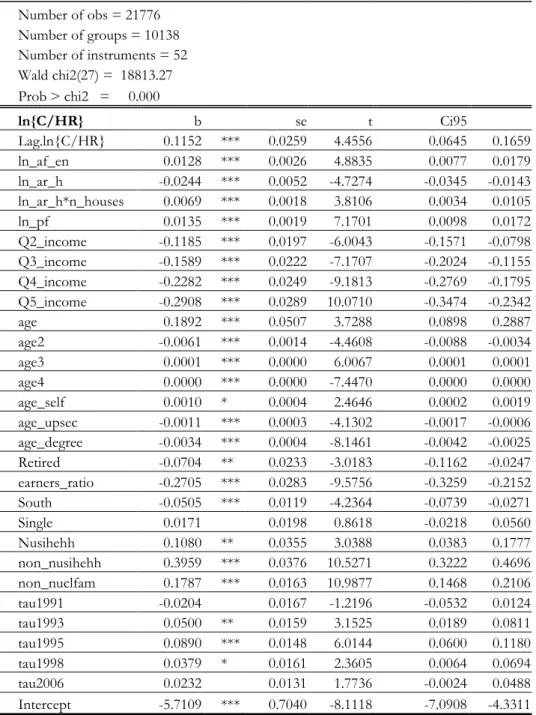
4. Estimation of the consumption rule

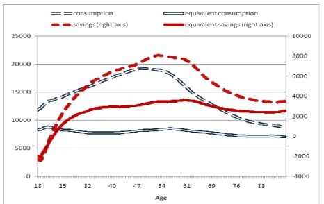
In this section we discuss the specification and the estimation of the consumption rule whose parameters we employ in the simulation program. As mentioned in the introduction, the idea that drives our approach is that the likely impact of radical social security reforms on the consumption/savings age profile of Italian households asks for a step beyond the estimation of a traditional reduced form Keynesian equation. In fact, if we look at the recent past (i.e. our 1991-2006 panel dataset, figure 7) through a set of kernel regressions, we notice that the (equivalent) savings profile of Italian Household is characterized by a quasi-flat pattern from around 35 onward, with pensioners having, on average, a positive propensity to save even at older ages.

38 _{Another assumption which improves the fit of our model is the expected residual life for the household (which in turn is}

equal to max between the residual lives of the two spouses, if any) can never be lower than five years. Therefore min tk

22

A broad literature has investigated the so called “retirement consumption puzzle” in several countries (Lunberg et al. 2001, Fernandez and Krueger, 2003 and 2004) and, for Italy, some authors explained - at least partially - the high (private) savings propensity of elderly with the generosity of the social security system (Miniaci et. Al, 2003) which, so far, provided pensioners with rather high rate of returns on contributions and high replacement rates. Once the social security wealth is included in the total wealth, the savings profile of Italian Households turn to be more consistent with the life cycle hypothesis, with a positive propensity up to retirement, and a spend down phase in the following period.39

Figure 7: Consumption and saving age profiles in the estimation dataset

Source: Author’s computations on SHIW 1991-2006, Nadaraya-Watson nonparametric regression, Euros 2002

We believe that thinking of this pattern as given and projecting it in the next decades - when social security reforms will be fully operational and the generosity of public pensions will be sensibly reduced - would miss an important part of the distributional story. In fact, reforms affect especially current young and future workers whose life cycle consumption is not or only partially observed and whose expectations have only partially embodied the long run effects of the reforms themselves. Therefore, we believe that linking consumption behavior to a life-cycle theoretical framework, while at the same time searching for a specification that fits more closely our data, is an appropriate strategy in order to account for such issues.

As mentioned in section 3., the empirical specification is the following:

( )

1 , 1 ' = ' ( ) ln ln t t t t t t h h h m m h h h t t m

Polynomial _{Households Current} Financial

lagged in age of the hh _{and hh Disposable} Ass

dependent and relative _{Characteristics Incomes}

interactions _Dummies C C pa D H y k AF HR

ρ

HR

δ

β

ψ

− + + +

∑

+ + ln ln (10) t t t h h h h House Financial

ets Equity Debt

AH PF u

ς

ϑ

ε

+ + + +

39 _{A drop in consumption after retirement still remains to be clarified. Several theoretical and empirical works propose}

different explanations for this stylized fact (Hurd and Rohwedder, 2008; Laitner and Silverman 2005; Fernandèz-Villaverde and Krueger, 2005. For Italy, Miniaci et al., 2009)

23

Such a functional form, where the dependent is (log of the) consumption to HR ratio, proves to better fit our household consumption data all over the distribution, while at the same time, considering the role of habit persistence40 _{and the effect of future expectations about incomes and pensions outcomes as a crucial} determinants of current consumption. Moreover, by estimating a propensity instead of a level, in the simulation program we get rid of the necessity to make arbitrary assumptions due to the non-stationarity of consumption which would have implied a moving average and therefore a dynamics in the intercept of the equation.

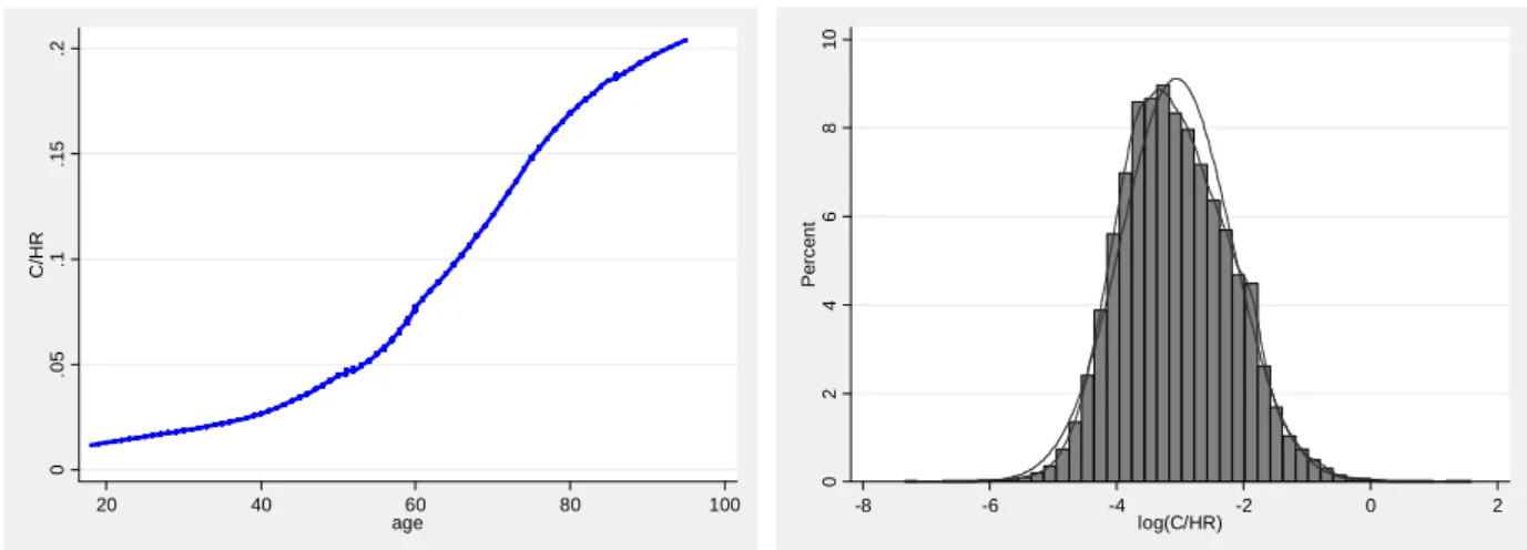
In the left panel of figure 8 we depict the lowess regression of the dependent variable over household head’s age in SHIW data (which increases non-monotonically) while in the right panel we check the distribution of its logarithm which is particularly well-behaved, closely approximating a normal distribution, with a slight right skewness.

Figure 8.: Consumption over human resources ratio: all households, lowess by age (left) and distribution (right)

0 .0 5 .1 .1 5 .2 C /H R 20 40 60 80 100 age 0 2 4 6 8 1 0 P e rc e n t -8 -6 -4 -2 0 2 log(C/HR)

Source: Author’s computations on SHIW 1991-2006, lowess regression (left) kernel distribution (right)

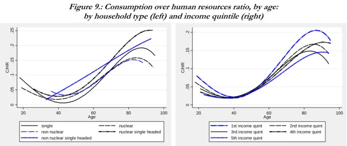
As a last exploratory analysis of our dependent variable, in figures 9 we show its average pattern, approximated by a cubic fit, by subgroups household types (left) and income quintiles (right). In particular, for the former, we divided the household population in five categories: singles, nuclear families (two spouses plus children, if any), non-nuclear families (households with spouses and active children only, not properly composite non-nuclear families41_{), nuclear single headed and non-nuclear single headed. As we can notice these household} types systematically differ each other in their propensity to consume out of their human wealth; therefore, controlling for them allows us to account for the effect of demography on consumption in our simulation program. Concerning income quintiles, we can notice a different consumption pattern related to current income, with, as expected, richer households saving more out of their human resources compared to low-income households.

40

We also estimate a static version of the model for new households with no lagged value of consumption to set the initial condition.

41 _{Consistently with the demographic hypotheses which ground CAPP_DYN, that is to simulate the evolution of the Italian}

population allowing for nuclear families only, we dropped the household with a non-nuclear, composite structure by the econometric analysis.