Weather Derivatives as Risk Management Tool in Ecuador: A Case Study of Rice Production

Weather Derivatives as Risk Management Tool in Ecuador:  

A Case Study of Rice Production 

Dmitry Vedenov

 and Leonardo Sanchez

bPhD student, Texas A&M University, [email protected] 

Selected Paper prepared for presentation at the Southern Agricultural Economics Association

Annual Meeting, Corpus Christi, TX, February 5-8, 2011

Copyright 2011 by Vedenov and Sanchez.  All rights reserved.  Readers may make verbatim copies of this  document for non‐commercial purposes by any means, provided that this copyright notice appears on all  such copies. 

Introduction 

Rice is one of the largest cereal crops in Ecuador. It is cultivated on the coast and employs 11% of labor 

force in agriculture. The provinces of Guayas and Los Rios produce 47% and 40%, respectively of the 

Ecuador total production of rice. Together these two provinces account for 83% of hectares planted with 

rice. 

According to the 2000 Census, 45% of the production units (UPA1) that are dedicated to rice production 

have at most 5 hectares, and 75% of the UPA's are small producers with less than 20 hectares.  

Ecuador exports rice mainly to Colombia, Peru and Venezuela. The volume of the rice trade does not 

exhibit a sustained trend over time. Rather, it depends on domestic supply, domestic producer price 

paid relative to exports, the supply situation in neighboring countries, and formal and informal current 

regulations at the northern and southern borders regarding the trade of rice. 

The existing price support policy contributes to distortions in Ecuadorian rice market. In 2009, the 

government of Ecuador signed the ministerial agreement No.0071 with the rice producers, which 

established a price support for rice at USD 28 per a 200‐pound bag. The policy is used to guarantee a 

minimum price in case of overproduction, with the government buying excess rice in order to keep the 

price at the established level. A government agency — Unidad Nacional de Almacenamiento2 (UNA) —

was created to provide a nationwide network of grain storage that would meet the domestic 

requirements and also serve as a resource in times of surplus production in order to supply international 

markets. 

However, small farmers do not always benefit from this policy. When the government purchases rice 

due to overproduction, the producers must bring their production to UNA in order to receive the 

support price. Small farmers usually do not have access to the infrastructure to bring their rice to the 

storage units. Thus, they lose the opportunity to receive the price at the support level. On the other 

hand, the farmers borrow money to cover their planting cost. Intermediaries who lend them money 

then buy small farmers’ production at a lower price than the price support. 

1 _{UPA stands for Unidad Productiva Agropecuaria (Agricultural Production Unit).}  2

There are other threats to small farmers’ well‐being. The extreme weather often affects rice yields in 

Ecuador. During the winter season (February and March) excessive rains could affect the growth of the 

plant. When El Niño occurs rains become more intensive. On the other hand, low temperatures are 

primary concerns during the summer season (August and September), especially with La Niña. 

Agronomists have observed evidence of relationship between low rice yield and El Niño events. Figure 13 

shows that both cereal GDP and Agricultural GDP4 fell as a result of El Niño in 1998. In the years 

preceding the 1998 El Niño, cereals represented 13.1% of the total agricultural GDP, while after the El 

Niño, they only contributed 9.56%. This is just one example of how extreme weather event could push 

rural and smallholder farm households into a cycle of poverty (Skees, 2008), especially when they have 

poor access to infrastructure. 

Since Ecuador lacks both the traditional crop insurance and general insurance markets, weather 

derivatives, if appropriately designed, could be used as risk management tools for rice production. 

Literature Review 

In the last two decades the literature about weather index contracts has grown significantly (Skees, et 

al., 2001; World‐Bank, 2005; Barnett,Barrett and Skees, 2008). However, the idea is not new. In 1943 the 

Congress of The United States decided to liquidate the federal crop insurance system. According to 

Sanderson, 1943), the high‐risk on wheat production and the considerable underwriting losses were the 

main reasons. At that time, Sanderson argued that the failure of the crop insurance program was not 

due to unfavorable weather. It was caused by a mixture of mismanagement and perverse incentives 

created by the program. Thus, he suggested that the success of any weather contract would depend on: 

“(1) on the correlation existing between the weather factors included in the estimating equation and the 

state average yield, and (2) on the degree of similarity in the response of individual‐farm yields to 

fluctuations in these weather factors”5. 

More recent, studies have divided their attention between two aspects — the design and pricing of 

weather contracts, and the risk‐reducing effectiveness of these.  

       3

 Figures 3 and 4 display the evolution of rice production for winter and summer respectively. 

4 _{Central Bank of Ecuador reports that rice and corn together represents around 80% of cereal GDP. For that}  reason, any bad event on rice production makes cereal GDP moves down. 

5

In 1980s, the Federal Crop Insurance Program consistently reported poor actuarial performance and a 

low participation rate. Miranda, 1991) argued that the problems were caused because the Federal Crop 

Program tried to tailor coverage to individual farmer yield losses.  He proposed that the individual 

producer yield risk can be divided into a systemic risk and a nonsystemic risk6. Because the nonsystemic 

part is extremely expensive to measure, Miranda suggests that a Federal Program (what he calls area‐

yield crop insurance) should cover only the systemic part. To illustrate his ideas, he used farmer level 

yield data for 102 soybean producers in the state of Kentucky.  Using empirical yield distributions he 

concluded that the area‐yield program tends to reduce farmers’ risk exposure. However, he warns that 

this program could not be widely accepted.  

Skees,Black and Barnett, 1997) discuss the procedures used in the Group Risk Plan to design and rate 

the area yield crop insurance contract.  They point out that area yield program (AYP) can be improved in 

many ways. They pay attention in the county boundaries as a way to reduce basis risk. Also, they argued 

that a better contract design could improve the AYP performances, and AYP will work in areas where 

yield risks are largely systemic. 

Earlier studies have also analyzed how effective weather derivatives are in reducing risk exposure, 

especially if some effort is made to minimize the basis risk (Turvey, 2001). Martin,Barnett and Coble, 

2001) propose an insurance instrument for cotton in Mississippi, which gives more flexibility to the 

purchasers because they are allowed to choose the parameters of the contract according to their risk 

management needs. Their results encourage the use of weather derivatives within the US agriculture. 

Turvey (2001) examines the pricing of weather derivatives in Ontario. He finds that specific‐event 

weather conditions affect crop yield risk. His results show that pricing a weather derivative on large area 

would be inadequate. He also points out to the need to minimize basis risk. 

Vedenov and Barnett, 2004) evaluate the efficiency of weather derivatives for three crops in The United 

States. The relationship between yield and weather variables is estimated using alternatives 

specifications. Using the data for six crop reporting districts, they construct “elementary” contracts for 

each district. They find the weather insurance contracts to differ across regions and crops, but the 

designed contracts do provide risk protection against yield shortfalls. 

       6

Deng,Barnett and Vedenov, 2007) analyze the risk reduction performance of an index contract and a 

farm‐level contract7 for cotton and soybean production for heterogeneous regions in Georgia and South 

Carolina. They argue that actuarially fair premium rates commonly used to compare both programs 

tends to bias results in favor of MPCI and therefore they use three different premiums rating schemes. 

Their results indicate that GRP performs better than MPCI not only within homogenous production 

region, but also with heterogeneous ones. They find that the GRP works well when MPCI premium rates 

are large and GRP basis risk is moderate. 

In developing countries, informal insurance and credit markets have been characterized by high interest 

and premiums rates. Nonmarket institutions8  (such as family, local, or community lending institutions) 

have been utilized as informal risk transfer mechanisms in rural areas of developing countries. Informal 

loans, diversification of income sources, and crop diversification have been mechanisms used by rural 

household to smooth consumption (Morduch, 1995; Fafchamps and Lund, 2003). In some cases, these 

systems have been better able to address the asymmetric information and transaction costs problems 

than formal insurance markets  (Stiglitz, 1990; Barnett,Barrett and Skees, 2008). 

However, when an extreme weather event makes farmers' losses correlated, these nonmarket 

institutions fail as risk management tool and as mechanism to avoid poverty traps (Zimmerman and 

Carter, 2003; Hess, et al., 2005; Santos and Barrett, 2006). In general, both governments and rural 

household of developing countries have not been effective managing risk transfer neither ex‐ante nor 

ex‐post of a shock (Carter and Barrett, 2006; Carter, et al., 2007; Barnett,Barrett and Skees, 2008). 

In recent years, weather derivative products have also been used in developing countries as a way to 

reduce the negative impacts of natural disasters. For example, Skees, et al., 2001) develop a rainfall‐

based index insurance in Morocco. Focusing on the three main cereal crops, they find a basic cumulative 

rainfall contract could reduce basis risk for cereal, and at the same time provide income protection to 

farmers.  They argue that this type of contracts is feasible in the more favorable agro climatic zones, 

where data reveal strong correlation between rainfall and cereal revenues. They conclude that a new 

program based on this type of insurance would make farmers better off. 

Data  

7 _{GRP (Group Risk Program) and MPCI (multiple peril crop insurance), respectively.}  8

The province of Guayas and Los Rios produces around 87% of the total rice production. In this study we 

focus on the information reported for two counties: Daule and Babahoyo, which are located in Guayas 

and Los Rios respectively. The county‐level rice data per season are obtained from MAGAP in the period 

1990‐2008. MAGAP reports the total rice production for each county.  

The county‐level weather data used for analysis are observations of average monthly total rainfall and 

temperature for the two winter months (February and March) and two summer months (August and 

September). Data for each weather station are collected from databases of the Instituto Nacional de 

Meteorología e Hidrología9 (INAMHI) which gather this information from the weather stations located in 

both provinces. 

Data Exploration 

According to MAGAP, since 2000 these two counties have represented more than 35% of rice 

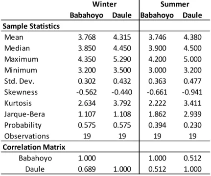
production in Ecuador. Descriptive statistics of the collected data are presented in Table 1. The table 

provides basic information about these counties. Figures 1‐2 present historical rice yields in each county. 

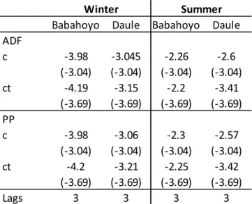
Two unit root tests — Augmented Dickey‐Fuller and Phillip‐Perron — were performed on the data (Table 

2). The test results suggest that there is no evidence of unit root in all counties in both seasons. 

Detrending Data 

The historical yield graphs in Figure 1‐2 9 also suggest that the rice production is affected by a trend. To 

account for this effect, yields and weather data are detrended using a log‐linear trend model: 

1990  

The detrended yields were calculated as: 

Yield‐Weather Relationship 

       9

The weather models used to define the weather index are constructed based on the relationship 

between rice yield and weather variables. As mentioned above, winter production is affected mainly by 

rainfall, while low temperatures are the primary concern during the summer. Tables 2 and 3 list weather 

models estimated as a part of the preliminary analysis. Of the models analyzed, the best one has a 

goodness of fit of only R2 = 0.33 (for Babahoyo in winter season).  

Design and Pricing of Weather Derivatives 

Following Vedenov and Barnett (2004), a weather derivative is modeled as an “elementary contract” 

with the payoff according to the schedule: 

(1)   | , ∗_, 0   ∗ ∗ ∗ ∗      ∗ ∗   1   ∗  

where   is a realization of the index. The contract starts to pay when the index   falls below the 

specified “strike”  ∗. Once the index falls below the limit  ∗, the insured receives the maximum 

indemnity  . When the index falls between the strike and the limit, the contract pays a proportion of the 

maximum indemnity. The parameter  varies between 0 and 1, with the limiting case of 0 corresponding 

to the conventional proportional payoff with deductible, and 1 corresponding to a “lump‐sum” payment 

once the contract is triggered regardless of the severity of the shortfall. The contract is completely 

designed once the values of strike, limit and maximum indemnity are specified (See Figure 3). 

In order to price the designed contract for a given set of parameter values, the probability distribution 

 of the index should also be specified. Using historical weather observations from each selected 

location, the weather‐yield models are used to calculate the “historical realizations” of the index for 

each location. In this study it is assumed that the index can be modeled with a normal probability 

function.   

The actuarially‐fair premium is set equal to the expected payoff of the contract, i.e.  

The parameters in equation (1) are selected for each location/index analyzed so as to provide the 

maximum risk reduction for the buyers who are exposed to the risk area‐wide yield loss. In particular, 

the parameters are selected so as to maximize the expected utility  

(3)      _{, , ∗}  | , ∗_{, ,} ∗_,  

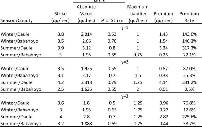
The strikes, limits, and maximum liabilities for optimal contracts are reported in table 5. A CRRA10 power 

function was used to get the parameters on the contracts 

(4)       ;  

The weather models estimated (table 4) suggest that each season/county combination has its own index 

and the models fail to capture the relationship between weather and yields. The result shown in table 5 

suggests that weather derivatives vary across county and season (e.g. Daule during the winter vs Daule 

during the summer). Thus, location, season, edaphology, and agricultural practices imply the need for 

different weather derivatives.  

Efficiency Analysis 

The risk‐reducing effectiveness of weather derivatives as a risk management tool was evaluated using 

the certainty‐equivalent revenue. It is assumed that an economic agent (a representative farmer or a 

“risk aggregator”) who is exposed to rice yield risk in a given seasons buys the weather derivative for the 

season.   The agent is considered a price taker and therefore only affected by the yield risk.  

For each location/season combination, the revenues without and with the contract were calculated as 

(5)    

(6)   | , ∗_{, ,} ∗_,  

where   is the (fixed) rice price. The expected revenues were then obtained as 

(7)        

       10

(8)   ∬ | , ∗_{, ,} ∗_{, ,}      

Where   and  ,  are the univariate and joint density function, respectively. The univariate 

density functions for each location/season combination were estimated using a normal distribution. The 

joint distributions of indices and yields were estimated using a Gaussian Copula  (Wand and Jones, 1995; 

Cherubini,Luciano and Vecchiato, 2004; Vedenov and Power, 2008) 

The expected utilities of revenues without and with the weather derivatives were calculated as 

(9)        

(10)   ∬ | , ∗_{, ,} ∗_{,   ,}      

For a given level of risk premium  and each revenue/location/season distribution, the parameter  was  

calibrated to be equal to 1, 2, and 3, so as to reflect producers’ willingness to forgo a certain amount of 

“risk‐premium” in exchange for elimination of uncertainty in the baseline case (without the insurance).  

The certainty‐equivalent revenues without and with the weather contract were calculated from the 

conditions, 

(11)    

(12)    

Finally, the risk reduction due to the weather derivative was computed as Δ

.Table 6 shows the results of this procedure. 

Results 

Risk‐reducing efficiency of weather derivatives as primary insurance instruments varies across county 

and season. In all cases the risk reduction is less than 1% except for Daule during the summer when the 

The risk reduction is small, apparently the poor performance of the weather models to capture the 

relationship between yields and weather is one of the reasons. Producers would not gain much if they 

buy the contract. The higher of value for  , the more risk reduction producers get 

Conclusion 

The efficiency of weather derivatives was analyzed for rice production in two counties during two 

seasons. For each county/season combination, the relationship between yield and selected weather 

variables was estimate for alternative functional forms, and a weather derivatives was constructed 

based on the function which best fit the data. This analysis was conducted using yields measured at 

county level. The constructed weather derivatives provided a little risk protection, apparently due to the 

high basis risk.   

References 

Barnett, B.J., Barrett, C.B., and Skees, J.R. "Poverty Traps and Index‐Based Risk Transfer Products" World 

Development 36, 10(2008): 20. 

Besley, T. "Nonmarket Institutions for Credit and Risk Sharing in Low‐Income Countries" The Journal of 

Economic Perspectives 9, 3(1995): 115‐127. 

Carter, M.R., and Barrett, C.B. "The Economics of Poverty Traps and Persistent Poverty: An Asset‐Based 

Approach" Journal of Development Studies 42, 2(2006): 178 ‐ 199. 

Carter, M.R., Little, P.D., Mogues, T., and Negatu, W. "Poverty Traps and Natural Disasters in Ethiopia 

and Honduras" World Development 35, 5(2007): 835‐856. 

Cherubini, Luciano, and Vecchiato. Copula: Methods in Finance. Edited by John Wiley & Sons, L., 2004. 

Deng, X., Barnett, B.J., and Vedenov, D.V. "Is There a Viable Market for Area‐Based Crop Insurance?" 

American Journal of Agricultural Economics 89, 2(2007): 508‐519. 

Fafchamps, and Lund. "Risk Sharing Networks in Rural Philippines" Journal of Development Economics 

71, 2(2003): 27. 

Hess, U., Skees, J.R., Stoppa, A., Barnett, B.J., and Nash, J. "Managing Agricultural Production Risk: 

Innovations in Developing Countries."   No. 32727‐GLB. The World Bank, Washington, D.C. 

Available  online  at 

http://siteresources.worldbank.org/INTARD/Resources/Managing_Ag_Risk_FINAL.pdf. 

Martin, S.W., Barnett, B.J., and Coble, K.H. "Developing and Pricing Precipitation Insurance" Journal of 

Agricultural and Resource Economics. 26, (2001): 14. 

Miranda, M.J. "Area‐Yield Crop Insurance Reconsidered" American Journal of Agricultural Economics 73, 

2(1991): 233‐242. 

Morduch, J. "Income Smoothing and Consumption Smoothing" The Journal of Economic Perspectives 9, 

3(1995): 103‐114. 

Sanderson, F.H. "A Specific‐Risk Scheme for Wheat Crop Insurance" Journal of Farm Economics 25, 

Santos, P., and Barrett, C.B. "Heterogeneous Wealth Dynamics: On the Roles of Risk and Ability" SSRN  eLibrary (2006). 

Skees, J.R. "Innovations in Index Insurance for the Poor in Lower Income Countries" Agricultural and 

Resource Economics Review 37, 1(2008): 15. 

Skees, J.R., Black, J.R., and Barnett, B.J. "Designing and Rating an Area Yield Crop Insurance Contract" 

American Journal of Agricultural Economics 79, 2(1997): 430‐438. 

Skees, J.R., Gober, S., Varangis, P., Lester, R.R., and Kalavakonda, V. "Developing Rainfall‐Based Index 

Insurance in Morocco" SSRN eLibrary (2001). 

Stiglitz, J.E. "Peer Monitoring and Credit Markets" The World Bank Economic Review 4, 3(1990): 16. 

Turvey, C.G.  "Weather Derivatives for Specific Event Risks in Agriculture" Review of Agricultural 

Economics 23, 2(2001): 333‐351. 

Vedenov,  D.V.,  and  Barnett,  B.J.  "Efficiency  of  Weather  Derivatives  as  Primary  Crop  Insurance 

Instruments" Journal of Agricultural and Resource Economics. 29, 3(2004): 17. 

Vedenov, D.V., and Power, G.J. "Risk‐Reducing Effectiveness of Revenue Versus Yield Insurance in the 

Presence of Government Payments" Journal of Agricultural and Applied Economics 40, 2(2008): 

17. 

Wand, M.P.,  and Jones, M.C. Kernel Smoothing.  Vol. 60. Monographs  on Statistics and  Applied 

Probability. Edited by Hall/CRC, C. London, 1995. 

World‐Bank. "Managing Agricultural Production Risk: Innovations in Developing Countries." Agricultural 

and Rural Development Department, The World Bank, Washington, D.C. Available online at. 

Zimmerman, F.J., and Carter, M.R. "Asset Smoothing, Consumption Smoothing and the Reproduction of 

Inequality under Risk and Subsistence Constraints" Journal of Development Economics 71, 

2(2003): 233‐260.                   

Figure 1: Dynamics of Rice Production in Babahoyo, 1990‐2008      2.5 2.7 2.9 3.1 3.3 3.5 3.7 3.9 4.1 4.3 4.5 1990 1991 1992 1993 1994 1995 1996 1997 1998 1999 2000 2001 2002 2003 2004 2005 2006 2007 2008 Rice   Yi el d,    Me tr ic   To ns   /H ec ta re Winter Summer

Figure 2: Dynamics of Rice Production in Daule, 1990‐2008      2.5 3 3.5 4 4.5 5 5.5 1990 1991 1992 1993 1994 1995 1996 1997 1998 1999 2000 2001 2002 2003 2004 2005 2006 2007 2008 Ri ce   Yie ld ,   Me tr ic   To ns   /   Hec ta re Winter Summer

Figure 3: Payoff Schedule for a Weather Derivatives Contract   

$ 0

0.5





….

Coinsurance

with

deductible,



=0.0

‐‐‐

Coinsurance

with

deductible

and

limit

on

some

payment,



=0.5

Lump

Sum,



=1.0

$x

We

at

h

er

De

ri

va

ti

ve

s

Pa

yo

ff

Weather 

Index

Table 1: Descriptive Statistics of Rice Yields for Main Producing Counties 

Babahoyo Daule Babahoyo Daule

Sample Statistics  Mean 3.768 4.315 3.746 4.380  Median 3.850 4.450 3.900 4.500  Maximum 4.350 5.290 4.200 5.000  Minimum 3.200 3.500 3.000 3.200  Std. Dev. 0.302 0.432 0.363 0.477  Skewness ‐0.562 ‐0.440 ‐0.661 ‐0.941  Kurtosis 2.634 3.792 2.222 3.411  Jarque‐Bera 1.107 1.108 1.862 2.939  Probability 0.575 0.575 0.394 0.230  Observations 19 19 19 19 Correlation Matrix Babahoyo 1.000 1.000 0.512 Daule 0.689 1.000 0.512 1.000 Winter Summer

Table 2: Unit Root Tests of Yield Data Series                 

Babahoyo Daule Babahoyo Daule

ADF c ‐3.98 ‐3.045 ‐2.26 ‐2.6 (‐3.04) (‐3.04) (‐3.04) (‐3.04) ct ‐4.19 ‐3.15 ‐2.2 ‐3.41 (‐3.69) (‐3.69) (‐3.69) (‐3.69) PP c ‐3.98 ‐3.06 ‐2.3 ‐2.57 (‐3.04) (‐3.04) (‐3.04) (‐3.04) ct ‐4.2 ‐3.21 ‐2.25 ‐3.42 (‐3.69) (‐3.69) (‐3.69) (‐3.69) Lags 3 3 3 3 Winter Summer

Note:The va ri a bl es a re expres s ed i n l oga ri thms . La gs i s 

the number tha t mi ni mi ze the Schwa rtz cri teri o. ADF= 

Table 3: Weather Models for Winter Season Based on 1990‐2008 Data                  Babahoyo Daule Rainfall February 0.00704 0.0110 (0.0313) (0.0426) Rainfall March 0.225 0.0390 (0.154) (0.104)

Rainfall February square ‐0.00183 ‐0.00209

(0.00267) (0.00446)

Rainfall March square ‐0.0155 ‐0.00400

(0.0121) (0.00793)

Constant 0.570 1.388***

(0.471) (0.284)

Observations 19 19

R‐squared 0.334 0.199

Standard errors in parentheses

*** p<0.01, ** p<0.05, * p<0.1

Table 4: Weather Models for Summer Season Based on 1990‐2008 Data                Babahoyo Daule Temperature August 4.816 ‐6.222 (9.313) (16.19) Temperature September ‐11.71 8.533 (13.55) (20.47)

Temperature August square ‐0.0302 0.0417

(0.0596) (0.109)

Temperature September square 0.0742 ‐0.0572

(0.0865) (0.137) Constant 271.8 ‐85.13 (322.9) (317.6) Observations 19 19 R‐squared 0.186 0.029 Summer

Standard errors in parentheses

Table 5: Parameters of Optimal Weather Instruments            Season/County Strike  (qq/hec) Absolute  Value  (qq.hec) % of Strike Maximum  Liability  (qq/hec) Premium  (qq/hec) Premium  Rate Winter/Daule 3.8 2.014 0.53 1 1.43 143.0% Winter/Babahoyo 3.5 2.66 0.76 1 1.54 146.3% Summer/Daule 3.9 3.12 0.8 1 3.34 317.3% Summer/Babahoyo 3 1.95 0.65 0.75 0.26 22.1% Winter/Daule 3.5 1.925 0.55 1 0.87 87.0% Winter/Babahoyo 3.1 2.17 0.7 1.5 0.38 25.3% Summer/Daule 4.2 3.318 0.79 1.25 4.14 331.2% Summer/Babahoyo 2.5 1.625 0.65 2 0.01 0.5% Winter/Daule 3.6 1.8 0.5 1.25 0.96 76.8% Winter/Babahoyo 3 1.95 0.65 1.75 0.22 12.6% Summer/Daule 4 2.8 0.7 1.25 2.82 225.6% Summer/Babahoyo 3.2 1.888 0.59 0.75 0.44 58.7% Limit =3 =1 =2

Table 6: Efficiency of Weather Derivatives as Measured by Certainty Equivalent            Season/County With Contract  (qq/hec) Without  Contract  (qq/hec) Percent  Change With Contract  (qq/hec) Without  Contract  (qq/hec) Percent  Change With Contract  (qq/hec) Without  Contract  (qq/hec) Percent  Change Winter/Daule 1.943 1.95 ‐0.4% 1.988 1.996 ‐0.4% 2.032 2.045 ‐0.6% Winter/Babahoyo 1.929 1.93 ‐0.1% 1.959 1.969 ‐1.0% 1.996 2.007 ‐1.1% Summer/Daule 1.922 1.931 ‐0.5% 1.956 1.969 ‐1.3% 1.979 2.007 ‐2.8% Summer/Babahoyo 1.946 1.946 0.0% 1.988 1.988 0.0% 2.026 2.03 ‐0.4% =2 =1 =3