Dispersion in Options Traders Expectations and Stock Return Predictability

Dispersion in Options Traders’ Expectations and Stock

Return Predictability

∗

Panayiotis C. Andreou

Anastasios Kagkadis

Paulo Maio

Dennis Philip

April 2015

∗_{We would like to thank Yakov Amihud, Turan Bali, Suleyman Basak, Stephen Brown, Frankie}

Chau, George Constantinides, Damian Damianov, Gregory Eaton, Bruce Grundy, Hui Guo, Madhu Kalimipalli, Neil Kellard, Eirini Konstantinidi, Robert Korajczyk, Alexandros Kostakis, Yuehao Lin, Hao Luo, Hong Luo, James Mitchell, Bradley Paye, Ilaria Piatti, David Rapach, Esther Ruiz, Fabio Trojani, Masahiro Watanabe, Hao Zhou and seminar and conference participants at Athens University of Economics and Business, Nottingham University Business School, MFS Symposium, Arne Ryde 2014 Workshop (Lund University), EFMA 2014 Meeting, Modelling Macroeconomic and Financial Time Series Conference (Loughborough University), NFA 2014 Conference, FMA 2014 Meeting, Paris 2014 Finance Meeting and MFA 2015 Meeting for helpful comments and suggestions. We are also grateful to Kenneth French, Amit Goyal, Martin Lettau, Robert Shiller and Hao Zhou for making data available on their websites. A previous version of this paper was circulated under the title “Stock Market Ambiguity and the Equity Premium”. Any remaining errors are our own.

†_{Department of Commerce, Finance and Shipping, Cyprus University of Technology, 140, Ayiou}

Andreou Street, 3603 Lemesos, Cyprus; Email: [email protected]

‡_{Durham University Business School, Mill Hill Lane, Durham DH1 3LB, UK; Email:}

[email protected]

§_{Department of Accounting and Finance, Lancaster University Management School, Lancaster}

LA1 4YX, UK; Email: [email protected]

¶_{Hanken School of Economics, P.O. Box 479, 00101 Helsinki, Finland; Email:}

Abstract

We propose a measure of dispersion in options traders’ expectations about future stock re-turns by using the dispersion in trading volume across strike prices. An increased dispersion in expectations forecasts lower excess market returns at both short and long horizons, while its out-of-sample predictability is both statistically and economically significant. The sug-gested dispersion measure is highly correlated with the dispersion in analysts’ forecasts but it consistently exhibits a stronger predictive ability. Further, it exhibits additional predic-tive power when combined with the variance risk premium, showing that the two variables capture different aspects of the variation in returns.

JEL Classification: G10, G11, G12, D81

Keywords: Dispersion in beliefs; Disagreement; Ambiguity; Predictability of stock returns;

Equity premium; Trading volume dispersion; Out-of-sample predictability; Economic signif-icance

1

Introduction

A growing body of studies has shown that various measures of dispersion in expectations can provide significant stock return predictability at both an individual and an aggregate level. There are two main strands in this literature. A first stream of papers assumes a het-erogeneous investors framework and uses dispersion to proxy for the level of disagreement among market participants (e.g. Diether, Malloy and Scherbina, 2002; Yu, 2011; Jiang and Sun, 2014). Disagreement can affect asset returns either due to the existence of trading fric-tions in the market or by inducing investors to engage into risk-sharing acts that affect asset prices in equilibrium. A second strand of the literature assumes a homogeneous investors framework and uses dispersion to proxy for the level of ambiguity perceived by investors (e.g. Anderson, Ghysels and Juergens, 2009; Drechsler, 2013). Ambiguity can affect asset returns due to the fact that naturally investors exhibit aversion to events with unknown probability distributions.

In this paper, we explore the information content of the dispersion in options traders’ expectations for future market excess returns. To this end, we construct a novel dispersion in expectations measure that is represented by the dispersion in the volume-weighted strike prices of equity index option contracts. In light of this, a high dispersion of trading volume across strike prices is associated with a high dispersion in beliefs in the options market and vice versa.

The suggested measure is motivated by a simple theoretical framework within which op-tions end-users engage in trading activities with market makers driven by their expectaop-tions about the future price of the underlying asset. We posit that in such a case the expected returns of the end-users are naturally reflected in the strike prices at which the options trad-ing strategies are implemented. For example, the obvious choices for an optimistic investor would be either to buy a call option or sell a put option. In the first case, an increase in the asset price increases the investor’s final payoff, while in the second case it ensures that the option will not be exercised at maturity and the investor will secure the option premium. In

addition, the more optimistic the investor, the higher the strike price she will choose. This is because an out-of-the-money (OTM) option has a lower premium and exhibits a higher lambda1 _{than an in-the-money (ITM) option. Therefore, a call buyer (put seller) will be} inclined to select a strike price that is as low as possible in order to ensure that the call will be exercised (the put will expire worthless), but is as high as possible in order to benefit from the higher lambda (higher premium). Therefore, due to this trade-off the selected strike price will reflect the investor’s expectation about the future underlying asset price, in the sense that a more positive expectation will result in a trade at a more OTM call or a more ITM put option.2

Furthermore, the put-call parity suggests that an optimistic investor can replicate the payoff from buying a call option (selling a put option) by borrowing at the risk-free rate and buying a put option and the underlying asset (selling a call option and buying the underlying asset). Therefore, by inverting the argument above, it is easy to see that a more positive expectation will be associated with a trade at a more ITM put or a more OTM call. The above arguments can be easily reversed and hold for the case of a pessimistic investor as well. Moreover, the arguments can be extended to the case of more complicated trading strategies (e.g. call or put spreads and backspreads), since such strategies can be decomposed into a series of simpler ones. As a result, the overall expectation implied by such a strategy can be seen as an aggregation of the different expectations implied by the simpler ones. The above discussion illustrates that any option trade can be theoretically linked to a specific expected return through the strike price at which it was implemented.

Compared to prior studies, which develop dispersion in beliefs measures based on ana-lysts’ forecasts or mutual fund and individual investor portfolio holdings,3 _{the dispersion in} 1_{The lambda (or leverage) of an option is the elasticity of the option price to changes in the underlying}

asset price. It is defined as the ratio of the percentage change in the option price to the percentage change in the underlying asset price.

2_{In practice it is possible that other factors such as market liquidity or limits to arbitrage may play some}

additional role in the options positions taken. To the extent, however, that options trading ismainly driven by traders’ expected asset returns, the framework described here is reasonable.

3_{Diether, Malloy and Scherbina (2002); Park (2005); Anderson, Ghysels and Juergens (2005, 2009); Yu}

options traders’ expectations exhibits several advantageous characteristics. First, it stems from all the trades that take place in a highly liquid options market, thus capturing all the expectations that are considered probable enough to trigger a trade.4 _{In contrast, analysts’} forecasts constitute only a limited set of opinions,5 _{and have been found to be affected by} agency issues between firms and investment banks and to be prone to analysts’ behavioral biases (Dechow, Hutton and Sloan, 2000; Daniel, Hirshleifer and Teoh, 2002; Cen, Hilary and Wei, 2013). Second, it is directly related to expected returns, while analysts’ predictions refer to alternative economic indicators such as corporate earnings and hence supplementary modeling assumptions are needed to derive expectations about returns. Third, unlike dis-persion measures constructed from analysts’ forecasts or mutual fund holdings data, it can be estimated on an even higher frequency than monthly or quarterly, thus providing a much more realistic picture of the evolution of dispersion in expectations across time. Moreover, the Chicago Board Options Exchange (CBOE) provides freely on its website the intraday trading activity of option contracts, thus making it easy for investors to use the dispersion in options traders’ beliefs measure for investment decisions. Fourth, our measure can equally accommodate optimistic and pessimistic beliefs since it is hardly influenced by the short-sale constraints present in the equity market that affect both individual and institutional investor portfolio holdings.6 _{Finally, it can explicitly distinguish between different levels of} positive and negative expectations, while this is not straightforward in the case of dispersion measures derived from investors’ positions in the equity market.

Our results establish a significant and robust negative relationship between the dispersion in options traders’ beliefs and future market returns. In particular, an in-sample regression while Chen, Hong and Stein (2002); Goetzmann and Massa (2005) and Jiang and Sun (2014) create dispersion measures from mutual fund and individual investor portfolio holdings.

4_{The available range of strike prices for index options is determined by the underlying index fluctuations}

and the customer requests. CBOE Rule 24.9.04 specifies that typically strike prices for index options should be within 30% of the current index value, but even more extreme strike prices are permitted provided there is demonstrated customer demand.

5_{For example, the average number of forecasters in Anderson, Ghysels and Juergens (2009) is 36.} 6_{Almazan, Brown, Carlson and Chapman (2004) provide evidence showing that approximately only 3%}

analysis shows that at the 1-month horizon, the suggested measure of dispersion in expecta-tions is a strong predictor of future excess market returns under various model specificaexpecta-tions (univariate and multivariate). Moreover, it outperforms in terms of predictive power all other predictors examined in prior literature apart from the variance risk premium (VRP), which explains a higher proportion of the variation in future returns. In addition, it offers addi-tional predictability when combined with VRP in the same forecasting model, thus showing that the two variables have different information content and can be used complementarily for predicting future market returns.7 The results from long-horizon regression analysis show that our dispersion in beliefs measure remains significant at all horizons, and for horizons of 12 and 24 months ahead exhibits an adjustedR2 _{higher than 10%, outperforming the} major-ity of the alternative predictors. It is also important to note that while it is highly correlated (about 60%) with the dispersion in analysts’ forecasts measure (AFD) of Yu (2011), its long-horizon predictive ability is clearly superior to that of the dispersion in analysts’ forecasts. The above results are noteworthy because unlike AFD and the majority of the other pre-dictors, the dispersion in options traders’ expectations exhibits a relatively low persistence (about 0.50) hence alleviating potential concerns regarding spurious predictability.

The results of out-of-sample predictive analysis reveal that the dispersion of options traders’ beliefs has significantly higher forecasting power than the historical mean and it outperforms all other predictive variables (including the dispersion in analysts’ forecasts) apart from VRP. Following Campbell and Thompson (2008), imposing a constraint of posi-tive forecasted equity premia leads to further improvement of the out-of-sample predictability of dispersion in beliefs for the excess market return.

The results are also economically significant since an active trading strategy based on 7_{Compared to the VRP, which has emerged as the primary option-implied return predictor, the dispersion}

in options traders’ expectations is conceptually different. First, it is not extracted from option prices and therefore it is not derived from the risk-neutral distribution. Second, while the level of trading volume could potentially have an effect on option prices and subsequently on VRP in accordance with the limits to arbitrage hypothesis (Bollen and Whaley, 2004), high trading volume is not necessarily associated with high dispersion across different moneyness categories. Therefore, the market forces that influence VRP do not have an apparent effect on the dispersion in options trading volume across strike prices. In fact, the empirical analysis suggests that the correlation between the two measures is close to zero.

the out-of-sample predictive power of the proposed dispersion in expectations measure offers increased utility to a mean-variance investor that would otherwise follow a passive buy-hold strategy. Moreover, in terms of economic significance the dispersion in options traders’ expectations outperforms AFD as well as the rest of the predictors except for VRP in almost all the cases. It is therefore evident that the suggested dispersion in beliefs measure is superior to the traditional dispersion in analysts’ forecasts measure both in statistical and in economic terms. Furthermore, when combined with the VRP it improves the performance of a trading strategy that would otherwise rely solely on the VRP. Therefore, it is again confirmed that the dispersion of options traders’ opinions and the VRP act as complementary variables and their joint use for investment decisions can prove very beneficial to an active investor. The performance of rotation strategies that rely on the out-of-sample predictive power of the dispersion in beliefs measure for several equity portfolio excess returns reveal that its information content is economically important not only for the aggregate market but also for the majority of the portfolios sorted on different stock characteristics.

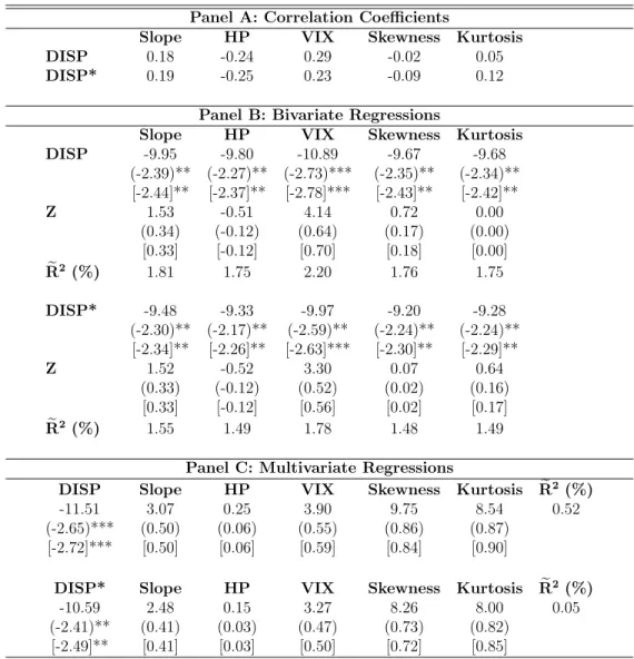
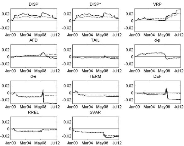
Finally, we compare the dispersion in options trading volume across strike prices with other popular option-implied variables in order to alleviate potential concerns about the in-formation embedded in our measure. More specifically, the alternative option-implied vari-ables include the slope of the implied volatility smirk, the risk-neutral variance, skewness and kurtosis, and the OTM puts to the at-the-money (ATM) calls open interest ratio proxying for investors’ hedging pressure. Higher dispersion in options traders’ beliefs is associated with higher variance, more negative skewness, higher kurtosis, a more negatively sloped volatility smirk, and less hedging pressure. However, the highest correlation coefficient, which is the one between our dispersion in expectations variable and risk-neutral variance, is only 0.29, revealing that the suggested measure does not proxy for any type of variance or tail risk and is not driven by the well-known hedging demand for OTM puts. Bivariate and mul-tivariate regression analysis confirms that in the presence of the alternative option-implied measures, the dispersion in options trading volume across strikes remains highly significant

in forecasting subsequent market returns at all horizons.

The documented negative relation between the dispersion in options trading volume across strikes and the equity premium allows for a dual interpretation. First, if dispersion proxies for the level of disagreement in the underlying asset market, then this finding is in line with the models of Miller (1977) and Scheinkman and Xiong (2003), who show that in the presence of short-sale constraints asset prices reflect only the views of the most optimistic investors, since pessimistic investors sit out of the market. Therefore, higher disagreement is accompanied by higher asset prices and lower subsequent returns. In the context of the aggregate market, the above limits-to-arbitrage explanation can be supported by the empirical findings of D’Avolio (2002) and Lamont and Stein (2004), who show that only a very limited fraction of the total stocks are actually sold short.

Second, as in Easley and O’Hara (2009, 2010) we can consider a framework wherein there are two types of participants in the underlying asset market: sophisticated investors who are exposed only to risk and unsophisticated investors who are exposed to both risk and ambigu-ity. If we assume that investors within each group are homogeneous and the unsophisticated investors update their views by observing (to some extent) the trading activity in the options market, then the dispersion in options trading volume across strikes can be regarded as a proxy for their perceived level of ambiguity regarding the true return-generating model. In such a case, an increase (decrease) in the dispersion of options trading volume across strikes will be associated with an increase (decrease) in the ambiguity of the unsophisticated in-vestors, but also with an increase (decrease) in the dispersion of ambiguity acrossall equity market participants, since sophisticated investors know the true probability measure and hence face no ambiguity. In light of this, the documented negative relation between disper-sion in options volume and future market returns is in line with the theoretical model of Cao, Wang and Zhang (2005) and the empirical evidence of Chapman and Polkovnichenko (2009), who show that in the presence of high dispersion in ambiguity, the investors who perceive the highest ambiguity will choose to leave the market. As a result, the risky asset

will be held and priced by the sophisticated investors who perceive zero ambiguity and hence demand a lower equity premium (see also Epstein and Schneider, 2010).

The remainder of the paper is structured as follows. Section 2 presents the theoretical framework. Section 3 describes the data and the construction of the main variables used in the study. Section 4 provides the empirical evidence from in-sample regression analysis. Section 5 discusses the results from out-of-sample regression analysis. Section 6 presents the economic significance of the out-of-sample empirical evidence. Section 7 presents the com-parison between the dispersion in options trading volume and other option-related variables. Finally, Section 8 concludes.

2

Theoretical Motivation

This section firstly presents the theoretical motivation within which the dispersion in trading volume across strike prices can be seen as a proxy for dispersion in expectations about future stock returns and secondly provides two alternative explanations for the negative relation between the dispersion in trading volume across strike prices and the equity premium.

2.1

Dispersion in trading volume across strike prices as a proxy

for dispersion in expectations

The rationale behind the measurement of the dispersion in options traders’ beliefs via the dispersion in options trading volume across strike prices can be supported within the context of the following simple framework. We assume that the options market is mainly comprised of two groups of participants: end-users who trade OTM and ITM (at-the-money and near-the-money) options to benefit from directional changes in the underlying asset price (changes in the volatility of the underlying asset),8 and market makers who provide liquidity to end-users by taking the opposite positions. In light of this, this section discusses how the strike prices 8_{At-the-money and near-the-money options exhibit the highest sensitivity to volatility changes and hence}

at which a wide range of simple and complicated options trading strategies are implemented can naturally reflect the expected stock returns by the end-users. While we cannot rule out the possibility that other factors such as liquidity or limits to arbitrage may play a role for the initiation of a number of trades, we posit that the measurement of the dispersion in options traders’ beliefs via the dispersion in options trading volume across strike prices is reasonable to the extent that OTM and ITM option trades are mainly driven by investors’ expectations about the future price of the underlying asset.

For example, the most natural choices for an investor who has a positive expectation about the future price of the underlying asset would be either to buy a call option or sell a put option. In the first case, an increased asset price increases the investor’s final payoff, while in the second case it ensures that the option will expire worthless and the investor will profit from the option premium. Moreover, the more positive the expectation of the investor, the higher the strike price she will choose. This is because an OTM option has a lower premium and exhibits a higher lambda (or leverage) than an ITM (or less OTM) option. Therefore, a call buyer (put seller) will be inclined to select a strike price that is as low as possible in order to ensure that the call will be exercised (the put will expire worthless), but is as high as possible in order to take advantage of the higher lambda (higher premium). This trade-off implies that the selected strike price should reflect the investor’s expectation about the future underlying asset price, i.e. the more positive the expectation the more OTM the call and the more ITM the put option.

Alternatively, an optimistic investor could buy a put and the underlying asset or sell a call and buy the underlying asset. If these strategies are financed by borrowing at the risk-free rate then by the put-call parity they replicate the payoffs from buying a call and selling a put respectively. In such a case, a put buyer (call seller) will be inclined to select a strike price that is as high as possible in order to ensure that the put will be exercised (the call will not be exercised), but is as low as possible in order to take advantage of the higher lambda (higher premium). Therefore, as before, the selected strike price will closely match

the investor’s expectation about the future underlying asset price, with a more positive expectation leading to a trade at a more ITM put and a more OTM call.

On the other hand, the natural choices for an investor who has a negative view about the future realization of the underlying asset price would be either to buy a put option or sell a call option. Alternatively, the put-call parity suggests that a pessimistic investor can buy a call and short the underlying asset or sell a put and short the underlying asset. If the strategies also involve investment in the risk-free asset then they replicate the payoffs from buying a put and selling a call option respectively. In any case, by inverting the previous arguments it is easy to observe that a trade at a more OTM put or a more ITM call can be associated with a more negative expectation about the future underlying asset price.

It is true that from the above potential strategies some are more likely to be used (and in fact are widely used by options traders) while others may be more rare (for example the strategies that involve shorting the underlying asset). However, the key point from the above discussion is that every trade at an OTM or ITM option can be theoretically linked to a specific positive or negative expectation about the future asset price depending on the value of the strike price. Therefore, since the OptionMetrics database does not provide information on whether a trade was motivated by a seller or buyer, we use the aggregate trading volume on each strike price to proxy for the number of traders that share a common expected return. Furthermore, the above arguments can be extended to the case of more complicated strategies. For example, a bull call spread involves buying a call option with strike priceX1 and selling a call option with strike priceX2, withX1 < X2. Given the fact that the investor will try to maximize the lambda of the low strike call that is bought and the premium of the high strike call that is sold, it follows that the range of values betweenX1 and X2 comprises the range of prices that the investor considers as most probable for the future. Therefore, the higher the level of this pair of strike prices, the more positive is the investor’s view. Consistent with this intuition, if this is the only trade that takes place in the market during a given day, our framework suggests that the expected future underlying asset price implied

by the trading activity in the options market is X2+X1

2 . The intuition is exactly the same if instead of going long the call spread the investor goes short or if instead of a bull call spread we consider a bull put spread, a bear call spread or a bear put spread. Moreover, similar conclusions can be drawn if we consider other strategies such as call and put backspreads or butterfly spreads. This is because every trading strategy can be decomposed into simpler ones and the overall expectation implied by the strategy can be seen as an aggregation of the expectations implied by the simpler strategies.

2.2

Dispersion in trading volume across strike prices and the

eq-uity premium

The dispersion in options traders’ expectations can have two interpretations. First, it can be considered a proxy of the disagreement among participants in the underlying asset market, similarly to the studies of Park (2005) and Yu (2011). Such a disagreement can have an impact on future asset returns either due to the existence of short-sale constraints (Miller, 1977; Scheinkman and Xiong, 2003) or due to risk-sharing effects that impact asset prices in equilibrium (Basak, 2000, 2005; Buraschi and Jiltsov, 2006). Second, as in Anderson, Ghysels and Juergens (2009) and Drechsler (2013), it can be regarded as a measure of the ambiguity perceived by a group of underlying asset market participants who have homo-geneous beliefs but do not know the true model governing returns. In particular, if the beliefs of these investors are driven at least partly by the trading activity in the options market,9 the dispersion in options traders’ expectations can serve as proxy for the set of alternative return-generating models that these investors are exposed to.10 In this case, a high (low) dispersion in options traders’ opinions implies that it is highly likely that these 9_{In fact, option-implied sentiment indicators such as the put-call trading volume ratio are widely used}

by investors for investment allocation decisions.

10_{This framework is intuitive, since expected market returns are driven by aggregate macroeconomic}

fac-tors that are easily observable and therefore the likelihood is rather low that different expectations (and hence trades) are induced by information asymmetry instead of different views regarding the return-generating model.

market participants exhibit high (low) ambiguity about the true return-generating model. Since investors on average exhibit ambiguity aversion, i.e. they are averse to events with unknown probability distributions of all possible outcomes (Ellsberg, 1961; Bossaerts, Ghi-rardato, Guarnaschelli and Zame, 2010), it follows that market discount rates should reflect investors’ aversion not only to risk but also to ambiguity (Epstein and Wang, 1994; Chen and Epstein, 2002; Ju and Miao, 2012; Drechsler, 2013).

The empirical evidence presented in the subsequent sections of this paper shows that higher (lower) dispersion in options traders’ expectations is associated with a lower (higher) equity premium. This can be interpreted in two ways. If the dispersion in options trading volume across strikes proxies for the level of disagreement in the equity market, the negative predictability is in line with the models of Miller (1977) and Scheinkman and Xiong (2003). In particular, in the presence of short-sale constraints, the price of a risky asset is determined by the valuations of the most optimistic investors, as pessimistic investors have no means to express their negative views and sit out of the market. Therefore, higher disagreement is associated with higher prices and subsequent lower returns.11 The above limits-to-arbitrage argument appears empirically well-founded, as D’Avolio (2002) reports that only 7% of the total short-sale capacity is actually used, and Lamont and Stein (2004) show that during the period 1995-2002 the ratio of the market value of shares sold short to the total value of shares outstanding always remains below 4%.

If the dispersion in options trading volume across strikes is regarded as a proxy for the ambiguity faced by a homogeneous group of equity market investors, the negative predictabil-ity can be rationalized within the context of an economy similar to that analyzed by Easley and O’Hara (2009, 2010). In particular, we can assume that the equity market comprises two different groups of investors with investors within each group sharing common beliefs: the first group consists of sophisticated investors who know the true probability distribution 11_{A possible counterargument is that during periods of binding short-sale constraints investors would try}

to take advantage of the put-call parity arbitrage opportunities that would occur due to the overpriced un-derlying asset and hence the mispricing would immediately vanish. However, Grundy, Lim and Verwijmeren (2012) do not find any support for this hypothesis when examining the 2008 short-sale ban in the U.S.

of market returns and therefore are exposed only to risk, while the second group consists of unsophisticated investors who consider a set of different probability distributions as possible and hence are exposed to both risk and ambiguity. In such a case, if the beliefs of the un-sophisticated investors are to some extent influenced by the trading activity in the options market, then the dispersion in options trading volume will proxy for their perceived level of ambiguity. This means that an increased (decreased) dispersion in options traders’ expec-tations will increase (decrease) not only the ambiguity of the unsophisticated investors, but also the dispersion in ambiguity acrossall equity market participants, since sophisticated in-vestors consistently perceive no ambiguity. Cao, Wang and Zhang (2005) and Chapman and Polkovnichenko (2009) show that a higher (lower) dispersion in ambiguity leads to a lower (higher) equity premium. Intuitively, if the level of ambiguity perceived by unsophisticated investors becomes sufficiently high, then these investors will choose not to participate in the market and the risky asset will be held only by the sophisticated investors.12 This will give rise to two effects: the risk premium will increase in order to induce the fewer sophisticated investors to hold the asset, while the ambiguity premium will vanish because these investors perceive no ambiguity. Cao, Wang and Zhang (2005) show that the latter effect dominates and hence a higher dispersion in ambiguity lowers the equity premium.

3

Data and Variables

This section firstly describes the construction of our dispersion in expectations measure, then discusses the alternative predictors used in the study, and finally provides some summary statistics.

12_{In the above setting, sophisticated investors can also be seen as institutional investors who consistently}

participate in the market and eliminate their ambiguity by learning from past returns (see Epstein and Schneider (2007) for a discussion on learning under ambiguity). In contrast, unsophisticated investors can also be seen as households whose ability to eliminate ambiguity is limited, since they often stay out of the market and hence cannot receive the same information that the sophisticated investors receive. Moreover, in this case ambiguity can be offered as an explanation for the relatively limited participation of households in the equity market (Easley and O’Hara, 2009).

3.1

Dispersion in options traders’ beliefs

Motivated by the simple framework described in the previous section, we construct a measure of dispersion in options traders’ expectations by using trading volume information across strike prices. More specifically, we model the dispersion of expected market returns through the dispersion in the volume-weighted strike prices of option contracts on the Standard and Poor’s (S&P) 500 index. In particular, we construct the following two measures:

DISP = K X j=1 wj Xj− K X j=1 wjXj (1) DISP∗ = v u u t K X j=1 wj Xj− K X j=1 wjXj !2 , (2)

wherewj is the proportion of the total trading volume attributed to the jthstrike priceXj. DISP corresponds to the (volume-weighted) cross-sectional mean absolute deviation of the strike prices, while DISP* corresponds to the respective cross-sectional standard deviation. The two measures have the same information content, but DISP* is always higher or equal to DISP due to Jensen’s inequality. In essence, both variables capture the volume-weighted average distance between each expected future market level and the volume-weighted average expected market level. Intuitively, a low dispersion implies that the options traders’ views are rather similar, while a high dispersion suggests that there is little consensus among options traders. The above dispersion variables take their lowest (zero) values in the limiting case in which on a given day trading volume is concentrated on only one strike price. In the same vein, they take their maximum values when trading volume is equally split between the two extreme strike prices, if we consider a given range of strike prices, or when the range of strike prices grows to infinity, if we consider a given distribution of trading volume.

To construct the above variables, we use S&P 500 index call and put options’ volume data obtained from OptionMetrics. Our sample period is 1996:01 to 2012:12, and for each month we estimate both DISP and DISP* using options on the last trading day of the

month with moneyness below 0.975 or above 1.025 and maturities between 10 and 360 calendar days. We discard near-the-money options, since they are possibly traded as part of straddles and strangles and therefore reflect investors’ expectations about future market volatility and not returns (Ni, Pan and Poteshman, 2008). Furthermore, we utilize options of several maturities in order to capture the maximum possible amount of information regarding investors’ expectations. It is important to note, however, that alternative DISP and DISP* measures derived either using options of all available moneynesses or options of fewer different maturities provide qualitatively similar results to those presented in this article.13

3.2

Other variables

We compare the predictive ability of the proposed dispersion in expectations measures with a set of variables that have been found in the literature to predict stock market returns. The main alternative predictors consist of the variance risk premium (VRP) and the analysts’ forecasts dispersion (AFD).

The variance risk premium has been utilized by many recent studies in the context of both the equity premium (Bollerslev, Tauchen and Zhou, 2009; Drechsler and Yaron, 2011; Boller-slev, Marrone, Xu and Zhou, 2014; Zhou, 2012) and the cross-sectional return predictability (Bali and Hovakimian, 2009; Han and Zhou, 2011). VRP is defined as the difference be-tween the expected 1-month ahead stock return variance under the risk neutral measure and the expected 1-month ahead variance under the physical measure. When investors are more averse to future variance risk, they are willing to pay more in order to hedge against variance and therefore increase the VRP. Monthly VRP data are obtained from Hao Zhou’s website.14 _{Unlike VRP, the dispersion in options traders’ expectations does not depend} on the risk-neutral distribution extracted from option prices. Moreover, while an increased level of trading volume could be potentially associated with high buying pressure that would

13_{The results with the alternative dispersion variables are presented in the Internet Appendix.}

14_{Following Bollerslev, Tauchen and Zhou (2009), we use the past 1-month realized variance as the}

increase risk-neutral variance due to limits to arbitrage (Bollen and Whaley, 2004), there exists no obvious link between the dispersion in trading volume across strike prices and the resulting risk-neutral variance.

The dispersion in analysts’ earnings forecasts is the bottom-up dispersion in beliefs’ measure of Yu (2011). AFD is defined as the cross-sectional value-weighted average of the dispersion in analysts’ forecasts about the long-term growth rate of individual stocks’ earnings per share. We select the above bottom-up measure since Yu (2011) finds that it has a similar, yet stronger predictive power for future market returns than the respective top-down dispersion measure of Park (2005). The data on analysts’ forecasts are obtained from I/B/E/S, while the market capitalization for each NYSE/AMEX/NASDAQ firm (with share code either 10 or 11) at the end of each month is calculated using data from the Center for Research in Security Prices (CRSP). The comparison between DISP (or DISP*) with AFD serves two main goals: first, a high positive correlation will establish that the two measures have similar information content and hence the dispersion in trading volume across strike prices indeed captures dispersion in options traders’ expectations; second, given the advantageous characteristics of our measure that were discussed above, it would be particularly interesting to compare its predictive ability with that of the well-established dispersion in analysts’ forecasts.

The rest of the predictor variables include the tail risk (TAIL, Kelly and Jiang, 2014), the aggregate dividend-price ratio (d-p, Fama and French, 1988, and Campbell and Shiller, 1988a,b), the market dividend-payout ratio (d-e, Campbell and Shiller, 1988a and Lamont, 1998), the yield term spread (TERM, Campbell, 1987 and Fama and French, 1989), the default spread (DEF, Keim and Stambaugh, 1986 and Fama and French, 1989), the relative short-term risk free rate (RREL, Campbell, 1991) and the realized stock market variance (SVAR, Guo, 2006).15 _{TAIL captures the probability of extreme negative market returns} 15_{We have also considered as alternative predictors the yield gap of Maio (2013), the consumption-wealth}

ratio of Lettau and Ludvigson (2001), the stock market illiquidity of Amihud (2002), and the idiosyncratic risk measure of Goyal and Santa-Clara (2003). In our sample period, only the yield gap appears to exhibit some modest predictive ability. The inclusion of any of the above variables in the predictive model, however,

and is constructed by applying Hill’s (1975) estimator to the whole NYSE/AMEX/NASDAQ cross-section (share codes 10 and 11) of daily returns within a given month. d-p is the difference between the log aggregate annual dividends and the log level of the S&P 500 index, while d-e is the difference between the log aggregate annual dividends and the log aggregate annual earnings. TERM is the difference between the 10-year bond yield and the 1-year bond yield, while DEF is the difference between BAA and AAA corporate bonds yields from Moody’s. Finally, RREL is the difference between the 3-month t-bill rate and its moving average over the preceding twelve months, while SVAR is the monthly variance of the S&P 500 index. Data on monthly market prices, dividends, and earnings are obtained from Robert Shiller’s website. All interest rate data are obtained from the FRED database of the Federal Reserve Bank of St. Louis. SVAR is downloaded from Amit Goyal’s website. As a proxy for stock market returns we use the CRSP value-weighted index. In order to create a series of monthly excess stock market returns we subtract from the monthly log-return the (log of) the 1-month Treasury bill rate obtained from Kenneth French’s web-site. Longer horizons continuously compounded excess market returns are created by taking cumulative sums of monthly excess market returns.

3.3

Summary statistics

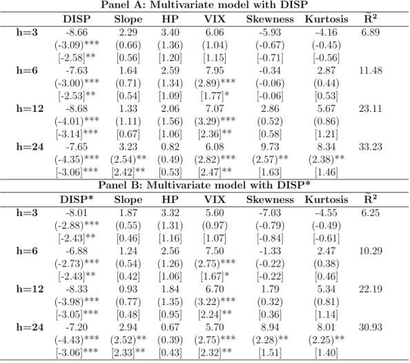
Figure 1 plots DISP along with VIX, a popular investor fear indicator capturing market forward-looking variance risk.16 _{Both series are standardized for easier comparison. While} the two series exhibit some common variation (the correlation coefficient is 29%) they tend to peak at different times. For example, unlike VIX, DISP is increasing but not very high during the 1997 Asian crisis and the 1998 Russian crisis, showing that there was no much divergence of opinions about the future aggregate stock returns during those periods. On the contrary, it exhibits several spikes during the period of the dot-com bubble, showing has very limited impact on the significance of the dispersion in options traders’ beliefs measures. The results with these additional alternative predictors are provided in the Internet Appendix.

that there were concerns about the very high stock market prices driven by the technology sector. In particular, DISP peaks in 2000:03 when NASDAQ reaches its all-time record high and the U.S. Federal Reserve increases the fed funds rate for a second time within two months, in 2000:09 when NASDAQ slightly recovers before it finally bursts, and finally in 2001:01 when the fed funds rate is cut twice within one month just before the recession period begins. DISP also peaks in 2001:09 due to the 9/11 terrorist attack, in 2005:01, possibly due to the first concerns expressed by Robert Shiller regarding the existence of a bubble in the US housing market,17 and in 2007:11 just before the beginning of the recent recession period. After the collapse of Lehman Brothers in 2008:09, it rises but not in as extreme fashion as VIX, showing that given the apparently high risk in the market, there was no extreme dispersion in options traders’ expectations. Finally, DISP substantially increases during the latest period of the European sovereign debt crisis, and takes its all-time high value in 2012:03 after the Eurogroup agreement regarding the second bailout package for Greece, following the concerns about the success of the Private Sector Involvement (PSI) program.

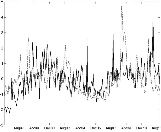
Figure 2 plots DISP and AFD, both standardized to have zero mean and variance one. While AFD is clearly smoother that DISP, it is evident that there is a remarkable similarity in the evolution of the two variables across time. More specifically, similarly to DISP, AFD is increasing during the late nineties and peaks in the period 2000:02-2000:09, just before the stock market crash. It remains relatively low in the subsequent years and increases sharply in 2007 and early 2008. Thereafter, it increases again and remains high during the whole period of the European sovereign debt crisis, taking its maximum values in the periods 2010:01-2010:05 and 2012:02-2012:03, which correspond to the two bailout agreements for Greece. Overall, Figure 2 shows clearly that DISP and AFD tend to comove across time and exhibit very similar peaks and troughs. This constitutes a first piece of evidence showing 17_{In anticipation of the publication of the second edition of Robert Shiller’s “Irrational Exuberance”, on}

January 25, 2005 CNN Money publishes a feature on the possibility of a housing bubble in the US market, accompanied by an interview of Robert Shiller expressing his concerns.

that the dispersion in trading volume across strike prices captures dispersion in expectations that appear in the options market.

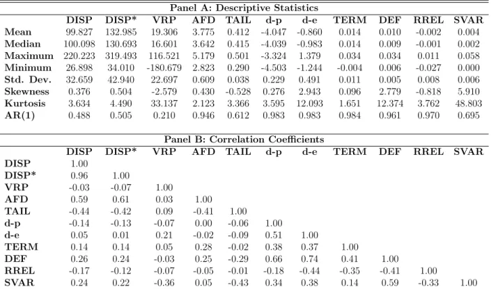
Table 1, Panel A, reports descriptive statistics about the dispersion in options traders’ expectations measures and the alternative predictive variables, while Panel B presents the respective correlation coefficients. Both dispersion in expectations measures exhibit very similar statistics, with slightly positive skewness and excess kurtosis. Unlike the majority of the alternative predictors, they are only moderately persistent with autocorrelation coef-ficients of 0.488 and 0.505 for DISP and DISP* respectively. This mitigates the problem of potentially spurious regression results caused by highly persistent regressors (see Valkanov, 2003; Torous, Valkanov, and Yan, 2004; Boudoukh, Richardson, and Whitelaw, 2008). VRP has also a low autocorrelation coefficient of 0.210 and exhibits negative skewness and very large kurtosis. In contrast, AFD has similar skewness and kurtosis to DISP and DISP* but exhibits a much higher autocorrelation coefficient of 0.946. DISP and DISP* are very highly correlated (0.96) and close to uncorrelated with VRP (-0.03 and -0.07 for DISP and DISP* respectively), showing that the dispersion in options traders’ beliefs contains different information from VRP. Moreover, they are positively and highly correlated with AFD (0.59 and 0.61 respectively), showing again that the dispersion in trading volume across strike prices embeds information similar to that of the dispersion in analysts’ forecasts. Finally, dispersion in beliefs is negatively correlated with TAIL and to a lesser extent with d-p and RREL, while showing weak positive correlation with TERM, DEF, and SVAR. The respec-tive correlations with d-e are very close to zero. Overall, both measures of dispersion in options traders’ beliefs are not highly correlated with any other variable apart from AFD, the greatest correlation occurring with TAIL.

4

In-Sample Predictability

In order to gauge the predictive power of our proposed dispersion in expectations measures, we run multiple-horizon regressions of excess stock market returns of the following form:

ret+h =αh+β

0

hzt+εt+h, (3)

where ret+h = 1200_h

[ret+1+ret+2+...+ret+h] is the annualized h-month excess return of the CRSP value-weighted index and zt is the vector of predictors. The regression analysis covers the period 1996:01-2012:12 and for each forecasting horizon we lose h observations. Under the null of no predictability the overlapping nature of the data imposes anM A(h−1) structure to the error term εt+h process. To overcome this problem we base our statistical inference on both Newey and West (1987) and Hodrick (1992) standard errors with lag length equal to the forecasting horizon. In general, the Hodrick (1992) standard errors tend to be more conservative, especially in long horizons when the null of no predictability is true (Ang and Bekaert, 2007), but have lower statistical power when the null is false (Bollerslev, Marrone, Xu and Zhou, 2014). Furthermore, to examine the robustness of the results to the Stambaugh (1999) bias, we also provide statistical inference based on empirical p-values obtained from a bootstrap simulation. The results from the bootstrap methodology are qualitatively very similar to those presented in the main body of the paper and appear in the Internet Appendix. The beta coefficients reported in the subsequent tables have been scaled and can be interpreted as the percentage annualized excess market return caused by a one standard deviation increase in each regressor.

4.1

One-month horizon predictability

Table 2, Panel A, provides the results for 1-month ahead univariate predictive regressions. The results show that the two dispersion in options traders’ expectations measures are strong predictors of stock market excess returns, as the null hypothesis of no predictability is

re-jected at the 5% level based on both Newey-West and Hodrick standard errors. The slope estimates are negative and economically significant in both cases: a one standard deviation increase in DISP predicts a negative annualized market excess return of 9.68%, while a one standard deviation increase in DISP* leads to a negative annualized market excess return of 9.20%. The adjusted R2 _{values, denoted by}

e

R2_{, are 2.23% and 1.97% for DISP and DISP*} respectively. Turning to the rest of the predictors, VRP has a positive slope (16.09), which is significant at the 1% and 5% levels based on Newey-West and Hodrick standard errors, respectively. The corresponding forecasting ratio is relatively large (7.04%). Similarly to the dispersion in options traders’ expectations, AFD has a negative coefficient (-3.77) but exhibits a negative Re2 (-0.08%) and no statistical significance. This result is in line with

Yu (2011), who shows that the predictive power of AFD is significant only at long horizons. None of the other variables is statistically significant at the 5% level (there is only marginal significance for both RREL and SVAR), a finding which is in line with Goyal and Welch’s (2008) conclusion that most of the traditional predictors have performed poorly over the last decades. Moreover, theRe2 values of most of the alternative predictors are either negative or

below 1%, similar to the findings of Goyal and Welch (2008) and Campbell and Thompson (2008). Again, the exceptions are RREL and SVAR, which still deliver lower explanatory ratios than DISP.

Next, we assess the robustness of the forecasting power of DISP and DISP* to the pres-ence of other predictive variables by conducting bivariate regressions. Panel B of Table 2 reports the results. The significance (at the 5% level) of both DISP and DISP* remains intact in all cases, showing that the information content of the dispersion in options traders’ beliefs is distinct from that of other variables that have been used in the literature. It is also interesting to note that the combination of DISP (DISP*) with VRP renders both variables strongly significant and increases the Re2 from 7.04% when considering VRP alone to 9.10%

(8.51%). Therefore, it is shown that the dispersion in options traders’ beliefs and the vari-ance risk premium are complementary measures and capture different features of investors’

expectations. Since our dispersion measures and VRP appear to be the only successful pre-dictors during our sample period, as a final robustness exercise we run trivariate predictive regressions considering combinations of DISP (or DISP*), VRP, and each of the other vari-ables. The results in Panel C of Table 2 show that the dispersion in options trading volume across strike prices and VRP continue to be significant at either the 1% or 5% level in almost all the cases.

Overall, the results in Table 2 suggest that in our sample period only the dispersion in options trading volume across strikes and VRP are consistently successful in predicting 1-month ahead excess market returns. Moreover, this predictive power is enhanced when they are combined in the same forecasting model, implying that the two measures encapsulate different pieces of information about the equity premium.

4.2

Long-horizon predictability

Table 3 provides the results for 3-, 6-, 12- and 24-month ahead univariate predictive regres-sions. Both DISP and DISP* consistently forecast negative excess market returns and are significant at either the 1% or 5% level in all but one case (the 6-month horizon with Hodrick standard errors when both DISP and DISP* are significant at the 10% level). The slope estimates continue to be economically significant, as a one standard deviation increase in DISP (DISP*) predicts a negative annualized market excess return in the range of 5.19%-7.39% (5.10%-7.10%). In terms of fit, Re2 stays between 3% and 4% for 3- and 6- month

horizons but increases substantially for longer horizons and exceeds 10% and 12% for 12-and 24-month horizons respectively. This last result is of particular importance given the relatively low persistence of the proposed dispersion in beliefs variables. The only variables that exhibit a higher Re2 at the 24-month horizon are d-p, d-e, and TERM all of which

have an autocorrelation coefficient higher than 0.98. Therefore, we conclude that DISP and DISP* can successfully capture divergence of opinions about both short and long horizon market returns.

Turning to the alternative predictors, VRP remains strongly significant for 3- and 6-month horizons with large Re2 estimates, yet its predictive power becomes less significant

for longer horizons as shown by the large decline in the explanatory ratios. This pattern is similar to Bollerslev, Tauchen and Zhou (2009), Drechsler and Yaron (2011) and Bollerslev, Marrone, Xu and Zhou (2014). More importantly, while AFD exhibits similar (albeit lower) coefficients and Re2 values than the dispersion in options traders’ beliefs measures, it does

not appear to be significant.18 This result implies that in the sample period examined, DISP and DISP* perform better than AFD not only in terms of a short 1-month horizon return predictability (which is expected given the empirical evidence provided by Yu (2011)), but also in terms of long horizon predictability. Regarding the rest of the variables, it turns out that d-p, d-e, TERM, DEF, and SVAR become significant as the horizon increases with almost monotonically increasing Re2 values. Moreover, their Newey-West t-statistics

are always considerably higher than the Hodrick t-statistics, implying that in many of these cases the significance may have arisen spuriously, due to the high persistence of the predictive variables (Ang and Bekaert, 2007).

Since the results in Table 3 suggest that only DISP, DISP*, and VRP exhibit a strong and consistent predictive pattern across all horizons, we proceed by examining trivariate predictive regressions, considering combinations of DISP (or DISP*), VRP, and each of the other variables. The results for 3-, 6-, 12- and 24-month horizons are reported in Panels A-D of Table 4. First, it can be seen that when considering a model with AFD as the third predictive variable, both DISP and DISP* remain statistically significant in most of the cases, while AFD does not exhibit any statistical significance. It is therefore confirmed once more that during the examined period the dispersion in options traders’ expectations outperforms the dispersion in analysts’ forecasts not only at short-horizon, but also at long-horizon, predictability. Turning to the rest of the trivariate models, Panels A and B show that DISP and DISP* are significant in all the cases for the 3-month horizon and in all 18_{We do, however, find significant long-horizon predictability for AFD when we examine only the common}

but one case (when dispersion in expectations and VRP are combined with RREL) for the 6-month horizon. In all the models considered, VRP continues to be strongly significant. Panels C and D show that for 12- and 24-month horizons both DISP and DISP* are again strongly significant in all the cases (based on at least one of the two alternative t-ratios), while, as in the univariate analysis, the significance of VRP for 12- and 24-month horizons weakens.

In summary, the empirical evidence regarding long-horizon predictability confirms that the dispersion in options traders’ beliefs embeds important information about long-horizon excess market returns that is not included either in the dispersion in analysts’ forecasts or in any other alternative predictor considered. Moreover, a combination of the suggested dispersion in beliefs measures with VRP can provide additional predictive power for long-horizon market returns.

5

Out-of-Sample Predictability

The results of the previous section provide clear evidence that the dispersion in options traders’ beliefs can significantly predict future excess stock market returns in-sample (IS). In this section, we evaluate the out-of-sample (OS) performance of our dispersion in beliefs measures, following Lettau and Ludvigson (2001), Goyal and Welch (2003, 2008), Guo (2006), and Campbell and Thompson (2008), among many others. The purpose of this exercise is to assess the usefulness of the dispersion in options trading volume across strike prices for an investor who has access only to real-time data when making her forecasts, and also to gauge regression parameter instability over time. Following the literature we mainly rely on OS regressions for the 1-month horizon, but for robustness purposes we also report results for 3-and 6-month horizons, keeping in mind the relatively low statistical power of OS regression analysis compared to IS analysis (Inoue and Kilian, 2004).

Zhou (2010), Ferreira and Santa-Clara (2011) and Neely, Rapach, Tu and Zhou (2014), we estimate the model in equation (3) recursively using the first s=s0, ..., T −h observations, withT being the total number of months in our sample period andhthe forecasting horizon. Next, based on the estimated parameters, we form for each time period s the OS forecasts for the expected excess market return using the concurrent values of the predictor variables:

b

res+h =αbs+βb

0

szs. (4)

The initial estimation period is 1996:01-1999:12 and the first prediction is made for 2000:01. This way we create a series of TOS OS forecasts that is compared to a series of recursively estimated historical averages, which correspond to OS forecasts of a restricted model with only a constant as a regressor. We employ four measures to assess the OS predictability performance of our dispersion in expectations measures.

The first measure is the OS R2_{, denoted byR}2

OS, which takes the form:

R2_OS = 1− M SEU M SER , (5) where M SEU = _T1 OS PT−h s=s0(res+h−rebs+h) 2

is the mean square error of the unrestricted model and M SER = _T1

OS

PT−h

s=s0(res+h−rees+h)

2

is the mean square error of the restricted model, withre_es+h being the recursively estimated historical average. R2OS takes positive val-ues whenever the unrestricted model outperforms the restricted model in terms of predictive power (i.e. M SEU < M SER).

The second measure of OS performance is the MSE-F test from McCracken (2007):

M SE−F = (TOS−h+ 1)

M SER−M SEU M SEU

, (6)

which tests the null hypothesis that the restricted model’s MSE is less than or equal to the unrestricted model’s MSE. McCracken (2007) shows that the F-statistic follows a

non-standard normal distribution and provides appropriate critical values using Monte Carlo simulations.

The third OS performance measure is the MSE-Adjusted test of Clark and West (2007). It tests the null hypothesis thatM SERis less than or equal toM SEU, against the alternative hypothesis thatM SERis greater thanM SEU. In addition, it adjusts for the fact that under the null hypothesis the unrestricted model’s forecasts are contaminated by noise caused by estimating coefficients with zero population values. To this end, Clark and West (2007) define: b fs+h = (res+h−rees+h) 2 − (res+h−rebs+h) 2 −(re_es+h−rebs+h) 2 , (7)

and postulate that by regressing on a constant and calculating the respective t-statistic it is possible to test the (one-sided) null hypothesis using standard normal critical values.19,20

The final measure of OS forecasting performance is the constrained OS R2 _{(denoted by} R2

COS) suggested by Campbell and Thompson (2008). This measure is the same asR2OSapart from the fact that it sets the OS forecasts of the unrestricted model equal to zero whenever they take negative values. Therefore, an investor’s real time equity premium prediction becomes in accordance with standard asset pricing theory.

Table 5 presents the results for 1-, 3- and 6-month horizon OS predictability. In the case of the 1-month horizon, DISP and DISP* exhibit positiveR2

OS estimates of 1.70% and 1.55% respectively, signifying that they generate MSEs that are lower than the restricted model’s MSE. Moreover, this outperformance of the unrestricted models based on the dispersion in options traders’ expectations is statistically significant, as shown by the F and MSE-Adjusted statistics. When we impose the restriction of positive expected equity premium the fit is improved for both dispersion in beliefs measures, with R2_COS becoming 2.16% for 19_{To control for the autocorrelation in forecast errors when examining long-horizon OS predictability, the}

t-statistics are calculated using Newey and West (1987) standard errors.

20_{In addition, we have also considered the ENC-NEW encompassing test of Clark and McCracken (2001).}

The results are provided in the Internet Appendix and are similar (and even stronger) than the results of the MSE-F and MSE-Adjusted tests.

DISP and 2.44% for DISP*. Turning to the remainder of the predictors, only VRP provides a positive R2

OS, of 7.96%, with the MSE-F and MSE-Adjusted tests strongly rejecting the respective null hypotheses. AFD delivers a lower MSE than the historical average only when the Campbell and Thompson (2008) restriction is imposed, but still its R2

COS is lower than the corresponding estimates of both DISP and DISP*. Since univariate analysis suggests that only the dispersion in options trading volume across strikes and VRP have significant OS forecasting performance, we proceed by combining the two dispersion in options traders’ beliefs measures with VRP. The results show that the bivariate models increase the R2_OS, which becomes 9.06% in the regression including DISP and VRP, and 8.56% in the case of DISP* and VRP. It is therefore confirmed that the information content of the dispersion in options traders’ expectations is different from that of VRP. Moreover, the MSE-F and MSE-Adjusted tests reject the respective null hypotheses even more decisively than in the univariate regressions.

The results for the 3-month horizon are similar to those for the 1-month horizon but stronger for both dispersion in beliefs measures and the VRP. This is in line with the IS regression results presented in the previous section. In particular, DISP (DISP*) has an R2

OS of 3.37% (3.04%) while VRP produces an estimate of 12.47%. The F and MSE-Adjusted tests provide even stronger evidence against the respective null hypotheses than at the 1-month horizon. As in the 1-month horizon analysis, apart from DISP, DISP* and VRP, none of the other predictors exhibit positiveR2

OSestimates. Furthermore, the bivariate model including the dispersion in options traders’ expectations and VRP is even more successful in terms of OS return predictability than at the 1-month horizon. The results for the 6-month horizon are in the same vein with the evidence from the other horizons. In particular, the R2

OS values of DISP and DISP* remain positive while the MSE-F and MSE-Adjusted tests still reject the respective null hypotheses at either the 5% or 10% level. Moreover, except for VRP none of the other alternative predictors provides a positive R2

OS, while the combination of DISP (or DISP*) with VRP offers even stronger OS predictability than at

the other horizons.

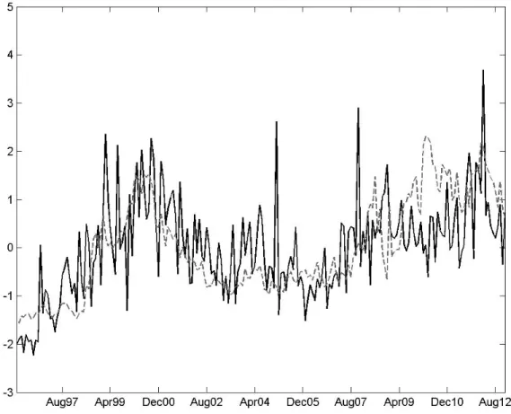
Following Goyal and Welch (2008), Rapach, Strauss and Zhou (2010) and Huang, Jiang, Tu and Zhou (2015), we also provide in Figure 3 time-series graphs of the differences in the 1-month horizon cumulative square prediction error between the restricted model and each of the unrestricted models. These graphs depict the OS performance of the unrestricted models compared to the restricted model across time. More specifically, whenever the line in each of the graphs increases, the unrestricted model outperforms the historical average model, while the opposite holds whenever the line decreases. We examine the OS performance using both the original unrestricted model predictions (solid black lines) and the predictions after imposing the restriction of positive forecasted equity premium (dashed grey lines). Figure 3 shows that the DISP and DISP* models outperform the historical average model during most of the period examined, exhibiting a lower performance only at the latest part of the sample. VRP, on the other hand, slightly outperforms the historical average model for most of the sample period but performs substantially better after the financial crisis. From the rest of the variables, only AFD and d-p provide some consistent outperformance over the historical average during specific periods, but they end up having a higher overall cumulative prediction error than the restricted model. The conclusions when we impose the positive equity premium restriction are practically the same; DISP, DISP*, VRP and now also AFD have consistently positive slopes but AFD exhibits the lowest difference in the cumulative prediction error.

Overall, the empirical evidence regarding OS return predictability suggests that only the dispersion in options traders’ expectations and VRP can consistently beat the historical av-erage and their predictive power is enhanced when they are combined in one bivariate model. On the other hand, the dispersion in analysts’ forecasts outperforms the historical average only when the Campbell and Thompson (2008) restriction is imposed, yet its performance is still inferior to that of the dispersion in options traders’ expectations.

6

Economic Significance

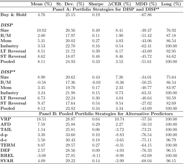
In this section, we evaluate the economic significance of the information embedded in the dis-persion in options traders’ beliefs in terms of forecasting stock returns. To this end, following Goyal and Santa-Clara (2003), Campbell and Thompson (2008), Ferreira and Santa-Clara (2011), Maio (2013, 2014), Rapach, Strauss, Tu and Zhou (2011) and Huang, Jiang, Tu and Zhou (2015), we create market-timing and portfolio rotation strategies that rely on the OS forecasting power of the suggested dispersion in expectations measures and the alternative predictors.

6.1

Market-timing strategies

We assess the economic significance of the dispersion in options traders’ beliefs predictability by creating an active trading strategy that is based on its OS predictive power for 1-month ahead stock market excess returns. To this end, we assume a mean-variance investor who allocates her wealth every month between the market portfolio and the risk-free asset based on forecasts of the equity premium and the variance of market returns. More specifically, at the end of each month s, the investor forms an estimate of the excess market return21 using the procedure described in the previous section and an estimate of the market return variance using all available data up to times. In this setting, the portfolio weight attributed to the stock market index takes the form:

ωs= b res+1 γ_bσ2

s+1

, (8)

where re_bs+1 is the OS forecast of the 1-month ahead excess stock market return, γ is the risk aversion coefficient, which is set equal to three, andσ_b2

s+1 is the estimate of the variance of the stock market return. Following Campbell and Thompson (2008), we impose realistic leverage values by constraining the portfolio weight on the market indexωs to lie between 0

and 1.5.

Alternatively, we assume that the investor follows a binary rule for selecting her portfolio weights. In particular, we consider two scenarios: one where short-sales are not allowed and one where short-sales are allowed. In the first scenario we have:

ωs = 1 if rebs+1 ≥0

ωs = 0 if rebs+1 <0, (9)

while in the second scenario we have:

ωs = 1.5 if rebs+1 ≥0

ωs = −0.5 if rebs+1 <0. (10)

The realized return from each of the active trading strategies presented above can be represented by:

Rp,s+1 =ωsRm,s+1+ (1−ωs)Rf,s+1, (11) whereRm,s+1 denotes the simple market return andRf,s+1 denotes the return of the riskless asset. Therefore, iterating this procedure forward, we create a series of realized portfolio returns based on the OS forecasting power of each forecasting variable and we compare each strategy with a buy-hold strategy. When leverage is allowed this passive strategy allocates 150% of the wealth to the market index and -50% to the risk-free asset. When leverage is not allowed this strategy consistently allocates 100% of the wealth to the market index.

For each trading strategy, we estimate the mean portfolio return, the standard deviation, and its Sharpe ratio. Moreover, since the Sharpe ratio weights equally the mean and volatility of the portfolio returns, we follow Campbell and Thompson (2008), Ferreira and Santa-Clara (2011), and Maio (2014) and compute a certainty equivalent return (∆CER) in excess of the

buy-hold strategy: ∆CER =E(Rp,s+1)−E R¯p,s+1 +γ 2 V ar R¯p,s+1 −V ar(Rp,s+1) , (12)

where γ is the risk aversion coefficient, Rp,t+1 is the portfolio return of the market-timing strategy and ¯Rp,t+1 is the portfolio return of the buy-hold strategy. ∆CER essentially repre-sents the change in the investor’s utility resulting from her choice to follow the active instead of the passive trading strategy. It can also be interpreted as the annual “fee”that an investor is willing to pay to invest in the active strategy instead of investing in the passive strategy. As an additional performance measure, we also estimate the maximum drawdown (MDD), which represents the maximum loss than an investor can incur if she enters the strategy at any time during its implementation period. All measures apart from the MDD are in annualized terms. Finally, we also report the percentage of months that each active strategy takes a long position on the stock market index.

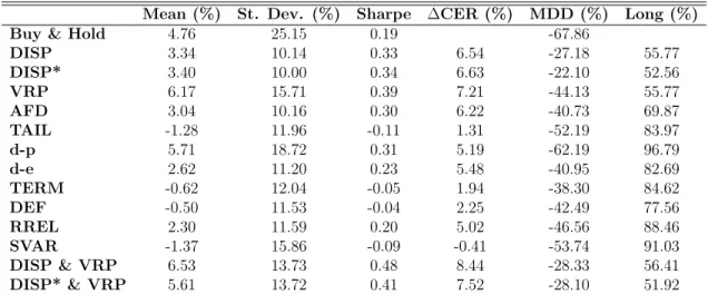
The performance results from the strategies with the mean-variance weights are presented in Table 6. The strategy associated with DISP exhibits an annualized Sharpe ratio of 0.33, while the one associated with DISP* has a Sharpe ratio of 0.34. Both Sharpe ratios are substantially higher than the one associated with the buy-hold strategy (0.19), a result which mainly stems from the remarkably low volatilities that the two dispersion in options traders’ beliefs measures exhibit (10.14% for DISP and 10.00% for DISP* respectively). Furthermore, the ∆CER of the strategy based on DISP is 6.54% per year and that of the strategy based on DISP* is 6.63%, thus showing that the utility provided by the active strategies related to the dispersion in beliefs is significantly higher than the utility of the buy-hold strategy. More importantly, DISP and DISP* outperform all other alternative predictors apart from VRP, which performs slightly better, exhibiting a Sharpe ratio of 0.39 and a ∆CER of 7.21%. On the other hand, while the strategy based on AFD also outperforms the buy-hold strategy, its performance is marginally inferior to the DISP and DISP* strategies (Sharpe ratio of

0.30 and ∆CER of 6.22%). This result indicates again that while the dispersion in options traders’ beliefs and the dispersion in analysts’ forecasts share some common information, the former can provide higher economic gains when used as a predictive variable for future stock market returns. It is also important to note that both DISP and DISP* exhibit by far the lowest MDDs (-27.18% and -22.10% respectively), showing that the dispersion in options traders’ beliefs can be used as a warning signal in turbulent periods and severely limits an investor’s potential cumulative loss. Finally, when we combine either DISP or DISP* in bivariate models with VRP, the performance of the respective trading strategies improves in comparison to the strategy based solely on VRP. Specifically, the strategy containing VRP and DISP (DISP*) produces a Sharpe ratio of 0.48 (0.41) and a ∆CER of 8.44% (7.52%) per year, thus confirming that the dispersion in options traders’ beliefs is beneficial in economic terms for an investor who already uses the VRP for her investment decisions.

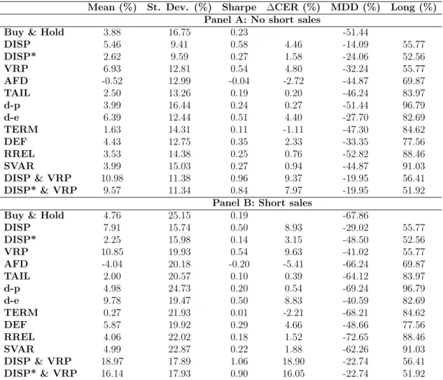
The results from the strategies with the alternative binary weights are reported in Table 7. When short sales are not allowed (Panel A), both DISP and DISP* outperform the buy-hold strategy in terms of Sharpe ratio (0.58 and 0.27 respectively compared to 0.23) and exhibit positive ∆CERs (4.46% and 1.58% respectively). Moreover, DISP outperforms all variables except for VRP, while DISP* outperforms all variables apart from VRP, d-e and DEF. However, a combination of either DISP or DISP* with VRP yields substantially higher performance compared to the strategy based only on VRP. In particular, the Sharpe ratio (∆CER) of the bivariate model with DISP and VRP becomes 0.96 (9.37%) and that of DISP* with VRP becomes 0.84 (7.97%) compared to only 0.54 (4.80%) when VRP is considered alone.22 Furthermore, similarly to the mean-variance weights, both DISP and DISP* exhibit the lowest MDDs among all variables considered (-14.09% and -26.06% respectively). Finally, when using binary weights the performance of AFD remarkably deteriorates, resulting in a negative Sharpe ratio and negative ∆CER (-0.04 and -2.72% respectively). The pattern in the performance of the different trading strategies is very similar when short-sales are allowed 22_{In contrast, unreported results show that the combination of d-e (DEF) with VRP offers a Sharpe ratio}

(Panel B). The main differences are that DISP* underperforms the buy-hold strategy in terms of Sharpe ratio (but still exhibits a positive ∆CER (3.15%)) and that its MDD is relatively increased to -48.50%. These differences are due to the fact that extreme realizations (highly positive and highly negative market returns) now have a larger impact on the portfolio returns. However, all the other results are in accordance with the evidence provided for the case of prohibited short sales.

In summary, the empirical evidence associated with the market-timing strategies shows that the OS forecasting ability of the dispersion in options’ traders beliefs for future mar-ket returns is economically significant, especially for an investor who already considers the information from VRP for her investment decisions. Moreover, in all cases examined the dispersion in options’ traders beliefs outperforms the dispersion in analysts’ forecasts and most of the other predictors.

6.2

Portfolio rotation strategies