Mining association rules with multiple minimum supports: a new
mining algorithm and a support tuning mechanism
Ya-Han Hu
a, Yen-Liang Chen
b,*
aDepartment of Information Management, National Central University, Chung-Li 320, Taiwan, ROC bDepartment of Information Management, National Central University, Chung-Li 320, Taiwan, ROC Received 15 June 2003; received in revised form 2 September 2004; accepted 8 September 2004
Available online 30 November 2004
Abstract
Mining association rules with multiple minimum supports is an important generalization of the association-rule-mining problem, which was recently proposed by Liu et al. Instead of setting a single minimum support threshold for all items, they allow users to specify multiple minimum supports to reflect the natures of the items, and an Apriori-based algorithm, named MSapriori, is developed to mine all frequent itemsets. In this paper, we study the same problem but with two additional improvements. First, we propose a FP-tree-like structure, MIS-tree, to store the crucial information about frequent patterns. Accordingly, an efficient MIS-tree-based algorithm, called the CFP-growth algorithm, is developed for mining all frequent itemsets. Second, since each item can have its own minimum support, it is very difficult for users to set the appropriate thresholds for all items at a time. In practice, users need to tune items’ supports and run the mining algorithm repeatedly until a satisfactory end is reached. To speed up this time-consuming tuning process, an efficient algorithm which can maintain the MIS-tree structure without rescanning database is proposed. Experiments on both synthetic and real-life datasets show that our algorithms are much more efficient and scalable than the previous algorithm.
D2004 Elsevier B.V. All rights reserved.
Keywords:Data mining; Association rules; Minimum supports; FP-tree
1. Introduction
Data mining has recently attracted considerable attention from database practitioners and researchers because of its applicability in many areas such as decision support, market strategy and financial
fore-casts. Many approaches have been proposed to find out useful and invaluable information from huge databases[2,7]. One of the most important approaches is mining association rules, which was first introduced in Ref.[1]and can be stated as follows.
LetI={i1,i2,. . .,im} be a set of items andD be a set of transactions, where each transaction T (a data case) is a set of items so thatTpI. An association rule is an implication of the form,XYY, whereXoI,YoI
and X\Y=f. The ruleXYY holds in the transaction 0167-9236/$ - see front matterD2004 Elsevier B.V. All rights reserved.
doi:10.1016/j.dss.2004.09.007
* Corresponding author. Tel.: +886 3 4267266; fax: +886 3 4254604.
E-mail address:[email protected] (Y.-L. Chen).
setTwith confidencec, ifc% of transactions inTthat supportXalso supportY. The rule hassupport sinTif
s% of the transactions inTcontainsX[Y. Given a set of transactions D (the database), the problem of mining association rules is to discover all association rules that have support and confidence greater than the user-specified minimum support (calledminsup) and minimum confidence (calledminconf).
The key element that makes association-rule mining practical is minsup. It is used to prune the search space and to limit the number of rules generated. However, using only a single minsup
implicitly assumes that all items in the database are of the same nature or of similar frequencies in the database. This is often not the case in real-life applications [10,14]. In the retailing business, cus-tomers buy some items very frequently but other items very rarely. Usually, the necessities, consumables and low-price products are bought frequently, while the luxury goods, electric appliance and high-price products infrequently. In such a situation, if we set
minsup too high, all the discovered patterns are concerned with those low-price products, which only contribute a small portion of the profit to the business. On the other hand, if we setminsup too low, we will generate too many meaningless frequent patterns and they will overload the decision makers, who may find it difficult to understand the patterns generated by data mining algorithms.
The same difficulty may occur when we are about to mine medical records. Mining medical records is a very important issue in real-life application and it can reveal which symptoms are related to which disease. However, many important symptoms and diseases are infrequent in medical records. For example, flu occurs much more frequent than severe acute respiratory syndrome (SARS), and both have symptoms of fever and persistent cough. If the value of minsup is set high, though the rule bfluYfever, coughQ can be found, we would never find the rule bSARSYfever,
cough.Q To find this SARS rule, we need to set the value of minsup very low. However, this will cause lots of meaningless rules to be found at the same time. The dilemma faced in the two applications above is called the rare item problem [11]. In view of this, researchers either (A) split the data into a few blocks according to the frequencies of the items and then mine association rules in each block with a differentminsup
[9], or (B) group a number of related rare items together into an abstract item so that this abstract item is more frequent [6,9]. The first approach is not satisfactory because rules that involve items across different blocks are difficult to find. Similarly, the second approach is unable to find rules that involve individual rare items and the more frequent items. Clearly, both approaches are ad hoc andbapproximateQ[9].
To solve this problem, Liu et al.[10]have extended the existing association rule model to allow the user to specify multiple minimum supports to reflect different natures and frequencies of items. Specifically, the user can specify a different minimum item support for each item. Thus, different rules may need to satisfy different minimum supports depending on what items are in the rules. This new model enables users to produce rare item rules without causing frequent items to generate too many meaningless rules. However, the proposed algorithm in Liu et al. [10], named the MSapriori algorithm, adopts an Apriori-like candidate set gen-eration-and-test approach and it is always costly and time-consuming, especially when there exist long patterns. In this study, we propose a novel multiple item support tree (MIS-tree for short) structure, which extends the FP-tree structure[8]for storing compressed and crucial information about frequent patterns, and we develop an efficient MIS-tree-based mining method, the CFP-growth algorithm, for mining the complete set of frequent patterns with multiple minimum supports. The experimental result shows that the CFP-growth algorithm is efficient and scalable on both synthetic data and real-life data, and that it is about an order of magnitude faster than the MSapriori algorithm.
In real-life applications, users cannot find appli-cable support value at once and always tune its support value constantly. To do this, every time when users change the items’ minsup, they must rescan database and then execute the mining algorithm once again. It is very time-consuming and costly. Thus, it is attractive to consider the possibility of designing a maintenance algorithm for tuning minimum supports (MS for short). In the past, although there were few researches dealing with this problem[3]for single MS scenario, most of previous researches are concerned with how to maintain the knowledge in correctness after the database is updated[4,5,12,13].
The problem addressed above will become even more serious for frequent pattern mining with multiple
MS, because previously users only need to tune a single MS threshold but now they need to tune many MS thresholds. Thus, it is even more demanding to have a maintenance algorithm for MS tuning. This paper proposes, therefore, a maintenance algorithm to keep our MIS-tree in correct status after tuning MS. The experimental evaluation shows that our MIS-tree maintenance method can react almost instantaneously when tuning MS.
The remaining of the paper is organized as follows. In Section 2, we briefly review the Apriori algorithm [1], the MSapriori algorithm [10] and the FP-growth algorithm[8]. Some of those concepts will be used in developing our algorithm. Section 3
introduces the MIS-tree structure and its construction method. Then, we develop a MIS-tree-based frequent pattern mining algorithm, the CFP-growth algorithm, in Section 4. In Section 5, we propose the main-tenance algorithm for MS tuning. The performance
evaluation is done in Section 6. Finally, the
con-clusion is drawn inSection 7.
2. Related work
In the section, three algorithms, including the Apriori algorithm, the MSapriori algorithm and the FP-growth algorithms, are briefly reviewed. The Apriori algorithm is the most popular algorithm for mining frequent itemsets. However, it has two problems: (1) it only allows a single MS threshold, and (2) its efficiency is usually not satisfactory. As to the first problem, the MSapriori algorithm extends the Apriori algorithm so that it can find frequent patterns with multiple MS thresholds. As for the second problem, many algorithms have been proposed to improve the efficiency. The FP-growth algorithm is one of these improved algorithms and is probably the most well-known. The FP-growth algorithm contains two phases, where the first phase constructs an tree, and the second phase recursively projects the FP-tree and outputs all frequent patterns. In the following, we review them in order.
2.1. The Apriori algorithm
The Apriori algorithm[1]discovers frequent item-sets from databases by iteration. Basically, iterationi
computes the set of frequent i-itemsets (frequent patterns with i items.) In the first iteration, the set of candidate 1-itemsets contains all items in the database. Then, the algorithm counts their supports by scanning the database, and those 1-itemsets whose supports satisfy the MS threshold are selected as frequent 1-itemsets.
In thekth (kz2) iteration, the algorithm consists of
two steps. First, the set of frequent itemsetsLk1found in the (k1)th iteration is used to generate the set of candidate itemsetsCk. Next, we compute the supports of candidate itemsets in Ck by scanning the database and then we obtain the setLkof frequentk-itemsets.
The iteration will be repeatedly executed until no candidate patterns can be found.
2.2. The MSapriori algorithm
The MSapriori algorithm [10] can find rare item rules without producing a huge number of mean-ingless rules. In this model, the definition of the minimum support is changed. Each item in the database can have its minsup, which is expressed in terms ofminimum item support(MIS). In other words, users can specify different MIS values for different items. By assigning different MIS values to different items, we can reflect the natures of the items and their varied frequencies in the database.
Definition 1.LetI={a1,a2,. . .,am} be a set of items and MIS(ai) denote the MIS value of item ai. Then the MIS value of itemsetA={a1,a2,. . .,ak} (1VkVm) is equal to:
min MIS½ ð Þa1 ; MISð Þa2 ;. . .; MISð Þak
Example 1. Consider the following items in a
database,bread,shoesandclothes. The user-specified MIS values are as follows:
MISðbreadÞ ¼2%; MISðshoesÞ ¼0:1%;
MISðclothesÞ ¼0:2%
If the support of itemset{clothes,bread} is 0.15%, then itemset{clothes,bread} is infrequent because the MIS value of itemset{clothes, bread} is equal to min[MIS(clothes), MIS(bread)]=0.2%, which is larger than 0.15%.
The task of mining association rules is usually decomposed into two steps:
(1) Frequent itemset generation: to find all frequent itemsets with supports exceedingminsup. (2) Rule generation: to construct from the set of
frequent itemsets all association rules with confidences exceeding the minimum confidence. Note that, in order to generate the association rules from a frequent itemset, not only we need to know the support of this itemset, but the supports of all its subsets must also be known. Otherwise, it would be impossible to compute the confidences of all related rules.
When there is only one single MS, the above two steps satisfy thedownward closure property. That is, if an itemset is frequent, then all its subsets are also frequent. Therefore, after applying the Apriori algo-rithm we can find the support values of all subsets of frequent itemset{A, B, C, D} and all related rules as well. On the contrary, when there are multiple MS, the downward closure property no longer holds. That is, some subsets of a frequent itemset may not be frequent and their supports will be missing.
Example 2.Consider four items A, B, C and D in a
database. Their MIS values are:
If the support of itemset{B, C} is 13% and that of itemset{B, D} is 14%, then both itemsets {B, C} and {B, D} are infrequent; for they do not satisfy their MIS values (MIS(B, C)=min[MIS(B), MIS(C)]=15% and MIS(B, D)=min[MIS(B), MIS(D)]=15%). Sup-pose the support of itemset{A, B, C, D} is 8%. Then itemset{A, B, C, D} is frequent because MIS(A) is only 5%.
The above example indicates that a subset of a frequent itemset may be not frequent. Thus, the fact that the support of a frequent itemset is known does not necessarily imply that the supports of all its subsets are known. As a result, knowing the supports of all frequent itemsets is not enough to generate association rules.
The MSapriori algorithm aims to find all frequent itemsets by modifying the well-known Apriori
algo-rithm. These modifications include presorting all the items according to their MIS values and modifying the candidate set generation procedure. After the applica-tion of the MSapriori algorithm, all frequent itemsets are found but the supports of some subsets may be still unknown. Thus, if we intend to generate association rules, we need a post-processing phase to find the supports of all subsets of frequent itemsets. This procedure is time-consuming because we need to scan the database again and compute the supports of all subsets of frequent itemsets.
2.3. The FP-growth algorithm
An FP-tree is an extended prefix-tree structure for storing compressed and crucial information about frequent patterns, while the FP-growth algorithm uses the FP-tree structure to find the complete set of frequent patterns[8].
An FP-tree consists of one root labeled as bnullQ, a set of item prefix subtrees as the children of the root and a frequent-item header table. Each node in the prefix subtree consists of three fields:item-name,
count andnode-link. Thecount of a node records the number of transactions in the database that share the prefix represented by the node, and node-link links to the next node in the FP-tree carrying the same
item-name. Each entry in the frequent-item header table consists of two fields: item-name and head of node-link, which points to the first node in the FP-tree carrying the item-name. Besides, the FP-FP-tree assumes that the items are sorted in decreasing order of their support counts, and only frequent items are included.
After the FP-tree is built, the FP-growth algorithm recursively builds conditional pattern base and
conditional FP-tree for each frequent item from the FP-tree and then uses them to generate all frequent itemsets.
3. Multiple Item Support tree (MIS-tree): design and construction
In this section, a new tree structure, named the MIS-tree, is proposed for mining frequent pattern with multiple MS. It is an extended version of the FP-tree structure.
MIS(A)=5% MIS(B)=15%
According to Definition 1, letDB={T1,T2,. . .,Tn} be a transaction database, where Tj (ja[1. . .n]) is a transaction containing a set of items inI. The support of an itemset A is the percentage of transactions containingA inDB. If itemset A’s support is no less than MIS(A), then patternA is a frequent pattern.
LetMINdenote the smallest MIS value of all items (MIN=min[MIS(a1), MIS(a2),. . ., MIS(am)]), and let the set of MIN_frequent items F denote the set of those items with supports no less thanMIN.
Example 3.In Example 2, we have four items as well
as their MIS values. The value of MIN is equal to
min[MIS(A), MIS(B), MIS(C), MIS(D)]=5%. If A.support=3%, B.support=20%, C.support=25%, D.support=50%, then the set of MIN_frequent items
F={B, C, D} Fig. 1. MIS-tree construction algorithm.
Table 1
A transaction database DB
TID Item bought Item bought (ordered)
100 d, c, a, f a, c, d, f
200 g, c, a, f, e a, c, e, f, g 300 b, a, c, f, h a, b, c, f, h
400 g, b, f b, f, g
Lemma 1. Let Lk be the set of frequent k-itemsets.
Then each item in Lk(kN1) must be in F.
There is a very important difference between the FP-tree and the MIS-tree: the FP-tree only contains frequent items, but the MIS-tree consists of not only all frequent items but also those infrequent items with supports no less thanMIN. Based on Lemma 1, each item in Lk must belong to F. We must retain those infrequent items which belong to F because their supersets may be frequent itemsets.
Example 4. In Example 3, we know that A.
sup-port=3%, B.support=20%, C.support=25%, D. sup-port=50%, and the set of MIN_frequent itemsF={B, C, D}. Consider the infrequent item C, where the support of item C=25% and MIS(C)=30%. We must retain the infrequent item C because the itemset{B, C} may be frequent. However, if the support of infre-quent item C is less thanMIN (not belonging toF), we can discard item C immediately.
Definition 2(MIS-tree). A multiple item support tree
is a tree structure defined as follows.
(1) It consists of one root labeled asbnullQ, a set of item prefix subtrees as the children of the root,
and a MIN_frequent item header table which contains all items inF.
(2) Each node in the item prefix subtree consists of three fields: item-name, count and node-link, where item-name registers which item this node presents, count registers the number of transactions represented by the portion of the path reaching this node, and node-link
links to the next node in the MIS-tree carrying the same item-name, or null if there is none.
(3) Each entry in the MIN_frequent item header table consists of three fields:item-name, item’s minsup MIS(ai) and head of node-link which points to the first node in the MIS-tree carrying the item-name.
(4) All the items in the table are sorted in non-increasing order in terms of their MIS values.
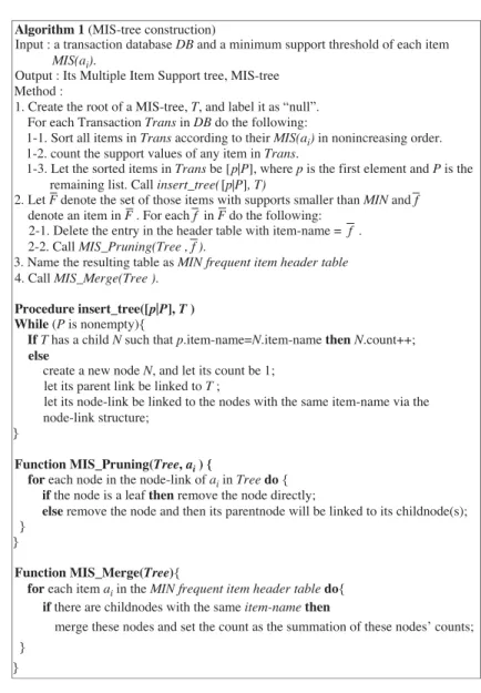
According to Definition 2, we have the following MIS-tree construction algorithm and each function used in Algorithm 1 is shown in Fig. 1.
We use the following example to illustrate the MIS-tree construction process.
Table 2
The MIS value of each item in DB
Item a b c d e f g h
MIS value 4 (80%) 4 (80%) 4 (80%) 3 (60%) 3 (60%) 2 (40%) 2 (40%) 2 (40%)
Example 5 (The construction of MIS-tree). Let us consider the transaction database DB shown inTable 1. The MIS value of each item is shown in Table 2. According to Algorithm 1, the order of the items in the MIS-tree is arranged according to their MIS values in non-increasing order. For ease of discussion, the
rightmost column ofTable 1lists all the items in each transaction following this order.
To create the MIS-tree, we first create the root of the tree, labeled as bnullQ. The scan of the first transaction leads to the construction of the first branch
of the MIS-tree: ((a:1), (c:1), (d:1), (f:1)). Notice that all items in the transaction would be inserted into the tree according to their MIS values in non-increasing order. The second transaction (a, c, e, f, g) shares the same prefix (a, c) with the existing path (a, c, d, f). So, the count of each node along the prefix is increased by 1 and the remaining item list (e, f, g) in the second transaction would be created as the new nodes. The new node (e:1) is linked as a child of (c:2); node (f:1) as a child of (e:1); node (g:1) as a child of (f:1). For the third transaction (a, b, c, f, h), it shares only the node (a). Thus, a’s count is increased by 1, and the remaining item list (b, c, f, h) in the third transaction would be created just like the second transaction. The remaining transactions in DB can be done in the same way.
To facilitate tree traversal, a MIN_frequent item header table is built in which each item points to its occurrences in the tree via the head of node-link. Nodes with the same item-name are linked in sequence via such node-links. After all the trans-actions are scanned, the tree with the associated node-links is shown in Fig. 2.
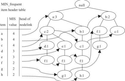
After scanning all the transactions, we will get the count of each item as (a:3, b:3, c:4, d:1, e:1, f:4, g:2, h:1) and the initial MIS-tree shown in Fig. 2. According to Lemma 1, we only need to retain those items with supports no less thanMIN=2 (all items in
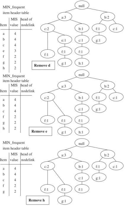
F) in our MIS-tree. So, we remove the nodes with item-name=(d, e, h) and the result is shown inFig. 3. After these nodes are removed, the remaining nodes in the MIS-tree may contain child nodes Fig. 4. MIS_Merge process of MIS-tree.
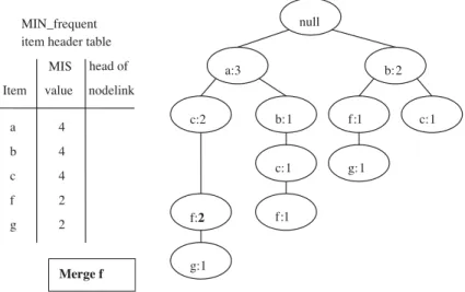
carrying the same item-name. For the sake of compactness, we traverse the MIS-tree and find that node (c:2) has two child nodes carrying the same item-name f. We merge these two nodes into a single node with item-name=f, and its count is set as the sum of counts of these two nodes (shown in Fig. 4). At last, the complete and compact MIS-tree is shown in
Fig. 5.
To construct the MIS-tree, our algorithm only needs one scan of the transaction database. This scan happens when we insert every transaction into the tree. After insertion, we delete those superfluous items from MIS-tree and merge nodes for compactness. Next, we will show that the MIS-tree contains the complete information for frequent pattern mining with multiple MS.
Lemma 2. Given a transaction database DB and a
support threshold MIS(ai) of each item ai, the
constructed MIS-tree contains the complete informa-tion about frequent patterns in DB.
Rationale: In the MIS-tree’s construction process, each transaction inDB is mapped to one path in the MIS-tree. And all MIN_frequent items information in each transaction is completely stored in the MIS-tree. Notice that we retained those infrequent items with supports no less than MIN in our MIS-tree because Lemma 1 indicates that these items’ supersets may be frequent.
4. The CFP-growth algorithm
In this section, we will propose the CFP-growth method for mining the complete set of frequent patterns. Before presenting the algorithm, we observe some interesting properties of the MIS-tree structure.
Definition 3 (Conditional pattern). A pattern x is
calledai’s conditional pattern ifaiis inxand satisfies MIS(x)=MIS(ai).
Example 6.In Example 2, itemset{A, B, C, D} is an
A’s conditional pattern because MIS(A)=MIS({A, B, C, D}).
Definition 4 (Conditional frequent pattern). A
fre-quent pattern x is called ai’s conditional frequent pattern ifai is inxand satisfies MIS(x)=MIS(ai).
Example 7.In Example 2, itemset{A, B, C, D} is an
A’s conditional frequent pattern because itemset{A, B, C, D} is frequent and MIS(A)=MIS({A, B, C, D}).
Property 1 (Node-link property). For any frequent
item ai, all the possible ai’s conditional frequent patternscan be obtained by followingai’snode-link, starting fromai’s head in the MIS-tree header.
This property is directly based on the construction process of the MIS-tree. Through the ai’s node-link, all the transactions (built in the MIS-tree) related toai would be traversed. Hence, it will find all the pattern information related to ai by followingai’snode-link, and then all theai’sconditional frequent patternscan be obtained.
Property 2 (Prefix path property). To calculate the
ai’sconditional frequent patternsin a pathP, only the prefix subpath of node ai in P needs to be accu-mulated, and the frequency count of every node in the prefix path should carry the same count as nodeai.
Rationale: Let the nodes along the path P be labeled asa1,a2,. . .,anin such an order thata1is the root of the prefix subtree,anis the leaf of the subtree in P, and ai (1ViVn) is the node being referenced. Based on the process of constructing MIS-tree presented in Algorithm 1, for each prefix node
ak(1Vkbi), the prefix subpath of the node ai in P occurs together withakexactlyai.counttimes. Thus, every such prefix node should carry the same count as nodeai. Notice that a postfix nodeam(ibmVn) along the same path also co-occurs with nodeai. However, the patterns with am will be generated at the examination of the postfix node am, and enclosing them here will lead to redundant generation of the patterns that would have been generated foram.
The MIS-tree itself does not give the frequent itemsets directly. Nevertheless, the CFP-growth algo-rithm recursively buildsbconditional MIS-treesQ, from the MIS-tree, which results in the set of all frequent itemsets. Let us illustrate the procedure by an example.
Example 8.According to Property 1, we collect all the
patterns that a nodeaiparticipates in by starting from
ai’s head (in the MIN_frequent header table) and followingai’s node-link. We examine the CFP-growth algorithm by starting from the bottom of the header table.
For the MIS-tree inFig. 5, let us consider how to build a conditional pattern base and conditional MIS-tree for item g. First, the node-link of item g is followed. Each such path in the MIS-tree ends at a nodebgQ. However, we exclude the nodebgQitself and add it to the conditional pattern base and the condi-tional MIS-tree for item g. Counter of each node in the path is set to that of the node bgQ itself. In this example, following the node-link for g, we get two paths in the MIS-tree: (a:3, c:2, f:2, g:1) and (b:2, f:1, g:1). To build the conditional pattern base and conditional MIS-tree for g, we exclude the node g in these two paths, (a:1, c:1, f:1) and (b:1, f:1). Notice that counters of the nodes in these two paths are all set to 1, because the counter values of both nodes g in the paths (a:3, c:2, f:2, g:1) and (b:2, f:1, g:1) are 1. After adding these two paths, the conditional MIS-tree for item g is shown in Fig. 6(a). Whether an item is frequent in the g’s conditional MIS-tree is checked by following the node-link of each item, summing up the
counts along the link and seeing whether it exceeds the MIS value of item g. In the conditional MIS-tree for g, the support count of a is 1, that of b is 1, that of c is 1 and that of f is 2. Since the MIS value of item g is 2, only item f is frequent in the g’s conditional MIS-tree here. So we find g’s conditional frequent pattern (fg:2). It is important that the CFP-growth method would not terminate here. After finding all the g’s conditional patterns (ag, bg, cg, fg) at level 2, it will build ag, bg, cg and fg’s conditional pattern base and conditional MIS-tree, respectively. For ag and bg’s conditional pattern bases, they contain no items and
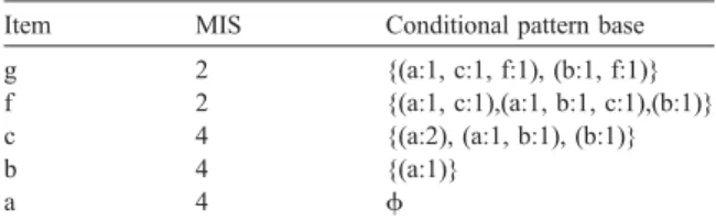
Fig. 6. g’s conditional MIS-tree. Table 3
Conditional pattern base
Item MIS Conditional pattern base g 2 {(a:1, c:1, f:1), (b:1, f:1)} f 2 {(a:1, c:1),(a:1, b:1, c:1),(b:1)} c 4 {(a:2), (a:1, b:1), (b:1)}
b 4 {(a:1)}
would be terminated. For cg and fg’s conditional pattern bases and conditional MIS-trees, we will find all the g’s conditional patterns (acg, afg, cfg, bfg) at level 3 and then try to construct their conditional pattern bases, respectively. The CFP-growth method for item g will not be terminated until all g’s conditional pattern bases contain no items. Repeatedly doing this for all items in the header table, we can get the whole conditional pattern base inTable 3and all conditional patterns inTable 4.
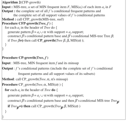
Fig. 7shows the detailed steps of the CFP-growth algorithm. In the following theorem, we show that the CFP-growth algorithm is both correct and complete. Here, bcorrectQ means every pattern output by the
algorithm is correct and bcompleteQmeans that every correct pattern will be output by the algorithm. However, to streamline the presentation we move the proof to Appendix A.
Theorem 1. The CFP-growth algorithm is correct
and complete.
Note that, when we have multiple MS, knowing the support of a frequent itemset does not imply that the supports of all its subsets are known. Thus, the MIS-tree differs from the FP-tree in that the FP-tree only contains frequent items in the tree while MIS-tree may contain infrequent items. If we only want to Table 4
All conditional patterns and conditional frequent patterns Item Conditional patterns Conditional
frequent patterns g ag, bg, cg, fg, acg, afg, cfg, bfg, acfg fg
f af, bf, cf, abf, acf, bcf, abcf af, bf, cf, abf, acf
c ac, bc, abc f
b ab f
Fig. 7. The CFP-growth algorithm. Table 5
The old and the new item order in the MIS-tree Item MIS value (old) MIS value (new) Old order New order Move-up item c Move-up item f a 4 5 1 2 c c b 4 3 2 4 a a c 4 6 3 1 b f f 2 4 4 3 f b g 2 2 5 5 g g
find all frequent patterns without considering the problem of rule generation, we can discard those infrequent items in the MIS-tree. However, in our CFP-growth method, we do the pattern growth for each item in the MIS-tree, so that not only frequent patterns but also the support values of all their subsets are found. Doing this enables us to obtain the support values of all conditional patterns.
5. Tuning MS
The primary challenge of devising an effective maintenance algorithm for association rules is how to reuse the original frequent itemsets and avoid the possibility of rescanning the original database DB[4]. In this study, we focus on the maintenance of the MIS-tree, so that every time after we tune the items’
supports, we can keep our MIS-tree in correct status without rescanning DB. The maintenance process can be stated as follows.
First, after the user tunes the items’ supports, we will get the new item order list in the MIS-tree. We need to determine which items should be moved up so that items in the MIS-tree can match the new item order. Notice that theMIN value is unchangeable during the support tuning process, and the MS of an item is not allowed to become either greater thanMINwhen it is smaller than MIN, or smaller than MIN when it is greater thanMIN. In other words, all the items in the MIS-tree must be kept the same after the tuning process.
We add this restriction for two reasons. First, with this restriction we do not need to access the database again when we change the minimum supports, because all the data needed to find frequent patterns are kept in the MIS-tree. This can greatly improve the performance of the support tuning mechanism. Sec-ond, this restriction does not present any real problem to the maintenance algorithm, because none of the
important patterns would be missing if we use a low
MIN value. (This restriction does not harm the applicability of the tuning algorithm, because by setting a low value of MIN the items’ supports can be tuned in a wide range).
InTable 5, we scan the items from the smallest old order to the largest one. If we find an item whose new order is smaller than its preceding items, then this item should be moved up. Continuously doing this, we can find all items that should be moved up. In Table 5, items c and f are two such items. As to item c, we see that the new order is 1. The items preceding c are items a and b, and their new orders
Table 6
Parameter settings for synthetic data generation |D| Number of transactions
|T| Average size of the transactions
|I| Average size of the maximal potentially frequent itemsets |L| Number of maximal potentially frequent itemsets N Number of items
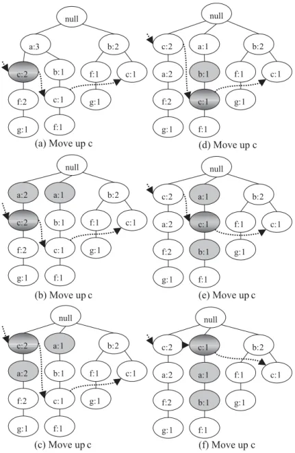
are 2 and 4. So we find that the new order of item c is smaller than that of item b and should be moved up. As to item f, we see that the new order of item f is 3. The items preceding f are items c, a and b, and their new orders are 1, 2 and 4. Since the new order of item f is smaller than item b, it should be moved up. After this scanning, we know we must do the move-up operation twice: firstly, to move-move-up item c, and, secondly, to move-up item f. After the first move-up operation, its order becomes the one shown in the first column of the right table inTable 5. Finally, the second move-up makes it become the one shown in the last column in Table 5.
Note that an item may occur several times in the MIS-tree, where all of them are linked together through its node-link. When we decide to move up an itemai, we first find the entry with item-name=aiin the MIN_frequent item header table and the head of its node-link. By traversing the node-link, we can visit all the nodes carrying the same item-name. In each visit, we move up the node of this item to the correct position. Let the node we are currently visiting be node
i, and let nodefbe the parent node of nodeiand node
gfthe grandparent of nodei. If the new order of nodef
is smaller than that of nodei, then the work is over. On the contrary, nodeishould be moved up above nodef. Here, if f.support=i.support, then we can directly swap these two nodes without any other modifications. However, iff.supportNi.support, then we split nodef into two nodes, nodef1and nodef2, wheref1.
suppor-t=i.support and f2.support=f.supporti.support. As for nodef1, we make nodeias its only child node, and then we swap node f1and nodei; as for nodef2, we make all child nodes of nodefexcept nodeias its child nodes; as for node gf, we make f1 and f2 as his children. This ascending process will be run repeatedly until the new order of the parent node is smaller than the currently visited node or until the parent node is the root. Fig. 8 shows how we finish the two move-up operations above.
After moving up these nodes, the nodes in MIS-tree may contain child nodes carrying the same item-name. For the sake of compactness, we use MIS_ merge method to merge those nodes. Following the Fig. 10. N1000-T10-I4-D0200K (MIN=0.01).
example in Fig. 8, the MIS_merge method can be illustrated inFig. 9.
6. Experimental evaluation
This section compares the performance of the MIS-tree algorithm and that of the MSapriori algorithm on both synthetic and real-life datasets. However, to understand more about the actual performance of these two algorithms we also include their counter-parts, i.e., the Apriori and the FP-growth algorithms, into our simulation. Since the last two algorithms are used for the single MS, we set all items’ supports as
MIN when executing them. In addition, we also investigated the performance of the maintenance algorithm for updating the MIS-tree when tuning MS. All experiments are performed on a Pentium 4 Celeron 1.8G PC with 768MB main memory, running on Microsoft Windows 2000 server. All the programs are written in Borland JBuilder7.
The synthetic data is generated by using the IBM data generator[1], which is widely used for evaluating
association rule mining algorithms. The parameters of the experiments are shown inTable 6. Besides, we use two datasets, BMS-POS and BMS-Webview-1, as our real-life dataset which was used in the KDD-Cup 2000 competition[15]. The BMS-POS dataset contains point-of-sale data from a large electronics retailer over seve-ral years. The transaction in this dataset is a customers’ purchase transaction, which consists of all the product categories purchased in a single round of shopping. The BMS-Webview-1 dataset contains several months of click stream data from an e-commerce website. Each transaction in this dataset is a web session consisting of all the product detail pages viewed in that session. That is, each product detail view is an item. We select these two datasets for comparison because they are repre-sentative of the typical data mining applications. So, they are suitable to measure the performance of the algorithm in a practical situation.
6.1. Experimental evaluation on four algorithms
In our experiments, we use the method proposed in Ref. [10]to assign MIS values to items. We use the
Fig. 13. N1000-T10-I4-D0400K (MIN=0.01). Fig. 12. N1000-T10-I4-D0200K (MIN=0.005).
actual frequencies of the items in theDBas the basis for MIS assignments. The formula can be stated as follows:
M(ai) is the actual frequency of item ai in the
DB. MIN denotes the smallest MIS value of all
items.r(0VrV1) is a parameter that controls how the MIS value for items should be related to their frequencies. If r=0, we have only one MS, MIN, which is the same as the traditional association rule mining.
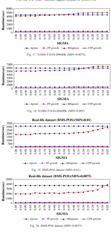
In the experiments, dataset N1000-T10-I4-D0200K is used in Figs. 10–12, N1000-T10-I4-D0400K used in Figs. 13–15, and N1000-T10-I4-D0600K used in
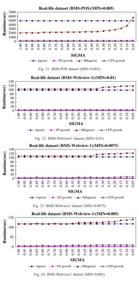
Figs. 16–18. These figures compare the run times of the four algorithms with respect tor. In addition, the two real datasets are compared inFigs. 19–24. From
Fig. 16. N1000-T10-I4-D0600K (MIN=0.01). Fig. 15. N1000-T10-I4-D0400K (MIN=0.005). Fig. 14. N1000-T10-I4-D0400K (MIN=0.0075).
MISð Þ ¼ai
Mð Þai Mð Þai NM I N
M I N otherwise Mð Þ ¼ai rfð Þai
Fig. 19. BMS-POS dataset (MIN=0.01). Fig. 18. N1000-T10-I4-D0600K (MIN=0.005). Fig. 17. N1000-T10-I4-D0600K (MIN=0.0075).
Fig. 22. BMS-Webview1 dataset (MIN=0.01).
Fig. 23. BMS-Webview1 dataset (MIN=0.0075).
Fig. 24. BMS-Webview1 dataset (MIN=0.005). Fig. 21. BMS-POS dataset (MIN=0.005).
all these figures, we see that our CFP-growth algorithm is about an order of magnitude faster than the MSapriori algorithm in all datasets.
To test the scalability with the number of trans-actions, we used the T10-I4-D0200K, N1000-T10-I4-D0400K and N1000-T10-I4-D0600K for our
experiments. TheMINvalue is set to 1% inFig. 25(a), 0.75% in Fig. 25(b) and 0.5% in Fig. 25(c). The reported run time is the average of the 20 tests forr from 0.05 to 1 (0.05, 0.1, 0.15,. . ., 0.95, 1). The experiments show that the run times of these four algorithms (Apriori, FP-tree, MSapriori, MIS-tree)
grow linearly when the number of transactions is increased form 200K to 600K. However, as the number of transactions is increased, the difference between (Apriori, MSapriori) and (FP-tree, MIS-tree) gets larger.
To test the scalability with MIN, we used the N1000-T10-I4-D0200K, N1000-T10-I4-D0400K and N1000-T10-I4-D0600K for our experiments. As in the preceding paragraph, the reported run time is the average value for 20 cases.Fig. 25(d–f) shows that the FP-growth and the CFP-growth algorithms have good scalability with respect to MIN. Besides, the FP-growth and CFP-FP-growth algorithms perform much better than the Apriori and MSapriori algorithm in scalability. This is because as we decrease the support threshold, the number of frequent itemsets increases dramatically; in turn, this makes the set of candidate itemsets used in the Apriori algorithm and the MSapriori algorithm become extremely large. So, the time increases rapidly as well.
All the experiments show that the CFP-growth algorithm is only a little slower than the FP-growth
method. This result is quite encouraging, for our algorithm does two more things than the FP-growth algorithm does—(1) we find frequent itemsets with multiple MS and (2) we find not only the supports of frequent itemsets but also the supports of all subsets of frequent itemsets.
6.2. Experiments for MS tuning
To test the performance of our tree maintenance algorithm when tuning MS, we compare it with the new construction of the MIS-tree. The reported run time is the average of the times spent in both synthetic and real-life datasets. TheMINvalue andrare set to 0.5% and 0.5, respectively. We randomly choose items in F with probability varied from 5% to 80%. The new MIS value of each chosen item will be set by randomly selecting a value from the range [old(10.05), old(1+0.05)], where old denotes the original MIS value. The results in Fig. 26 show that in average using our MIS-tree maintenance method is able to save more than 70% run time of
re-constructing the MIS-tree. Fig. 27 shows the scalability with MS tuning process. All experiments show that the saving is very significant in practice.
7. Conclusion
In this paper, we have developed an efficient algorithm for mining association rules with multiple MS and presented a maintenance mechanism for MS tuning without rescanning database. We have imple-mented the CFP-growth method and studied its performance in comparison with several frequent pattern mining algorithms. The results indicate that in all cases our algorithm is faster than the MSapriori algorithm. Besides, we also examined our mainte-nance algorithm for MS tuning. Experimental results show that our method is faster than the method of reconstructing the MIS-tree.
In short, the paper has three main results. First, we have developed an efficient algorithm for mining frequent patterns with multiple MS. Second, we solve the problem occurred in the MSapriori algorithm that it cannot generate association rules unless a post-processing phase is executed. Our method finds not only all frequent itemsets but also all subsets needed for generating association rules. Finally, we develop an efficient maintenance algo-rithm for updating the MIS-tree when the user tunes items’ MIS values.
The paper can be extended in several ways. First, we only consider the MIS-tree maintenance problem after the minimum supports are changed. Since the database is subject to update in practice, an interesting problem arising immediately is how to maintain the MIS-tree after the database is updated. In addition, we
may consider how to mine other kinds of knowledge under the constraint of multiple MS rather than setting a single MS threshold for all items. Because many kinds of knowledge that can be discovered from databases contain multiple items, all these types of knowledge can be extended naturally by setting different support thresholds for different items.
Acknowledgments
This research was supported in part by the Ministry of Education (MOE) Program for Promoting Aca-demic Excellence of Universities under Grant No. 91-H-FA07-1-4. We would like to thank anonymous referees for their helpful comments and suggestions.
Appendix A
Before giving the proof, we need to define the following terms.
Definition A.1. Let MIN denote the smallest MIS
value of all items. Then an item (itemset) is called MIN_frequent if its support is no less than MIN.
In addition, we briefly summarize the major steps of the CFP-growth algorithm as follows. This will enable us to ignore those details that are not related to the proof.
(1) LetTree denote the current MIS-tree,X denote the set of MIN_frequent patterns inTree and Y
denote the set of frequent patterns inTree. (2) Find all MIN_frequent items inTree. (3) For each MIN_frequent itemb inTree,
(3.1) Constructb’s conditional MIS-tree, denoted as
Treejb.
(3.2) Recursively find the set Xb of MIN_frequent itemsets inTreejb.
(3.3) ObtainXby appendingb after each pattern in
Xb.
(4) Put all those patternsxinXwhose supports are no less thanMIS(x) intoY.
(5) ReturnX.
First, the following theorem shows that the patterns found by the algorithm are correct, meaning that every Fig. 27. Scalability with MS tuning process.
pattern inXis MIN_frequent and every pattern inYis frequent.
Theorem A.1. The patterns obtained by the
CFP-growth algorithm are correct.
Proof. Because of the examination done in step 2,
every pattern in X must be MIN_frequent. Further, because of the examination done in step 4, every pattern inYmust be frequent. 5 Next, the following theorems show that the algorithm is complete, meaning that every MIN_fre-quent pattern and every freMIN_fre-quent pattern will be found by the algorithm.
Theorem A.2. The CFP-growth algorithm can find
every MIN_ frequent pattern.
Proof. Let (b1, b2,. . ., bk) denote the set of all
MIN_frequent items and they are arranged in non-increasing order according to their MIS values. Suppose X denote the set of MIN_frequent patterns in MIS-tree Tree. Then, we can partition X into k
subsets:
(1) the set of b1’s conditional MIN_frequent pat-terns; (includeb1only)
(2) the set of b2’s conditional MIN_frequent pat-terns; (must include b2; may include item bi, whereib2; but exclude all the others);
(3) the set of b3’s conditional MIN_frequent pat-terns; (must include b3; may include item bi, whereib3; but exclude all the others);. . . (k) the set of bk’s conditional MIN_frequent
patterns.
For each MIN_frequent item bi (ia[1. . .k]), we build bi’s conditional MIS-tree, denoted as Treejbi, fromTree.
We now prove this theorem by induction. Suppose we are given a MIN_frequent pattern denoted as
x=(bi1,bi2,. . .,bir), wherei1bi2b. . .bir. First, ifr=1, then there is only one single item inx. Since step 2 of the CFP-growth algorithm finds all MIN_frequent items, the algorithm will outputxas a MIN_frequent item.
Next, assume the algorithm can find all MIN_fre-quent patterns of no more than r1 items. And we now consider if the algorithm can find pattern x,
which hasritems. Sincexis a MIN_frequent pattern, the support of bir must be no less than MIN. This means step 3.1 of the algorithm will construct bir’s conditional MIS-treeTreejbir. In constructing the tree, by going through the bir’s node-link, all the trans-actions (built in the MIS-tree) related tobirwould be traversed. Hence, all the pattern information related to
bir will be kept in Treejbir. Further, by induction hypothesis, all the MIN_frequent patterns with no more than r1 items can be found from the tree. Thus, step 3.2 of the algorithm can find xV=(bi1,
bi2,. . .,bir1) fromTreejbir. Finally, step 3.3 will put these two parts, i.e., xVand bir, together; so, we can
find patternx. 5
Theorem A.2 shows that the algorithm can find all MIN_frequent itemsets. Since a frequent itemset must be a MIN_frequent itemset, we can find all frequent itemsets by checking if every MIN_frequent itemset satisfies the minimum item support constraint. Since we did so in step 4, the algorithm can find all frequent patterns. We list this result as the following theorem.
Theorem A.3. The CFP-growth algorithm can find
every frequent pattern.
Based on the three theorems above, we have the conclusion that the CFP-growth algorithm is correct and complete.
References
[1] R. Agrawal, R. Srikant, Fast algorithms for mining association rules, Proceedings of the 20th Very Large DataBases Conference (VLDB’94), Santiago de Chile, Chile, 1994, pp. 487 – 499.
[2] M.S. Chen, J. Han, P.S. Yu, Data mining: an overview from a database perspective, IEEE Transactions on Knowledge and Data Engineering 8 (1996) 866 – 883.
[3] W. Cheung, O.R. Zaiane, Incremental mining of frequent patterns without candidate generation or support constraint, Proceedings of the 7th International Database Engineering and Applications Symposium (IDEAS’03), Hong Kong, 2003, pp. 111 – 116.
[4] D. Cheung, J. Han, V. Ng, C.Y. Wong, Maintenance of discovered association rules in large databases: an incremental updating technique, Proceedings of International Conference on Data Engineering (ICDE’96), New Orleans, LA, USA, 1996, pp. 106 – 114.
[5] R. Feldman, Y. Aumann, A. Amir, H. Mannila, Efficient algorithm for discovering frequent sets in incremental data-bases, Proceedings of SIGMOD Workshop on Research Issues
in Data Mining and Knowledge Discovery (DMKD’97), Tucson, AZ, USA, 1997, pp. 59 – 66.
[6] J. Han, Y. Fu, Discovery of multiple-level association rules from large databases, Proceedings of the 21th Very Large DataBases Conference (VLDB’95), Zurich, Switzerland, 1995, pp. 420 – 431.
[7] J. Han, M. Kamber, Data Mining: Concepts and Techniques, Morgan Kaufmann Publisher, San Francisco, CA, USA, 2001. [8] J. Han, J. Pei, Y. Yin, Mining frequent patterns without candidate generation, Proceedings 2000 ACM-SIGMOD International Conference on Management of Data (SIG-MOD’00), Dallas, TX, USA, 2000.
[9] W. Lee, S.J. Stolfo, K.W. Mok, Mining audit data to build intrusion detection models, Proceedings of the 4th Interna-tional Conference on Knowledge Discovery and Data Mining (KDD ’98), New York, NY, USA, 1998.
[10] B. Liu, W. Hsu, Y. Ma, Mining association rules with multiple minimum supports, Proceedings of the ACM SIGKDD International Conference on Knowledge Discovery and Data Mining (KDD-99), San Diego, CA, USA, 1999.
[11] H. Mannila, Database methods for data mining, Proceedings of the 4th International Conference on Knowledge Discovery and Data Mining (KDD ’98) tutorial, New York, NY, USA, 1998. [12] V. Pudi, J.R. Haritsa, Quantifying the utility of the past in mining large databases, Information Systems 25 (5) (2000) 323 – 343.
[13] S. Thomas, S. Bodagala, K. Alsabti, S. Ranka, An efficient algorithm for the incremental update of association rules in large database, International Conference on Knowledge Dis-covery and Data Mining (KDD’97), Newport, CA, USA, 1997.
[14] M.C. Tseng, W.Y. Lin, Mining generalized association rules with multiple minimum supports, International Conference on Data Warehousing and Knowledge Discovery (DaWaK’01), Munich, Germany, 2001, pp. 11 – 20.
[15] Z. Zheng, R. Kohavi, L. Mason, Real world performance of association rule algorithms, Proceedings of the 7th ACM-SIGKDD International Conference on Knowledge Discovery and Data Mining, San Francisco, CA, USA2001, pp. 401 – 406.
Ya-Han Huis currently a PhD student in the Department of Information Manage-ment, National Central University, Taiwan. He received the MS degree in Information Management from National Central Uni-versity of Taiwan. His research interests include data mining, information systems and EC technologies.
Yen-Liang Chenis Professor of Informa-tion Management at NaInforma-tional Central Uni-versity of Taiwan. He received his PhD degree in computer science from National Tsing Hua University, Hsinchu, Taiwan. His current research interests include data modeling, data mining, data warehousing and operations research. He has published papers in Decision Support Systems, Oper-ations Research, IEEE Transaction on Software Engineering, IEEE Transaction on Knowledge and Data Engineering, Computers and OR, Euro-pean Journal of Operational Research, Expert Systems with Applications, Information and Management, Information Processing Letters, Information Systems, Journal of Operational Research Society, and Transportation Research.