Scalable posterior approximations for large-scale Bayesian inverse problems
via likelihood-informed parameter and state reduction
Tiangang Cuia, Youssef Marzouka,∗, Karen Willcoxa aMassachusetts Institute of Technology, Cambridge, MA 02139, USA
Abstract
Two major bottlenecks to the solution of large-scale Bayesian inverse problems are the scaling of posterior sampling algorithms to high-dimensional parameter spaces and the computational cost of forward model evaluations. Yet incomplete or noisy data, the state variation and parameter dependence of the forward model, and correlations in the prior collectively provide useful structure that can be exploited for dimension reduction in this setting—both in the parameter space of the inverse problem and in the state space of the forward model. To this end, we show how to jointly construct low-dimensional subspaces of the parameter space and the state space in order to accelerate the Bayesian solution of the inverse problem. As a byproduct of state dimension reduction, we also show how to identify low-dimensional subspaces of the data in problems with high-dimensional observations. These subspaces enable approximation of the posterior as a product of two factors: (i) a projection of the posterior onto a low-dimensional parameter subspace, wherein the original likelihood is replaced by an approximation involving a reduced model; and (ii) the marginal prior distribution on the high-dimensional complement of the parameter subspace. We present and compare several strategies for constructing these subspaces using only a limited number of forward and adjoint model simulations. The resulting posterior approximations can rapidly be characterized using standard sampling techniques, e.g., Markov chain Monte Carlo. Two numerical examples demonstrate the accuracy and efficiency of our approach: inversion of an integral equation in atmospheric remote sensing, where the data dimension is very high; and the inference of a heterogeneous transmissivity field in a groundwater system, which involves a partial differential equation forward model with high dimensional state and parameters.
Keywords: Inverse problems, Bayesian inference, dimension reduction, model reduction, low-rank approximation, Markov chain Monte Carlo
1. Introduction
Inverse problems convert indirect observations into useful characterizations of the parameters of a physical system. These parameters are related to the observations by a forward model, which often is expressed as a system of ordinary or partial differential equations (PDEs) or as an integral equation. Observations are inevitably corrupted by noise, and the unknown model parameters
∗
Corresponding author
Email addresses: [email protected](Tiangang Cui),[email protected](Youssef Marzouk),[email protected]
(Karen Willcox)
may be high-dimensional or infinite-dimensional in principle. Solution of the inverse problem is thus classically ill-posed: many feasible realizations of the parameters may be consistent with the data, and small perturbations in the data may lead to large perturbations in unregularized parameter estimates. Rather than seeking regularized point estimates, the Bayesian approach [1,2,3] casts the inverse solution as theposterior probability distribution of the model parameters conditioned on data, and introduces regularization in the form of prior information. It thus provides a means of combining prior knowledge, the data and forward model, and a stochastic description of measurement and/or model errors; the result is a principled quantification of uncertainty in parameters and in parameter-dependent predictions. Characterizing the posterior, however, is in general a computationally challenging task. The workhorses of Bayesian computation in this context are Markov chain Monte Carlo (MCMC) methods [4,5,6], originating with the Metropolis-Hastings algorithm [7,8].
A central challenge in the application of MCMC methods to inverse problems is poor scal-ing of computational effort with parameter dimension and with the size of the forward model. High-dimensional parameters frequently represent the discretization of a spatial field (e.g., the permeability field of a porous medium) that is the target of inference. Yet the efficiency of many standard MCMC methods degrades with parameter dimension [9, 10, 11, 12, 13]; longer mixing times for MCMC chains then demand more posterior evaluations to estimate posterior expecta-tions with any given accuracy. Similarly, many forward models of interest have high-dimensional states—resulting, for instance, from finite-element discretizations of PDEs, where many degrees of freedom are needed to resolve the relevant physics accurately. The computational expense of each forward model evaluation scales at least linearly with the dimension of model state (e.g., when the solution of a linear system is required). Another important but often-neglected computational expense in MCMC methods is the proposal process: the cost of generating random variables and calculating the candidate step often scales at least linearly with the parameter dimension.
To overcome these twin challenges—parameter dimension and forward model cost—this paper proposes a likelihood-informed approach for identifying and exploiting low-dimensional structure in both the parameter space and the model state space of inverse problems. Our approach inte-grates and extends two lines of research: the likelihood-informed parameter dimension reduction of [14,15] and the data-drivenmodel reduction of [16]. By simultaneously considering the limited accuracy or influence of the observations, the smoothing properties of the forward model, and the covariance structure of the prior, the former identifies a low-dimensional likelihood-informed parameter subspace(LIPS)1 where the influence of the likelihood on the posterior dominates that of the prior. Given this subspace, one can approximate the full posterior2 as the product of a low-dimensional posterior on the LIPS and the marginalization of the prior onto the complement of the LIPS. The latter term can be characterized analytically or with perfectly independent sam-ples. Evaluation of the posterior density restricted to the LIPS is still computationally expensive, however, as it involves the full forward model. Our second step accelerates these evaluations by projecting [18,19,20,21] the forward model—with input parameters restricted to the LIPS—onto a low-dimensional state subspace. This subspace is called the likelihood-informed state subspace
1
[15] and [17] refer to this reduced parameter subspace as the “likelihood-informed subspace” or LIS. Since the present work introduces low-dimensional subspaces of both the parameter space and state space, we replace ‘LIS’ with the more specific ‘LIPS’ in order to avoid confusion.
2The term “full posterior” refers to the posterior distribution induced by the full forward model defined on the
(LISS), as it captures variations in the model state associated with the LIPS-projected posterior. This model reduction approach extends the data-driven model reduction ideas of [16] by not only exploiting posterior concentration, but also avoiding consideration of input parameter directions that ultimately will not be data-informed. Finally, we combine these approximations together: the reduced-order model resulting from projection onto the LISS is substituted into the product-form approximation of the posterior described above. The resulting jointly-approximated posterior is inexpensive to evaluate and to sample, with a computational cost that is independent of the di-mension of the full model state or the parameters. Indeed, this cost scales only with the didi-mensions of the LIPS and the LISS, which are in a sense theintrinsic dimensions of the problem.
As a byproduct of state reduction, we describe new approaches for efficiently handling and reducinghigh-dimensional data sets in inverse problems; these approaches are potentially useful in “big data” settings. While the jointly-approximated posterior achieves excellent accuracy in our numerical examples, we also discuss how to use it as a proposal distribution in importance sampling or delayed-acceptance MCMC [22,23] for the purpose of “exact” sampling—i.e., the computation of expectations with respect to the full posterior—if desired. To ensure convergence in this setting, we introduce a special treatment of the tails of the jointly-approximated posterior.
Previous work has also investigated the idea of combining parameter reduction with model re-duction or other forms of surrogate modeling in order to approximate posterior distributions. One early effort is [24], which constructs a reduced parameter basis using the truncated Karhunen-Lòeve (KL) expansion [25,26] of the prior covariance, and then uses generalized polynomial chaos expan-sions [27,28,29] to build a surrogate of the full model. The same KL-based parameter reduction technique has also been combined with projection-based model reduction to accelerate posterior evaluations; examples include [30] and [16]. Similarly, [31] combines a process convolution model [32] of the parameters with a sparse grid approximation of the forward model. A different approach in [33] simultaneously identifies reduced subspaces for both the parameters and the state, by solv-ing a sequence of model-constrained optimization problems penalized by the prior. In general, all these earlier approaches seek a truncation of the parameter dimension and then accelerate forward model evaluations over the reduced parameter subspace using surrogates. The smoothness of the prior plays a crucial role in these approaches, either for avoiding large KL truncation errors or for promoting convergence of the model-constrained optimization. In practice, this requirement can impose significant restrictions on the choice of priors. Our approach is fundamentally different in several respects. First, our posterior approximation is based on capturing the change from the prior to the posterior within the LIPS, rather than directly truncating the parameter dimension of the problem. Second, model reduction using the LISS only captures the state variations that are relevant to the change from prior to posterior; this “localization” strategy is key to the successful construction of reduced-order models for high-dimensional parameterized systems. Furthermore, our jointly-approximated posterior is not singular with respect to the full posterior, and can thus be used to drive exact sampling schemes (e.g., importance sampling as mentioned above).
The rest of this paper is organized as follows. In Section2, we review the Bayesian formulation of inverse problems. In Section3, we introduce the concept of joint posterior approximation using reduced parameter and state subspaces, then detail various strategies and practical algorithms for constructing this approximation and for exploring the full posterior. In Section4, we demonstrate various aspects of our proposed approach using an atmospheric remote sensing problem, comparing different strategies for subspace identification and for the reduction of high-dimensional data. In Section5, we apply our joint posterior approximation approach to the inference of the transmissivity
field of a groundwater aquifer. Section6offers concluding remarks.
2. Bayesian formulation for inverse problems
We begin by constructing the forward model. Consider a numerical discretization of the system of interest, described by a nonlinear equation
A(u, x) = 0, (1)
whereu∈U⊆Rm andx∈
X⊆Rn are them-dimensional state vector and then-dimensional pa-rameter vector, respectively. The goal of an inverse problem is to infer the unobservable papa-rameters
x from noisy partial observations of the statesu, given by
yobs=C(u, x) +e . (2)
Here C is a discretized observation operator mapping from the states and parameters to the ob-servables, and e is a random variable representing noise and/or model error, which appear addi-tively. The system model A(u, x) = 0 and observation model C(u, x) together define a forward model y = F(x) that maps the unknown parameter to the observable model outputs. We note that although the forward model defined by (1) and (2) is induced by a stationary problem, the methodology presented in this paper is also applicable to time-dependent systems.
To formulate the inverse problem in a Bayesian setting, we model the parameterxas a random variable, endow it with a prior distribution, and then characterize its posterior distribution given a realization of the data,yobs ∈Y⊆Rd:
π(x|yobs)∝ L(yobs|x)π0(x). (3)
Here, we assume that all distributions have densities with respect to Lebesgue measure. The poste-rior density above is the product of two terms: the pposte-rior densityπ0(x), which models knowledge of
the parameters before the data are observed, and the likelihood functionL(yobs|x), which describes
the probability distribution ofyobs for a given x.
We develop our formulation in the setting of a multivariate Gaussian prior N(µpr,Γpr), where
the covariance matrix Γpr might also be specified by its inverse Γ−1pr, commonly referred to as the
precision matrix. The additive observational noise is taken to be a zero mean Gaussian distribution, i.e., e∼ N(0,Γobs). Given the weighted inner product hy1, y2iΓobs =hy1,Γ
−1
obsy2i and the induced
norm kykΓobs =qhy, yiΓobs, we can define a data-misfit function
η(x) = 1
2kF(x)−yobsk
2
Γobs. (4)
The likelihood function is thus proportional to exp (−η(x)). The Gaussian settings used here can be generalized to non-Gaussian priors, e.g., log-normal distributions, with an appropriate transformation or change of variables to a Gaussian. Additive but non-Gaussian noise can be handled similarly. These transformations may introduce additional nonlinearity in the forward model.
Note that the unknown parameters and the model states are in principle functions of space and/or time, and that the finite-dimensional representations above are the result of numerical discretization. If one considers progressively refining the parameter discretization, however, the
posterior distribution does not have a density with respect to Lebesgue measure at the infinite-dimensional limit. However, for inverse problems with properly chosen Gaussian priors—e.g., a covariance operator that is self-adjoint, positive definite, and trace-class—and a forward model satisfying certain regularity conditions—e.g., appropriately bounded [3] and locally Lipschitz—the posterior has a density with respect to the prior and yields a full measure at the infinite-dimensional limit. In this case, Bayes’ rule in (3) is expressed as the Radon-Nikodym derivative of the posterior with respect to the prior. We refer the readers to [3] and references therein for more details. Since we aim to approximate the posterior distribution defined by given discretizations of the parame-ters, a finite-dimensional forward model, and the associated prior, we adopt the finite-dimensional representation of the posterior as our starting point in this paper. This finite-dimensional posterior can be derived either from a consistent discretization of an infinite-dimensional inverse problem or from some other existing numerical models that are not necessarily well-defined in the infinite-dimensional limit.
3. Posterior approximation via dimension reduction
In this section, our first objective is to reduce the algorithmic complexity of posterior sampling by identifying a likelihood-informed parameter subspace (LIPS) that captures parameter directions where the change from prior to posterior is most significant. We will then decompose the posterior into the product of (i) a low-dimensional distribution, defined on the LIPS, that is analytically intractable and therefore must be sampled; and (ii) a higher-dimensional but analytically tractable marginal of the prior distribution on the complement of the LIPS. To accelerate the forward model evaluations required when sampling the first term of this product decomposition, we will identify a low-dimensional subspace of the forward model state—the likelihood-informed state subspace (LISS)—and construct a reduced version of the forward model accordingly. Introducing this re-duced model into the product decomposition yields the jointly-approximated posterior distribution described in the introduction. At the end of this section, we will describe and compare various sampling strategies for constructing the LISS and LIPS, and hence the jointly-approximated poste-rior. We will also discuss methods for exploring the full posterior distribution, given the preceding approximations.
3.1. Data-informed parameter reduction
Inverse problems very often involve some combination of a smoothing forward model, limited or noisy observations, and correlations in the prior. When any of these factors is present, the data will not equally inform all directions in the parameter space. We may be able to explicitly project the argument of the likelihood function onto a lower-dimensional subspace of the parameter space without losing much information. Our objective here is to find anr-dimensional LIPS, denoted by Xr, to capture the parameter directions where the likelihood is “most informative” relative to the
prior. This notion will be defined more precisely below.
3.1.1. Parameter-reduced posterior
Consider a rank-r projector Πrwhose range is the LIPS, i.e.,Xr = range(Πr). We approximate
the posterior density (3) as: ˆ
π(x|yobs)∝ L(yobs|Πrx)π0(x), (5)
where L(yobs|Πrx) is an approximation to the original likelihood function L(yobs|x). We require
hx1, x2iΓpr = hx1,Γ
−1
prx2i. This requirement is essential to constructing a tractable product-form
approximation of the posterior.
Definition 3.1 (Parameter space projectors). Suppose the subspace Xr is spanned by a basis
Φr∈Rn×r that is orthogonal with respect to the inner producth·,·i
Γpr, i.e.,hΦr,ΦriΓpr =Ir, where
Ir is the r-by-r identity matrix. Define the matrix Ξr ∈ Rn×r such that Ξ>rΦr = Ir. Then the
projectors
Πr= ΦrΞ>r and Π⊥=I−Πr,
are orthogonal with respect toh·,·iΓpr. Moreover, the(n−r)-dimensional subspaceX⊥= range(Π⊥) is the orthogonal complement of Xr with respect to h·,·iΓpr. We can choose a basis Φ⊥∈Rn×(n−r)
such that [Φr,Φ⊥] forms a complete orthogonal system in Rn with respect to h·,·iΓpr, and thus
the projector Π⊥ can be written as Π⊥ = Φ⊥Ξ>⊥, where Ξ⊥ ∈ Rn×(n−r) is the matrix such that Ξ>⊥Φ⊥=I⊥.
Using the projectors defined above, the parameter x can be decomposed as x = Πrx+ Π⊥x,
where each projection can be represented as the linear combination of the corresponding basis vectors. Consider parameters xr and x⊥ that are the weights associated with the bases Φr and
Φ⊥, respectively. Then we can define the following pair of linear transformations between x and
(xr, x⊥): x= [ΦrΦ⊥] " xr x⊥ # and " xr x⊥ # = [ΞrΞ⊥]>x. (6)
Lemma 3.2. Given the decomposition x = Φrxr+ Φ⊥x⊥ defined in (6), the prior distribution can be decomposed into the product form π0(x)∝π0(xr)π0(x⊥), where π0(xr) =N(Ξ>rµpr, Ir) and
π0(x⊥) =N(Ξ>⊥µpr, I⊥).
Applying the linear transformation (6) and Lemma3.2, the parameter-approximated posterior (5) can be written as
ˆ
π(x|yobs)∝πˆ(xr, x⊥|yobs) =π(xr|yobs)π0(x⊥), (7)
which is the product of theparameter-reducedposterior
π(xr|yobs)∝ L(yobs|Φrxr)π0(xr), (8)
and the complement prior π0(x⊥). In this product-form approximation, the prior-to-posterior
update is captured entirely by the parameter-reduced posterior. Approximations of this form nat-urally yield a scalable posterior exploration scheme: the high-dimensional complement priorπ0(x⊥)
is analytically tractable, and the remaining challenge is to explore the analytically intractable but low-dimensional parameter-reduced posterior (8). Of course, this construction rests on identifying the LIPS basis Φr. In the rest of this subsection, we will discuss several ways to construct the LIPS by balancing the influence of the prior and the likelihood.
Remark 3.3. It is usually not feasible to compute and store the high-dimensional basis Φ⊥ ∈
Rn×(n−r). In fact, the construction of the parameter-approximated posterior (7) only requires the
low-dimensional LIPS basis Φr in order to construct the parameter-reduced posterior. Operations involving the complement subspaceX⊥ are performed using the projectorΠ⊥=I−Πr rather than
3.1.2. Likelihood-informed parameter subspace
In previous work [14,34,35,36,37], the Hessian of the data-misfit function (4) (in particular, the Gauss-Newton approximationH(x) of the Hessian) is used to quantify the local impact of the likelihood, relative to the prior, along a parameter direction ϕ. This notion of relative impact is captured via the local Rayleigh ratio
R(ϕ;x) = hϕ, H(x)ϕi hϕ,Γ−1prϕi
, (9)
which is maximized (over successively smaller subspaces span⊥(ϕj)j<i) by generalized eigenvectors
of the matrix pencil (H(x),Γ−1pr)
H(x)ϕi =γiΓ−1prϕi. (10) The largest eigenvalues of (10) correspond to parameter directions along which the local curva-ture of the log-posterior density is more constrained by the log-likelihood than by the log-prior. Conversely, eigendirections associated with the smallest eigenvalues correspond to directions along which the likelihood is essentially flat, and hence where the posterior is (locally) determined by the prior.
Given the local Gauss-Newton approximation of the Hessian,H(x), we can define a local Gaus-sian approximation of the posterior with covariance Γpos(x) := (H(x) + Γ−1pr)−1. This covariance can be written as a low-rank update of the prior covariance:
Γpos(x)≈Γ(posl) = Γpr− l X i=1 γi γi+ 1ϕiϕ > i , (11)
which is in general approximate for l < n. Here ϕi and γi are eigenvectors and eigenvalues from
(10), which depend on the parameterx. In this approximation, the basis{ϕ1, . . . , ϕl}characterizes
the prior-to-posterior update at a givenx.
This low-rank update was first used in [34] for computing and factorizing the posterior co-variance in large-scale linear inverse problems. Spantini et al. [14] proved the optimality of this approximation at any givenl, for linear inverse problems, in the sense of minimizing the Förstner-Moonen [38] distance from the exact posterior covariance matrix over the class of positive definite matrices that are rank-lnegative semidefinite updates of the prior covariance. For nonlinear inverse problems, given the posterior mode (i.e., the maximum a posteriori (MAP) estimator)
xMAP= arg max
x
π(x|yobs),
the local Gaussian approximation (11) centered at xMAP yields a Laplace approximation of the
posterior:3 π(x|yobs)≈πL(x) =N xMAP,Γpr− l X I=1 γi γi+ 1ϕiϕ > i ! . (12)
For unimodal and nearly Gaussian posteriors, the Laplace approximation might be used directly as a surrogate for the posterior, as in [36]; alternatively, it can be used as a fixed preconditioner
3More precisely, this is a Laplace approximation with an additional approximation of the covariance as a low-rank
for MCMC sampling, as in the stochastic Newton method of [37]. We will use the Laplace ap-proximation as a component of certain subspace construction strategies, described in the next subsection.
We wish to construct the parameter-approximated posterior (7) for nonlinear inverse problems, and thus must extend beyond Gaussian approximations. Since the Hessian varies over the parame-ter space for nonlinear forward models, the likelihood-informed directions also vary withxand are embedded in some nonlinear manifold. To build a global linear subspace—the LIPS—that captures the majority of this nonlinear manifold, Cui et al. [15] extends the pointwise criterion (9) into the expected value of the Rayleigh quotient over the posterior
Eπ(x|yobs)[R(φ;x)] =
hφ, Spostφi
hφ,Γ−1prφi
, (13)
whereSpostis the posterior expectation of the Gauss-Newton approximation of the Hessian (GNH):
Spost=
Z
X
H(x)π(dx|yobs). (14)
This way, the LIPS can be obtained through the eigendecomposition of the matrix pencilSpost,Γ−1pr
,
Spostφi =λiΓ
−1
prφi. (15)
The eigenvectors{φ1, . . . , φr}correspond to ther leading eigenvalues of (15), such thatλ1 ≥λ2≥
. . . ≥ λr ≥ τg > 0, span the LIPS. Here the truncation threshold τg is usually set to a value
less than one, e.g., τg = 10−1, thus only removing parameter directions where the impact of the
likelihood is significantly smaller than that of the prior.
The evaluation of the expected GNH (14) should be carried out adaptively during posterior exploration. In particular, we consider approximating Spost using Monte Carlo integration,
b Spost= 1 N N X k=1 H(x(k)), where x(k) ∼ π(x|y
obs), k = 1. . . N, are posterior samples adaptively selected during posterior
exploration. Section 3.3 will describe how we fit this task into an adaptive sampling framework where posterior exploration and posterior approximation are carried out simultaneously.
Lemma 3.4. The eigenvectors {φ1, . . . , φr} are linearly independent and form a LIPS basis Φr=
[φ1, . . . , φr] that is orthogonal with respect to the inner producth·,·iΓpr.
Proof. The result directly follows from the fact that the estimated expected GNHSbpostis symmetric positive semidefinite and the prior covariance Γpris symmetric positive definite. See Theorem 15.3.3
of [39] for details.
As a consequence of Lemma 3.4, we can construct the matrix Ξr = Φr(Φ>r Φr)−1, such that Ξ>rΦr = Ir, and the projector Πr = ΦrΞ>r as in Definition 3.1. This way, the
3.1.3. Parameter subspace identification: choice of reference distribution
The LIPS basis discussed above results from balancing the influence of the prior and the likeli-hood over the support of the posterior. It is also possible to quantify this relative influence using expectations of the local Rayleigh quotient over other reference distributions. Depending on the choice of reference distribution, the local likelihood-informed directions—summarized by the local Rayleigh quotient—are weighed differently in the resulting LIPS. Furthermore, the involvement of the observed data set in the reference distribution affects how computational resources might be allocated to LIPS construction. If the observed data are not involved in the reference distribution, the evaluation of the expectation can be performed once for a particular combination of forward model and prior, and reused for different data sets.4 This way, LIPS construction is decoupled from any particular data set, and we consider it to be anofflineprocedure. In contrast, if the ref-erence distribution involves the observation—e.g., if it is the posterior—the resulting expectation evaluation is an online procedure, as the LIPS basis must be recomputed for each new data set.
One obvious candidate for the reference distribution is the prior, which leads to a LIPS basis that is constructed from the eigendecomposition of the matrix pencilSpr,Γ−1pr
, where Spr = Z X H(x)π0(dx),
is the expected GNH over the prior. As discussed above, using the prior as a reference distribution leads to an offline procedure for parameter dimension reduction.
Alternatively, we can set the reference distribution to be the Laplace approximation (12), which is an inexpensive and easy-to-sample surrogate for the posterior. This way, the LIPS can be obtained from the eigendecomposition of the pencil SL,Γ−1pr
, where SL= Z X H(x)πL(dx).
Although samples can be directly drawn from the Laplace approximation, this choice of reference constitutes an online approach, since the Laplace approximation is data-dependent.
All of the LIPS bases discussed above are orthogonal with respect to the inner producth·,·iΓpr, since they result from generalized eigenproblems involving Γ−1pr. We note that other choices of reduced parameter basis can also lead to the product-form approximated posterior (7), provided that the basis is orthogonal with respect toh·,·iΓpr. For instance, the basis defined by the truncated Karhunen-Loève expansion of the prior covariance [24] also satisfies this property.
All of the parameter subspace identification techniques presented here can be interpreted as the result of an eigendecomposition. For each technique, Table 1 summarizes the specific form of eigendecomposition, whether reduction is offline/online, and whether adaptive sampling is re-quired. We compute the expected Hessians required for both Prior-LIPS and Laplace-LIPS using Monte Carlo integration, where samples can be directly generated from the prior and the Laplace approximation. These Hessian evaluations are therefore embarrassingly parallel. Posterior-LIPS, on the other hand, requires posterior sampling; we defer a discussion of the associated adaptive framework to Section3.3. We also note that Prior-KL is less computationally demanding than the other methods discussed here, as it only involves an eigendecomposition of the prior covariance.
Table 1: Summary of parameter dimension reduction methods discussed in Section3.1.3: the associated eigende-composition, whether the process is offline/online, and whether adaptive sampling is required.
Method Eigendecomposition Online/offline Adaptive sampling?
Posterior-LIPS Spost,Γ−1pr
Spost=RXH(x)π(dx|yobs) online yes
Laplace-LIPS SL,Γ−1pr SL=RXH(x)πL(dx) online no Prior-LIPS Spr,Γ−1pr Spr =RXH(x)π0(dx) offline no Prior-KL Γpr – offline no 5 x1 0 (a):y=F(x) -5 -5 0 x2 10 5 0 5 (b): π 1 x|y(1)o 2 x1 -4 -3 -2 -1 0 1 x2 -4 -3 -2 -1 0 1 (c): π 1 x|yo(2) 2 x1 0 1 2 3 4 5 x2 0 1 2 3 4 5
Figure 1: Illustration of Example3.5. (a) Forward model, with two different observations yobs(1) and y(2)obs marked by the triangle and the circle, respectively. (b) Contours of the posterior densityπ(x|yobs(1)). (c) Contours of the posterior densityπ(x|yobs(2)). On (b) and (c), the parameter bases computed using posterior-LIPS, Laplace-LIPS, and prior-LIPS are depicted by the solid, dashed, and dotted lines, respectively.
Example 3.5 (Parameter reduction with different reference distributions). To demonstrate the properties of different parameter reduction approaches, we consider a two-dimensional inverse prob-lem with the following scalar-valued forward model:
F(x) := 1
2[(erf (x1+ 1) + 1) (x1+ 1) + (erf (x2+ 1) + 1) (x2+ 1) + (1−erf (x1+ 1)) cos(x2)].
We define a Gaussian observational error e ∼ N(0, σ−2I1) with σ = 0.25, and a prior π0(x) =
N(0, I2). Figure 1(a) shows the response of the forward model over a range of input parameter values (x1, x2). Different observations will yield posterior distributions with dramatically different shapes and orientations, due to the nonlinearity of the forward model. We consider two different observation values y(1)obs and yobs(2), generated by setting the underlying true parameter to (−1,−2)
and (3,3), respectively. These observations are illustrated by the triangle and the circle in Figure
1(a).
As shown in Figure 1(b), the posterior distribution π(x|y(1)obs) has strongly non-Gaussian struc-ture in both parameter dimensions, as the observationyobs(1) falls in a regime where the forward model exhibits nonlinear behavior. In contrast, the observation yobs(2) corresponds to a parameter regime
where the forward model is rather linear, and thus the posterior distribution π(x|yobs(2)), shown in Figure1(c), has nearly Gaussian structure.
In this example, the Prior-KL basis simply corresponds to the canonical basis of the posterior, as the prior is an independent standard Gaussian. The Prior-LIPS basis is illustrated with dotted lines and remains unchanged for both data sets, while the Posterior-LIPS basis is illustrated with solid lines and depends on the data set. The vectors corresponding to the Prior-LIPS basis and the Posterior-LIPS basis in the figure are scaled by their associated generalized eigenvalues. For the data setyobs(2), the likelihood function only informs one dimension in the parameter space, since the forward model is nearly linear in the support of the posterior. Posterior-LIPS captures this likelihood-informed subspace accurately, but Prior-LIPS does not; it suggests that two parameter directions are of comparable importance. Laplace-LIPS produces results similar to Posterior-LIPS for the data set y(2)obs, but the bases generated by Laplace-LIPS and Posterior-LIPS are rather dif-ferent for the data set yobs(1). This is expected, because the posterior π(x|yobs(2)) is nearly Gaussian and well described by its Laplace approximation, whereas the posterior π(x|y(1)obs) is strongly non-Gaussian.
As shown by the above example, all three strategies for computing the LIPS can reveal the impact of the likelihood on different parameter directions, relative to the prior. The Prior-LIPS does not depend on the data set, and hence can be constructed offline for all possible observations. Its potential drawback is that the resulting low-dimensional parameter subspace may contain directions unimportant to the posterior at hand; alternatively, some important posterior structure may be missed, due to the averaging of different Hessians over a much less concentrated parameter measure. In comparison, the online Posterior-LIPS can accurately capture likelihood-informed directions for a specific posterior distribution of interest. Depending on the shape of the posterior, Laplace-LIPS can be used either as a replacement for Posterior-LIPS when the posterior is nearly Gaussian, or as an initial guess for Posterior-LIPS that is adaptively refined (see Section3.3).
3.2. Likelihood-informed state reduction
Although the parameter-approximated posterior ˆπ(x|yobs) ∝ π(xr|yobs)π0(x⊥) enables
signifi-cant reductions in the algorithmic complexity of posterior exploration, by confining sampling to a lower dimensional space, a remaining computational bottleneck is the exploration of the parameter-reduced posteriorπ(xr|yobs). The cost of this exploration is dominated by forward model
evalua-tions, and thus we turn to model reduction approaches.
3.2.1. Model reduction
In the parameter-reduced posterior, by projecting the argument of the likelihood function onto the subspace spanned by the reduced parameter basis Φr, the forward model defined by (1) and (2) can be rewritten as
A(u,Φrxr) = 0, and y=C(u,Φrxr). (16)
To reduce the computational cost, we wish to solve a projection of the parameter-reduced forward model (16) onto a reduced dimensional state subspace. Without loss of generality, we consider the system modelA(u, x) = 0 to consist of a linear operatorL and a nonlinear functionf, which take the form
Suppose that variation of them-dimensional state lies within an s-dimensional subspace spanned by a basisVs ∈Rm×s. Then the stateucan be approximated by a linear combination of the reduced basis vectors, i.e., u ≈Vsus. This way, the parameter-reduced system model A(u,Φrxr) = 0 can
be approximated by the following Galerkin projection:
Vs>L(Φrxr)Vs
| {z }
Ls(xr)
us+Vs>f(Vsus,Φrxr) = 0. (18)
Ifsm, the dimension of the unknown state in (18) is greatly reduced compared to that of the original system (17). However, (18) cannot necessarily be solved quickly, because the reduced-order model still requires evaluating the full-scale system matrices or residual and then projecting those matrices or the residual onto the reduced state subspace. Many elements of these computations depend on the state and parameter dimension of the original system, and hence this process is typically computationally expensive (unless there is special structure to be exploited, such as affine parametric dependence). In this situation, methods such as missing point estimation [40], empirical interpolation [41], or its discrete variant [42], can be used to approximate the nonlinear term in the reduced-order model by selective spatial sampling.
We employ the discrete empirical interpolation method (DEIM) [42] to approximate the non-linear terms of (18). Suppose that the outputs of a nonlinear function f(Vsus,Φrxr) in (18) can
be captured by a linear subspace spanned by the basis Θt∈Rm×t. Then DEIM approximates the
nonlinear term by
f(Vsus,Φrxr)≈Θtα(us, xr).
Here the lower-dimensional coefficient functionα(·,·)∈Rtis constructed by selectively evaluating
the nonlinear functionf at output indicesp1, . . . , pt, which are chosen by a greedy procedure. This
leads to a masking matrixPt= [δp1, . . . , δpt], where δi is the canonical basis in R
m and the matrix
Pt>Θt is nonsingular. This way, the coefficient function can be determined by Pt>f(Vsus,Φrxr) =
Pt>Θtα(us, xr), which yields
α(us, xr) =Pt>Θt−1Pt>f(Vsus,Φrxr). (19)
The resulting DEIM approximation of the reduced-order model (18) becomes
Ls(xr)us+Vs>Θtα(us, xr) = 0, (20)
and the associated model outputs are
y=C(Vsus,Φrxr). (21)
Together (20) and (21) define a reduced-order model y = ˜F(xr) that maps a realization of the
reduced parameter xr to an approximation of the observable model outputs. In situations where
the observables are high-dimensional or the observation function C involves complex nonlinear relations, we can again employ the DEIM method to approximate the observation model.
3.2.2. State subspace identification: choice of reference distribution
At the heart of model reduction is the identification of the reduced basesVsand Θt. We employ
the well-known proper orthogonal decomposition (POD) method [19,20], also known in statistics as principal component analysis, for this task. If the parameter x is distributed according to a
probability distribution p, the eigenvectors corresponding to the leading eigenvalues of the state covariance matrix,5 K = Z X u(x)u(x)>p(dx), (22)
form the reduced state basis Vs in POD. For dynamical problems, time variation of the state
should also be considered, in which case the right-hand side of (22) should be integrated over both time and the parameter. The covariance matrix is often approximated empirically by full model states—commonly referred to as snapshots [19]—obtained at parameter samples drawn from the probability distributionp. Given M samples and the snapshot matrix U = [u(x(1)), . . . , u(x(M))], the empirical approximation of K takes the form
c
K = 1
MU U
>
.
If the sample size is much smaller than the state dimension, i.e., M m, the singular value decomposition (SVD) ofU provides an effective way of computing the reduced basisVs. The basis
Θs can be constructed in a similar fashion.
As in the parameter reduction problem, the choice of an appropriate reference probability dis-tribution for the parametersxis also essential to identifying the reduced state subspace. Using the construction of the basisVsas an example, we now discuss various choices of reference distribution.
In the inverse problems literature, one common choice is the prior distribution [43,44,30], which leads to the state covariance
Kpr =
Z
X
u(x)u(x)>π0(dx). (23)
Alternatively, Cui et al. [16] suggest constructing the reduced-order model over the support of the posterior rather than the prior. The size and accuracy of the resulting reduced-order model can scale better with parameter dimension than those of a reduced-order model built from the prior, since the posterior has a more concentrated support than the prior. In the context of POD, this choice leads to the state covariance
Kpost=
Z
X
u(x)u(x)>π(dx|yobs). (24)
The choices above can have critical drawbacks for high-dimensional ill-posed inverse problems, however. Data may only inform a low-dimensional subspace in the parameter space (the LIPS), within which the posterior distribution concentrates relative to the prior. In contrast, within the complement of the LIPS, the posterior and the prior are essentially the same. Hence the variation of the model states induced by either the prior or the posterior is potentially dominated by the complement prior. This effect is undesirable; recall that the goal of model reduction here is to accelerate forward model simulations only for exploring the parameter-reduced posterior. Thus, state variations induced by the prior distribution on the complement of the LIPS should be eliminated. This task can be readily achieved by choosing the parameter-reduced posterior as the reference distribution, which leads to the state covariance:
f
Kpost=
Z
Xr
u(Φrxr)u(Φrxr)>π(dxr|yobs). (25)
5To be precise, (22) is a matrix of second moments of the state, not the state covariance; realizations of the state
As in the Posterior-LIPS construction, samples from the parameter-reduced posterior used in a Monte Carlo approximation of (25) should also be adaptively selected during posterior exploration. The details of this adaptive sampling procedure will be given in Section 3.3.
If the Laplace approximation (12) is used as an approximation of the posterior, the effect of the complement prior can be removed by projecting the full-dimensional input parameters onto the LIPS. This leads to the state covariance
f
KL=
Z
X
u(Πrx)u(Πrx)>πL(dx), (26)
where Πr = ΦrΞ>r is given in Definition 3.1. The data-dependent nature of both the parameter-reduced posterior and the Laplace approximation necessitate that model reduction be carried out online when either is used as the reference distribution.
In contrast, using the prior projected onto the LIPS (referred to as the parameter-reduced prior) as a reference distribution provides an offline model reduction approach; here the state covariance becomes f Kpr = Z Xr u(Φrxr)u(Φrxr)>π0(dxr). (27)
To render this approach fully offline, it should be applied together with an offline parameter reduction method such as Prior-LIPS or Prior-KL .
Example 3.6 (State reduction with different reference distributions). To demonstrate the effect of the reference distribution on state reduction, we consider the following linear example:
u=Lx, and y=Cu,
where both the state and the parameters have dimension n =m = 200, and d = 20 observations are collected; thus we have L ∈ R200×200 and C ∈ R20×200. The system model L and the prior
covariance Γpr have eigendecompositions of the form L = ΨL∆LΨL> and Γpr = Ψpr∆prΨ>pr, and are constructed randomly. The orthonormal bases ΨL and Ψpr are computed by taking the QR decompositions of two independent square matrices with independent standard Gaussian entries. The spectra∆L= diag{κ1, . . . , κ200} and ∆pr = diag{ρ1, . . . , ρ200} are prescribed as
κi=κ0 i aL −bL , and ρi =ρ0 i apr !−bpr .
We choose κ0 = 100, aL = 2, bL = 2, ρ0 = 10, apr = 10 and bpr = 4 in this experiment. Observations are made at d randomly selected indices of the state vector, and the observational noise is standard Gaussian.
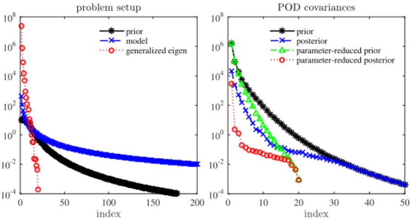
The left plot of Figure2 shows the spectra of the prior covariance matrixΓpr and of the system model L, along with the generalized eigenvalues (15) associated with the LIPS. The right plot of Figure2 compares the spectra of the state covariance matrices induced by the prior, the posterior, the parameter-reduced prior, and the parameter-reduced posterior. We see that the spectra of the covariance matrices induced by the prior and the posterior decay more slowly than the spectra induced by the parameter-reduced prior and parameter-reduced posterior. This difference is due to the high-dimensional complement prior, which induces state variations that are irrelevant to the observations. Projection onto the LIPS eliminates the effect of the complement prior, and thus the corresponding state covariance matrices have quickly decaying spectra that in fact vanish at index
20, which is the number of observations and the dimension of the LIPS. Note also that eigenvalues of the state covariance matrix induced by the parameter-reduced posterior decay more quickly than those induced by the parameter-reduced prior, since the posterior is more concentrated than the prior within the LIPS.
index 0 50 100 150 200 10-4 10-2 100 102 104 106 108 problem setup prior model generalized eigen index 0 10 20 30 40 50 10-4 10-2 100 102 104 106 108 POD covariances prior posterior parameter-reduced prior parameter-reduced posterior
Figure 2: The impact of parameter reference distributions on model reduction, as described in Example3.6. Left: spectra of the prior covariance matrix Γpr (stars) and the system model L(crosses), along with generalized
eigen-values from (15) (circles). Right: spectra of the state covariance matrices induced by the prior, the posterior, the parameter-reduced prior, and the parameter-reduced posterior; these are denoted by stars, crosses, triangles and circles, respectively.
Table 2: Summary of state reduction methods: the associated state covariance matrix, whether the process is offline/online, and whether adaptive sampling is required.
Method state covariance online/offline adaptive sampling?
Posterior-LISS Kfpost= R
Xu(Φrxr)u(Φrxr)
>π(dx
r|yobs) online yes
Laplace-LISS KfL =R Xu(Πrx)u(Πrx) >π L(dx) online no Prior-POD Kfpr =R Xu(Φrxr)u(Φrxr) >π 0(dxr) offline no
Since the amount of state variation in the reduced parameter subspace is greatly reduced relative to that induced by either the full-dimensional posterior or the full-dimensional prior, we will henceforth construct reduced-order models only within the reduced parameter subspace. For each state reduction technique of this kind, Table 2 summarizes the specific form of the state covariance, whether reduction is offline/online, and whether adaptive sampling is required, given the choice of parameter reference distribution. Overall, the benefit of pursuing model reduction on the reduced parameter subspace is twofold: first, this approach addresses challenges in the scalability of model reduction with parameter dimension; second, it reduces the computational cost of handling high-dimensional parameters in the parameterized reduced model.
3.2.3. Jointly-approximated posterior
By replacing the forward model F :Rn→Rd with the reduced-order model ˜F :Rr →Rd, the data-misfit function (4) can be approximated as
˜ η(xr) = 1 2k ˜ F(xr)−yobsk2Γobs. (28) Then the resultingjointly-reduced posterior distribution has the form
˜
π(xr|yobs)∝exp (−η˜(xr))π0(xr). (29)
Together with the complement prior, this defines a product-formjointly-approximated posterior
˜
π(x|yobs)∝π˜(xr, x⊥|yobs)∝π˜(xr|yobs)π0(x⊥). (30)
We use the descriptor ‘joint’ to signify that both the parameter space and the model state space have been reduced in these posterior approximations. Because the high-dimensional complement prior π0(x⊥) is analytically tractable and the low-dimensional jointly-reduced posterior avoids
computationally expensive full forward model evaluations, this jointly-approximated posterior can be used to design scalable and computationally efficient posterior exploration schemes.
Remark 3.7(Data reduction). In problems where the data set is high-dimensional, the computa-tion time required to evaluate the data-misfit funccomputa-tion (4) can also be significant. These evaluations can be accelerated by exploiting low-dimensional structure in the data space, via the DEIM method. Suppose that the dimension of the output of the observation model, y = C(Vsus,Φrxr), is much
larger than the reduced parameter dimension and the reduced state dimension. Suppose also that the variation of the model outputs,C(Vsus,Φrxr), can be captured by a subspace spanned by a basis
Yo ∈ Rd×o that is orthogonal with respect to h·,·iΓobs. As in the model reduction case, the DEIM
method can be used to identify a masking matrix Po = [δp1, . . . , δpo], where δi is the canonical
ba-sis in Ro, such that Po>Yo is nonsingular. Thus we can determine a low-dimensional coefficient function
β(us, xr) =Po>Yo−1Po>C(Vsus,Φrxr), (31)
which selectively evaluates the nonlinear function C at indices p1, . . . , po. The resulting
approxi-mated observation model has the form
˜
y=Yoβ(us, xr). (32)
In this setting, the coefficient function β and the reduced system model (20) together define a new reduced-order forward model Fˆ:Rr →Ro that has a smaller number of outputs. This corresponds
to model outputs y˜=YoFˆ(xr) in the original observable space. It leads to an approximated
data-misfit function in the form of
˜ η(xr) = 1 2 Yo ˆ F(xr)−yobs 2 Γobs = 1 2 ˆ F(xr)−Yo>Γ−1obsyobs 2 +c, (33)
where c= 12k(I −YoYo>)yobsk2Γobs is a constant. As in the state reduction case, we can also use a
POD approach with the reduced posterior, the Laplace approximation, or the parameter-reduced prior as reference distributions for constructing the parameter-reduced data basis.
3.3. Integrated algorithms
Concisely, construction of the jointly-approximated posterior distribution involves parameter reduction followed by model reduction. Combining the parameter reduction methods of Section
3.1 with the state reduction methods of Section3.2 leads to various integrated strategies for this task. We list several algorithmic options in Table3, distinguished according to their online/offline nature and whether adaptive sampling is required.
Table 3: Summary of sampling strategies for constructing the jointly-approximated posterior.
Strategy Prior-KL-POD Prior-Joint Laplace-Joint Posterior-Joint
Parameter reduction Prior-KL Prior-LIPS Laplace-LIPS Posterior-LIPS
State reduction Prior-POD Prior-POD Laplace-LISS Posterior-LISS
Sampling requirement offline offline online online and adaptive
3.3.1. Non-iterative strategies
The Prior-KL-POD strategy is the simplest option above: we compute the reduced parameter basis using the truncated KL expansion of the prior, and then compute a POD basis for the state by sampling from the parameter-reduced prior. In contrast, the Prior-Joint strategy uses the prior expectation of the GNH to construct a low-dimensional parameter subspace and defines the parameter-reduced prior accordingly; this strategy is still entirely offline, as both the parameter and state subspaces are independent of the data. Only prior samples are required in these two strategies. Full model evaluations in the Prior-POD step and Hessian evaluations in Prior-LIPS estimation can be massively parallelized. The computational cost of Prior-KL-POD is less than that of Prior-Joint, since the former involves no Hessians in the parameter reduction step.
Given observed data, the Laplace-Jointstrategy involves first finding the posterior mode by solving an optimization problem. Then samples can be directly drawn from the Laplace approxi-mation (12). In this way, the GNH evaluations required for Laplace-LIPS parameter reduction and the full model evaluations required for Laplace-LISS state reduction can also be carried out in par-allel. The computational cost thus is comparable to that of the Prior-Jointstrategy. However, in contrast withPrior-Joint,Laplace-Jointis an online strategy that depends on a particular realization of the observed data—and on the associated approximation of the posterior. Using the data focuses attention on regions of high posterior probability and leads to a localization effect in the identification of subspaces; thus, we expect that the jointly-approximated posterior com-puted by Laplace-Joint will have better accuracy than those produced by the Prior-KL-POD
orPrior-Joint strategies, for comparable dimensions of the parameter and state bases. We will explore this conjecture in numerical results below.
3.3.2. Iterative strategy
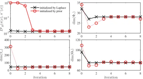
In thePosterior-Jointstrategy, constructing parameter and state subspaces requires comput-ing expectations over the full posterior (to obtain the posterior-LIPS) and the parameter-reduced posterior (to obtain the posterior-LISS). Since direct sampling is not feasiblea priori—after all, we are computing these bases in order tofacilitate posterior sampling—Algorithm1proposes an iter-ative sampling framework to construct the reduced bases adaptively during posterior exploration.
Algorithm 1 Iterative construction used in thePosterior-Jointstrategy. Require: At iteration k= 0, initialize the jointly-approximated posterior ˜π0(x|y
obs) to be either
the prior or the Laplace approximation (12).
Require: At iterationk, given (i) the reduced data-misfit function ˜ηk(xr) and the jointly-reduced
posterior ˜πk(xr|yobs) induced by the LIPS basis Φkr and the LISS basis Vsk; (ii) the
projec-tor Πkr = Φkr(Ξkr)> as in Definition 3.1; and (iii) the resulting jointly-approximated posterior ˜
πk(x|yobs), one iteration of the algorithm is: 1: if k= 0 then
2: Generate two sample sets,{xi}Ni=1 and {xi}Mi=1, from ˜π0(x|yobs) by direct sampling. 3: else
4: Generate two sample sets, {xi}Ni=1 and {xi}Mi=1, from ˜πk(x|yobs) by applying MCMC to
˜
πk(xr|yobs) and direct sampling to π0(x⊥). 5: end if
6: Compute the LIPS basis Φkr+1 by finding the dominant eigenvectors of (Sbpost,Γ−1pr), where
b Spost= 1 PN i=1ωi N X i=1 ωiH(xi), and ωi= exp ˜ ηk(Ξkr)>xi −η(xi) . (34)
7: Update the projector Πkr+1 = Φkr+1(Ξkr+1)> and compute the weighted snapshot matrix
U = q 1 PM i=1υi h√ υ1u Πkr+1x1 , . . . ,√υMu Πkr+1xM i , (35) where υi = exp ˜ ηk(Ξkr)>xi −η(Ξkr+1)>xi
, and then compute the reduced state basis
Vsk+1 via the SVD of U.
8: For system models involving nonlinear functions, compute the DEIM basis Θkt+1 as in Step 7, and then construct the masking matrixPtk+1.
9: Update ˜ηk+1(xr), ˜πk+1(xr|yobs) and ˜πk+1(x|yobs).
Note: At k= 0, importance sampling is turned off, i.e., ωi = 1 andυi = 1.
In Algorithm 1, we initialize the jointly-approximated posterior to be either the prior or the Laplace approximation (12). At each iteration k, two independent sets of samples are generated from the current jointly-approximated posterior, ˜πk(x|yobs), in order to construct reduced
param-eter and state bases using the Posterior-LIPS and Posterior-LISS methods, respectively. In this step, samples can be directly drawn when k = 0. For k > 0, sampling ˜πk(x|yobs) requires
ap-plying MCMC to the low-dimensional and cheap-to-evaluate jointly-reduced posterior ˜πk(xr|yobs),
and directly sampling the high-dimensional complement priorπ0(x⊥). At each iterationk, we use
the current jointly-approximated posterior ˜πk(x|yobs) as the biasing distribution to compute the
posterior expectation of the GNH via importance sampling; this process can be written as
Spost= Z X π(x|yobs) ˜ πk(x|y obs) H(x) ˜πk(dx|yobs). (36)
weight π(x|yobs) ˜ πk(x|y obs) ∝ω(x) := expη˜k(xr)−η(x) , where xr= (Ξkr) > x, (37)
can only be computed up to a normalizing constant. This leads to the self-normalized importance sampling estimator ofSbpostin (34). By finding the dominant eigenvectors of the pencil (Sbpost,Γ−1pr), we obtain the new LIPS basis Φkr+1.
Remark 3.8. We note that it is not feasible to store and factorize the matrix Sbpost directly. By
computing the action of the local GNHH(xi) on vectors—each action requires one forward model
evaluation and one adjoint model evaluation—low-rank approximations of each sampledH(xi) can
be computed using Krylov subspace methods [45] or randomized algorithms [46, 47]. Monte Carlo estimates of the expected Hessians used to identify the Laplace-LIPS and the Prior-LIPS are con-structed in the same way. We refer readers to [15, 17] for more details on storage management and computational strategies.
The updated LIPS basis Φkr+1 leads to a new parameter-reduced posterior πk+1(xr|yobs), and
then the next task is to compute the new reduced-order model using the Posterior-LISS. Since finding the Posterior-LISS requires integration over πk+1(xr|yobs), which can be computationally
expensive, we again employ importance sampling with the previous jointly-approximated posterior ˜
πk(x|yobs) as the biasing distribution. We use the following identity
f Kpost= Z Xr uΦkr+1xruΦkr+1xr>πk+1(dxr|yobs), = Z X uΠkr+1xuΠkr+1x>πˆk+1(dx|yobs),
to derive the importance sampling formula in the full parameter space. Thus, the state covariance estimated overπk+1(xr|yobs) can be written as
f Kpost= Z X ˆ πk+1(x|yobs) ˜ πk(x|y obs) uΠkr+1xuΠkr+1x> π˜k(dx|yobs). (38)
As in the parameter reduction case, the likelihood ratio ˆ πk+1(x|yobs) ˜ πk(x|y obs) ∝υ(x) := expη˜k(Ξkr)>x−η(Ξkr+1)>x, (39)
can only be computed up to a normalizing constant, and therefore we use self-normalized impor-tance sampling. When the SVD is used to compute the POD basis, this leads to the weighted snapshot matrix in (35). We note that the full model evaluation in the parameter-reduced data-misfit function η(Ξkr+1)>x in (39) generates exactly the snapshotu(Πkr+1x) used in computing the POD basis.
At the first iteration, the initial distribution ˜π0(x|yobs) can have a large discrepancy from
the posterior, and thus the resulting importance weights ωi and υi can potentially have large
variances. To overcome this potential sampling deficiency, we set the weightsωi and υi to 1 at the
first iteration. This way, the initial distribution is used as a surrogate to explore the support of the posterior, and importance sampling only kicks in at later iterations to estimate the LIPS and the LISS.
Remark 3.9. In each iteration of Algorithm 1, constructing the LIPS involves evaluating the forward model—and hence the full posterior density—at a set of samples, and computing the action of the GNH on a number of directions for each sample in this set. In addition, the forward model and the full posterior density are evaluated at another set of samples—projected onto the subspace spanned by the LIPS—to construct the reduced-order model. Based on our numerical experience, a sample size on the order of hundreds is sufficient for both steps. We also note that the first iteration of Algorithm1 generates a jointly-approximated posterior equivalent to the result of either the Prior-Joint strategy or the Laplace-Joint strategy, depending on the choice of initial distribution.
To ensure the convergence of the self-normalized importance sampling estimators (34) and (35), it is required that ˜πk(x|y
obs)>0 whenever π(x|yobs)>0 , and that ˜πk(x|yobs)>0 whenever
ˆ
πk+1(x|yobs)>0, for any k >0. Furthermore, distributions constructed from the low-dimensional
subspaces are not guaranteed to capture the tails of the posterior accurately, and hence the weights
ω(x) andυ(x) might have large variance in some situations. Boundingω(x) andυ(x) from above, however, can control the variance of the importance weights and thus guarantee finite variance of the estimators. The following lemma establishes that by assigning upper bounds to the approximated data-misfit functions, the ratiosω(x) and υ(x) can be bounded.
Lemma 3.10. Given an upper bound K >0 on the parameter-approximated data-misfit function
η(Ξ>rx) and the jointly-approximated data-misfit function η˜(Ξ>rx), i.e.,
η(Ξ>rx)≤K <∞ and ˜η(Ξ>rx)≤K <∞, (40)
the ratios ω(x) and υ(x) defined in (36) and (39) are bounded as ω(x) ≤ exp(K) and υ(x) ≤ exp(K).
Proof. Since all the data-misfit functions have the form of a weightedL2 norm, their values cannot be negative, i.e., η(x) ≥ 0, η(Ξ>rx) ≥ 0, and ˜η(Ξ>rx) ≥ 0. The upper bounds on η(Ξ>rx) and ˜ η(Ξ>rx) in (40) then lead to ˜ η(xr)−η(x)≤K and ˜η(Ξ>rx)−η(Ξ > rx)≤K.
Thus both ratiosω(x) and υ(x) are bounded above by exp(K).
We employ a heuristic based on a (somewhat frequentist) probabilistic argument to choose a value ofKto impose as a bound on our misfit functions. If the whitened residual in the data-misfit function, Γ−1obs/2(F(x)−yobs), is ad-dimensional random vector whose components are independent
standard Gaussians, then the data-misfit function follows a chi-squared distribution withddegrees of freedom,χ2d. Then the upper boundK can be chosen so that the probability of the data-misfit function exceedingK is τd1, i.e.,
P[z > K] =τd, where z∼χ2d.