https://doi.org/10.1007/s13675-019-00114-8
O R I G I N A L P A P E R
Bilevel programming methods for computing
single-leader-multi-follower equilibria in normal-form and
polymatrix games
Nicola Basilico1 ·Stefano Coniglio2 ·Nicola Gatti3 ·Alberto Marchesi3
Received: 3 October 2018 / Accepted: 10 May 2019 © The Author(s) 2019
Abstract
The concept of leader-follower (or Stackelberg) equilibrium plays a central role in a number of real-world applications bordering on mathematical optimization and game theory. While the single-follower case has been investigated since the inception of bilevel programming with the seminal work of von Stackelberg, results for the case with multiple followers are only sporadic and not many computationally affordable methods are available. In this work, we consider Stackelberg games with two or more followers who play a (pure or mixed) Nash equilibrium once the leader has committed to a (pure or mixed) strategy, focusing on normal-form and polymatrix games. As cus-tomary in bilevel programming, we address the two extreme cases where, if the leader’s commitment originates more Nash equilibria in the followers’ game, one which either maximizes (optimistic case) or minimizes (pessimistic case) the leader’s utility is selected. First, we show that, in both cases and when assuming mixed strategies, the optimization problem associated with the search problem of finding a Stackelberg equilibrium isN P-hard and not in Poly-APX unlessP = N P. We then consider different situations based on whether the leader or the followers can play mixed strate-gies or are restricted to pure stratestrate-gies only, proposing exact nonconvex mathematical programming formulations for the optimistic case for normal-form and polymatrix games. For the pessimistic problem, which cannot be tackled with a (single-level) mathematical programming formulation, we propose a heuristic black-box algorithm. All the methods and formulations that we propose are thoroughly evaluated compu-tationally.
Keywords Bilevel programming·Game theory·Stackelberg games·Equilibrium computation
Mathematics Subject Classification 91A10·91A65·91A90·90C26
1 Introduction
Leader-follower(orStackelberg)gamesmodel the interaction between rational agents (or players) when a hierarchical decision-making structure is in place. Considering, for simplicity, the two-player case, Stackelberg games model situations where an agent (theleader) plays first and a second agent (thefollower) plays right after them, after observing the strategy the leader has chosen.
The number of real-world problems where a leader-follower (or Stackelberg) struc-ture can be identified is extremely large. This is often the case in the security domain (An et al.2011; Kiekintveld et al.2009), where a defender, aiming to protect a set of valuable targets from the attackers, plays first, while the attackers, acting as followers, make their move only after observing the leader’s defensive strategy. Other notewor-thy cases are interdiction problems (Caprara et al.2016; Matuschke et al.2017), toll setting problems (Labbé and Violin2016), network routing problems (Amaldi et al.
2013) and (singleton) congestion games (Castiglioni et al.2018; Marchesi et al.2018). While, since the seminal work of von Stackelberg (2010), the case with a single leader and a single follower has been widely investigated, only a few results are known for the case with multiple followers and not many computationally affordable methods are available to solve the corresponding equilibrium-finding problem.
In this paper, we focus on the fundamental case of single-leader multi-follower games with a finite number of actions per player where the overall game can be represented as a normal-form or polymatrix game—the latter is of interest as it plays an important role in a number of applications such as in the security domain, where the defender may need to optimize against multiple uncoordinated attackers solely interested in damaging the leader. Throughout the paper, we assume the setting where the (two or more) followers play simultaneously in a noncooperative way, for which it is natural to assume that, after observing the leader’s play (either as a strategy or as an action), the followers would reach aNash equilibrium(NE) (see Shoham and Leyton-Brown (2008) for a thorough exposition of this equilibrium concept). We refer to an equilibrium in such games asleader-follower Nash equilibrium(LFNE).
As it is typical in bilevel programming, we study two extreme cases: the optimistic one where, if the leader’s commitment originates more NE in the followers’ game, one which maximizes the leader’s utility is selected, and the pessimistic one where an equilibrium which minimizes the leader’s utility is chosen.
In particular, the leader’s utility at an optimistic equilibrium corresponds to the largest utility the leader may get assuming the best case in which the followers would (somehow) end up playing a Nash equilibrium which maximizes the leader’s utility. Differently, the leader’s utility at a pessimistic equilibrium corresponds to a utility value the leader could always get independently of the followers’ behavior. From this perspective, a risk-taking leader would play according to an optimistic equilibrium, whereas a risk-averse leader would play according to a pessimistic equilibrium. For more types of solution concepts related to these two, we refer the reader to Alves and Antunes (2016).
The original contributions of our work are as follows.1First, we illustrate that the optimization problem associated with the search problem of computing an LFNE in mixed strategies when the followers play an NE which either maximizes or minimizes the leader’s utility isN P-hard and not in Poly-APX unlessP =N P. After casting the general problem with mixed-strategy commitments in bilevel terms, we propose different nonlinear and nonconvex single-level mathematical programming formu-lations for the optimistic case, suitable for state-of-the-art spatial-branch-and-bound solvers. For the pessimistic case, which does not admit a single-level mathematical programming reformulation of polynomial size, we propose a heuristic method based on the combination of a spatial-branch-and-bound solver with ablack-boxalgorithm. We also briefly investigate (easier) variants of the problem obtained when restricting either the leader or the followers to pure-strategy commitments. We conclude by pro-viding a thorough experimental evaluation of our techniques on a (normal-form and polymatrix) test bed generated with GAMUT (Nudelman et al.2004), also encom-passing some structured games, employing different solvers: BARON, SCIP, CPLEX, SNOPT and RBFOpt. (The latter is used for black-box optimization).
2 Notation
LetN = {1, . . . ,n}be the set of agents. For eachp∈ N, we denote byApthe agent’s set of actions, withmp= |Ap|. For each agent p ∈ N, we denote byxp ∈ [0,1]mp, witheTxp =1 (whereeis the all-one vector), theirstrategy vector(or strategy, for short). Each componentxapof xprepresents the probability by which agent p plays actiona ∈ Ap. We callxpa vector ofpure strategiesifxp ∈ {0,1}mp or ofmixed strategiesin the general case. We denote astrategy profile, i.e., the collection of the strategies each agent plays, byx =(x1, . . . ,xn).
For each agent p ∈ N, we define their utility function asup : [0,1]m1 × · · · ×
[0,1]mn → R. A strategy profilex =(x
1, . . . ,xn)is an NE if and only if, for each agent p ∈ N,up(x1, . . . ,xn)≥ up(x1, . . . ,xn)for every strategy profilex where xq = xq for allq ∈ N\{p}andxp = xp. (This corresponds to assuming that no unilateral deviations would take place.) We consider two game classes:normal-form
(NF) andpolymatrix(PM).
For NF games (see Shoham and Leyton-Brown (2008) for a reference), we let
Up ∈ Rm1×···×mn denote, for each agent p ∈ N, their (multi-dimensional) utility (or payoff) matrix where each component Ua1,...,an
p denotes the utility of agent p when all the agents play actionsa1, . . . ,an. Given a strategy profile(x1, . . . ,xn), the expected utility of agentp ∈Nis equal to the multi-linear functionup(x1, . . . ,xn)= xTp(Up·
q∈N\{p}xq).
For PM games (see Yanovskaya (1968) for a reference), we have a utility matrix
Upq ∈ Rmp×mq per pair of agents p,q ∈ A. Given a strategy profile(x1, . . . ,xn), the expected utility of agent p is equal to the bilinear function up(x1, . . . ,xn) =
q∈N\{p}xTpUpqxq.
1 Some parts of the paper were presented at a preliminary stage in Basilico et al. (2016) and Basilico et al.
We remark that, while in the NF case the degree of the polynomial corresponding to an agent’s expected utility is equal to the number of agents, it is always equal to 2 in the PM case, independently of the number of agents involved. The computational impact of this property will be discussed in the paper.
3 Previous works
Since the original work of Nash (1950), the problem of computing Nash equilibria in multi-player games (without a leader) has attracted a large interest—see the monograph (von Stengel2010and Chen and Deng2006; Conitzer and Sandholm2008) where the complexity of the problem is addressed. For more details on noncooperative game theory, we refer the interested reader to Shoham and Leyton-Brown (2008).
Most of the game-theoretic investigations on Stackelberg games have, to the best of our knowledge, mainly addressed the case of a single follower. In such setting, it is known that the single follower can play a pure strategy without loss of generality, i.e., that there always is a pure strategy by which they can maximize their utility and that the optimization problem associated with the search problem of computing an equilibrium is easy with complete information (von Stengel and Zamir2010), while it becomesN P-hard for Bayesian games (Conitzer and Sandholm2006). Algorithms are proposed in Conitzer and Sandholm (2006).
For what concerns Stackelberg games with more than two players, some works have investigated the case with multiple leaders and a single follower; see Leyffer and Munson (2010). For the problem involving a single leader and multiple followers (the one on which we focus in this paper), only a few results are available. It is known, for instance, that an equilibrium can be found in polynomial time if the followers play a correlated equilibrium in the optimistic case (Conitzer and Korzhyk2011) (see Shoham and Leyton-Brown2008for more detail on correlated equilibria), whereas the associated optimization problem isN P-hard if they play sequentially one at a time (as in a classical Stackelberg game with many players) (Conitzer and Sandholm
2006).
4 Problem statements, bilevel perspective and computational
complexity
In this section, we formalize the problem that we address in the paper, cast it in bilevel terms and investigate its computational complexity and approximability.
4.1 Problem statements
In formal terms, the two main versions of the problem of computing an LFNE that we tackle in this paper, optimistic (O-LFNE) and pessimistic (P-LFNE), are defined as follows:
O-LFNE: Given ann-agent game withn ≥ 3, find a strategy vectorδ for the leader such that, after committing, the largest leader’s utility over all the NE in the followers’ game parameterized byδis as large as possible.
P-LFNE: Given ann-agent game withn ≥ 3, find a strategy vectorδ for the
leader such that, after committing, the smallest leader’s utility over all the NE in the followers’ game parameterized byδis as large as possible.
When notationally convenient, we will refer to an either optimistic or pessimistic LFNE as O/P-LFNE.
We will distinguish between the cases where either the leader or the followers are restricted or not to pure strategies, considering four cases: leader in mixed and followers in mixed (LMFM), leader in pure and followers in mixed (LPFM), leader in mixed and followers in pure (LMFP), and leader in pure and followers in pure (LPFP). In the general (mixed) case, we assume that the leader commits to a strategy, i.e., to a distribution of probability according to which they (the leader) select their action, and that, while the followers can observe the distribution chosen by the leader, they (the followers) cannot observe its realization (i.e., the action the leader plays). This is the case in, e.g., security games. The case in which the leader’s strategy is pure is the converse one in which the leader’s play is completely observable by the followers. The assumption behind the followers playing mixed strategies is the same as in games without a leader (e.g., one can consider repeated games in which the leader has to commit to a single strategy before the game starts, whereas the followers can, at each iteration, draw a different action profile from their distribution of choice, thus playing mixed strategies).
For the sake of presentation, in the remainder of the paper we assumen =3 (one leader, two followers). We remark that our results can be adapted to anyn. In Sect.9, we will indeed report on computational experiments carried out for games with more than two followers.
In the remainder of the paper, we assume that the last agent (the third), whom we relabel as agent, takes the role of leader. All the other agents (the followers) are compactly denoted by the setF = N\{}. Whenn =3,F = {1,2}. For all f ∈ F, we define f:=F\{f}. We also denotex(the strategy vector of the leader) byδand
x1,x2(the strategy vectors of the followers) byρ1, ρ2. For each p ∈ N, we letΔp be thesimplex of strategiesof player p, i.e., the set of nonnegative vectorsδ,ρ1orρ2
summing to 1.
4.2 Bilevel programming perspective
Computing an O/P-LFNE amounts to solving abilevel programming problem. In the optimistic case, we can compute an O-LFNE by solving the following prob-lem: (O-LFNE) max (ρ1,ρ2,δ)∈ Δ1×Δ2×Δ i∈A1 j∈A2 k∈A Ui j kρ1iρ j 2δ k (1a)
s.t. ρ1∈argmax ρ1∈Δ1 i∈A 1 j∈A2 k∈A U1i j kρ1iρ2jδk (1b) ρ2∈argmax ρ2∈Δ2 i∈A 1 j∈A2 k∈A U2i j kρ1iρ2jδk . (1c)
Due to Constraints (1b)–(1c), the second-level problems call for a pair(ρ1, ρ2)of
followers’ strategies forming an NE in the followers’ game induced by the strategy
δ∈Δchosen by the leader in the first level. Note that, due to the definition of NE, the pair(ρ1, ρ2)is an NE in the game induced byδif and only ifρ1(resp.,ρ2) maximizes
player 1’s (resp., player 2’s) utility when assuming that player 2 (resp., player 1) plays
ρ2(resp.,ρ1). Subject to these constraints, the first level calls for a triple(ρ1, ρ2, δ)
maximizing the leader’s utility.
The problem is optimistic as, assuming that the second level admits many NE
(ρ1, ρ2)for the chosenδ, it calls for a pair(ρ1, ρ2)which, together withδ, maximizes
the leader’s utility. Notice that, while any triple(ρ1, ρ2, δ)∈Δ1×Δ2×Δis afeasible
solution to the problem as long as the pair(ρ1, ρ2)is an NE in the game induced byδ,
Problem (1a)–(1c) calls for a triple(ρ1, ρ2, δ)which isoptimal—as, if not, the leader
would prefer to change their strategy and(ρ1, ρ2, δ)would not be a LFNE.
In the pessimistic case, computing a P-LFNE amounts to solving to the following problem: (P-LFNE) max δ∈Δ(ρmin1,ρ2)∈ Δ1×Δ2 i∈A1 j∈A2 k∈A Ui j kρ1iρ2jδk (2a) s.t. Constraints (1b), (1c). (2b) This problem differs from its optimistic counterpart as, due to the assumption of pessimism, the leader here maximizes theminimumvalue taken by their utility over all pairs(ρ1, ρ2)which are NE in the followers’ game induced byδ—that is, for the
chosenδ,ρ1andρ2always correspond to a NE which minimizes the leader’s utility.
4.3 Complexity results
As we will show, the optimization problem associated with the search problem of computing an LFNE is bothN P-hard and inapproximable in both versions (O-LFNE and P-LFNE) in the LMFM case even with a single leader action (which implies that the result also holds for the LPFM case). This follows from theN P-hardness and inapproximability of the problem of computing, in a two-player game, a mixed-strategy NE which maximizes the sum of the players’ utilities (the so-calledsocial welfare) (Conitzer and Sandholm2008):
Proposition 1 (Conitzer and Sandholm2008) The problem of computing a mixed-strategy NE which maximizes the total players’ utility isN P-hard and it is not in
The result is based on the fact that, for any SAT instance, it is possible to build a symmetric two-player game(U1,U2), either NF or PM, such that:
(i) there is a (pure-strategy) NE in which both players play their last action and receive a utility equal to >0, whereis an arbitrarily small constant;
(ii) the game admits a (mixed-strategy) NE providing each player with a utility ofm, wheremis the number of actions, if and only if the SAT instance is a YES instance. This implies that, in any such game, finding an NE where the players achieve a utility strictly larger thanwould suffice to claim that the corresponding SAT instance is a YES instance. It follows that one cannot decide in polynomial time whether such games admit an NE providing the players with a utility strictly larger thanunlessP =N P as, if that were the case, YES instances of SAT could be decided in polynomial time. This also shows that finding an NE which maximizes the social welfare (defined as the total players’ utility) is not inAPX. This is because the existence of an NE providing the players with a total utility strictly greater than 2would suffice to conclude that the corresponding SAT instance admits answer YES.
We show that the result in Conitzer and Sandholm (2008) can be strengthened with a simple observation:
Proposition 2 The problem of computing a mixed-strategy NE which maximizes the total players’ utility is not in Poly-APX unlessP = N P, even when the game is polymatrix.
Proof Let= 21m. On games corresponding to YES SAT instances (which admit an
NE with total utility 2m), an algorithm with approximation ratio α1 would yield an NE of total utility at least 1α2m. Note that, if 1α2m > 2(i.e., α1 > m), the SAT instance is proved to be a YES instance. Therefore, there cannot be a polynomial time approximation algorithm with a factor better than m = 2m1m unlessP =N P. Since
the reciprocal of this factor is superpolynomial, the problem is not in Poly-APX. For the problem of computing an O/P-LFNE, we show the following result:
Proposition 3 The optimization problem associated with the search problem of com-puting an O/P-LFNE in the LMFM and LPFM cases is N P-hard and it is not in Poly-APX unlessP=N P, even when the game is polymatrix.
Proof Let us consider the O-LFNE case first. Given a game with utilities(U1,U2)
andmactions per player as defined in Conitzer and Sandholm (2008), we construct a 3-player leader-follower polymatrix game where:
– the leader only has one action and utility matricesUf1 =Uf2 =
1, . . . ,1,21m
; – player f1’s utility matrices areUf1 =0andUf1f2 =U1;
– player f2’s utility matrices areUf2=0andUf2f1 =U2.
Due to having a single action, the presence of the leader is immaterial. (Note that, therefore, the LMFM and LPFM cases coincide.) Therefore, the set of followers’ equilibria in the leader-follower game is the same as that of the original two-player game. It follows that SAT has answer YES if and only if the leader-follower game admits an equilibrium with leader’s utility strictly larger than 21m, as that corresponds
to an NE in the followers’ game with utility strictly larger thanfor each player. Along the lines of the previous proof, an algorithm with approximation factorα1would yield, for a YES instance, a leader utility of at least α1, allowing us to conclude that the instance is a YES instance if α1 > 21m. This shows that the problem of computing an
O-LFNE is not in Poly-APX unlessP =N P(even in polymatrix games).
For the computation of a P-LFNE, the reasoning is the same except for defining
Uf1 =Uf2 =
1
2m,21m, . . . ,21m,1
.
We conclude the section by showing that deciding whether one of the leader’s actions can be safely discarded is a hard problem, which implies that dominance-like techniques often used in game theory to reduce the search space of an equilibrium-computing algorithm are inapplicable.
Proposition 4 In the LMFM case, deciding whether an action of the leader is played with strictly positive probability at an O/P-LFNE isN P-hard.
Proof Given a symmetric two-player game (U1,U2) withm actions as defined in
Conitzer and Sandholm (2008), we build a three-player game(U,Uf1,Uf2)in which:
– the leader has two actions, while f1and f2havemactions each;
– when the leader plays their first action, the payoffs of all the players are 1/4; – when the leader plays their second action, the payoffs of f1and f2 are those in
(U1,U2)and the leader’s payoffs are 1 for all the actions of f1and f2, except for
the combination composed of the last action of f1and the last action of f2, in
which the leader’s payoff is 0.
We show that the first action of the leader can be safely discarded from the game
(U,Uf1,Uf2)if and only if the game(U1,U2)admits a mixed-strategy NE providing
the players with a utility ofm, which implies that deciding whether the first action of the leader can be discarded isN P-hard. If the leader plays their first action, they receive a utility of 1/4. If the leader plays their second action, the followers play the best NE for the leader, which can be either (i) the pure-strategy NE in which both play their last action providing the leader with a utility of 0 or (ii) if it exists, the mixed-strategy NE providing the leader with a utility of 1. For any mixed strategy of the leader, the behavior of the followers does not change w.r.t. the case in which the leader plays their second action as a pure strategy. This is because, when the leader randomizes between their two actions, the utility of the followers f1 and f2 is an
affine transformation (with positive coefficients) of U1 andU2, making them play
exactly as in the case where the leader plays their second action as a pure strategy. Thus, at an optimistic LFNE the leader plays a pure strategy, playing their first action if(U1,U2)does not admit a mixed-strategy NE and their second action if it does.
The first action of the leader can therefore be safely discarded if and only if(U1,U2)
admits a mixed-strategy NE providing the players with a utility ofm.
The proof is analogous in the pessimistic case after interchanging the leader payoffs
5 Optimistic case with leader in mixed and followers in mixed
(O-LMFM)
In this section, we focus on the optimistic setting in the general case where each player is allowed to play mixed strategies. We propose three different exact mathematical programming formulations for NF games and then illustrate how they can be simplified for PM games.
5.1 Exact formulations for NF games
We report the three formulations illustrating how to derive each of them in sequence.
5.1.1 O-NF-LMFM-I
To obtain a single-level formulation for the problem, we proceed by applying a stan-dard reformulation (Shoham and Leyton-Brown 2008) involving complementarity constraints.
Let, for alli ∈ A1andj ∈ A2,U˜1i j :=
k∈AU i j k 1 δ kandU˜i j 2 = k∈AU i j k 2 δ kbe the matrices of the followers’ game, parameterized byδ. According to Constraint (1b), for(ρ1, ρ2)to be a NEρ1must be an optimal solution to the Linear Program (LP):
max ρ1∈Δ1 i∈A1 j∈A2 ˜ U1i jρ1iρ2j ,
whereU˜1i jρ1iρ2j is a linear function ofρ1ifρ2is fixed. Since the LP is feasible and
bounded for anyρ2 ∈ Δ2, by complementary slackness we have that ρ1 ∈ Δ1 is
optimal if and only if there is a scalarv1such that the following holds for alli ∈ A1:
v1− j∈A2U˜ i j 1 ρ j 2 ρi 1=0 v1≥ j∈A2U˜ i j 1ρ j 2.
v1 can be interpreted as thebest-response valueof follower 1, equal to the largest
utility the follower can achieve at an equilibrium. Applying a similar reasoning toρ2,
we obtain thatρ2 ∈ Δ2 is optimal if and only if there is a scalarv2 such that the
following holds for all j ∈ A2:
v2− i∈A1U˜ i j 2 ρ1i ρj 2 =0 v2≥ i∈A1U˜ i j 2 ρ i 1.
We conclude that(ρ1, ρ2)is an NE if and only if there arev1, v2≥0 such thatρ1and
After substituting forU˜1andU˜2their linear expressions inδ, we obtain the following
constraints for player 1 and for alli ∈ A1:
v1− j∈A2 k∈AU i j k 1 ρ j 2δk ρi 1=0 v1≥j∈A2k∈AU1i j kρ2jδk.
For player 2 and for all j ∈ A2, we obtain:
v2− i∈A1 k∈AU i j k 2 ρ1iδk ρj 2 =0 v2≥ i∈A1 k∈A U2i j kρ1iδk.
By imposing such constraintsin lieuof the two second-level argmax constraints of Problem (1) (Constraints (1b)–(1c)), we obtain a continuous single-level formulation with nonconvex trilinear terms.2Overall, the formulation reads:
max ρ1,ρ2,δ,v i∈A1 j∈A2 k∈A Ui j kρ1iρ2jδk (3) s.t. v1− j∈A2 k∈A U1i j kρ2jδk ρi 1=0 ∀i ∈ A1 (4) v1≥ j∈A2 k∈A U1i j kρ2jδk ∀i ∈ A1 (5) v2− i∈A1 k∈A U2i j kρi1δk ρj 2 =0 ∀j ∈ A2 (6) v2≥ i∈A1 k∈A U2i j kρ1iδk ∀j ∈ A2 (7) k∈A δk=1, δ≥0 (8) i∈Af ρi f =1, ρf ≥0 ∀f ∈ F (9) vf ≥0 f ∈F. (10)
The problem containsm1+m2cubic constraints,m1+m2quadratic constraints and
a cubic objective function.
2 Note that strong duality can be employed in place of complementary slackness. Preliminary experiments
5.1.2 O-NF-LMFM-II
What we propose now is aimed at achieving a formulation which can be solved more efficiently. Since each term of the complementarity constraints we introduced is bounded from above and below, we can apply a simple reformulation along the lines of Sandholm et al. (2005). Lets1∈ {0,1}m1ands2∈ {0,1}m2 be theantisupport vectors
ofρ1andρ2, (i.e., two binary vectors withm1and, respectively,m2components each
of which has value 0 if and only ifρ1and, respectively,ρ2is strictly positive in that
component). It suffices to impose the following constraints for alli ∈ A1:
ρi 1≤1−s1i v1− j∈A2 k∈A U1i j kρ2jδk≤ Ms1i
and the following ones for all j ∈ A2:
ρj 2 ≤1−s j 2 v2− i∈A1 k∈A U2i j kρi1δk ≤Ms2j.
M is an upper bound on the entries of U1,U2. This way, while still retaining the
original trilinear objective function only bilinear constraints are needed. We obtain the following reformulation:
max ρ1,ρ2,δ,v,s i∈A1 j∈A2 k∈A Ui j kρi1ρ j 2δ k (11) s.t. v1− j∈A2 k∈A U1i j kρ2jδk≤ Ms1i ∀i ∈ A1 (12) v2− i∈A1 k∈A U2i j kρ1iδk ≤Ms2j ∀j∈ A2 (13) ρi f ≤1−s i f ∀f ∈F,i ∈ Af (14) sjf ∈ {0,1} ∀f ∈F,j ∈ Af (15) Constraints (5), (7), (8)–(10). (16) At the cost of introducing binary variables, with this formulation we achieve fewer nonlinearities: only 2m1+2m2quadratic constraints and a cubic objective function. 5.1.3 O-NF-LMFM-III
Ultimately, we aim to solve the problem with spatial-branch-and-bound techniques, such as those implemented in BARON and SCIP. The main strategy of such methods
to handle nonlinearities is to isolate “simple” nonlinear terms (bilinear or trilinear in our case) by shifting them into a new (so-calleddefining) constraint to which a convex envelope is applied.
We propose to anticipate this reformulation, so to be able to derive some valid constraints. First, we introduce:
(i) variabley2j k and constrainty2j k =ρ2jδkfor all j ∈ A2,k∈ A,
(ii) variabley1i k and constrainty1i k =ρ1iδk for alli ∈ A1,k∈ A,
(iii) variablezi j kand constraintzi j k =ρ1iy2j k for alli∈ A1,j ∈ A2,k∈ A.
By substituting each bilinear and trilinear term with the newly introduced variables, we then obtain a formulation which is linear everywhere, except for the defining constraints themselves.
The advantage of carrying out this reformulation stepa prioriis that we can now observe that, after introducing the new variables, the matrix {y2j k}j k∈A2×A is, by
definition, the outer product of the stochastic vectors ρ2 and δ and, as such, is a
stochastic matrix itself. The same holds for the tensor{zi j k}i j k∈A1×A2×A, which is
the outer product of the vectors ρ1, ρ2, δ and, as such, is a stochastic tensor. This
implies the validity of the following three constraints:
i∈A1 k∈A y1i k =1 j∈A2 k∈A y2j k =1 i∈A1 j∈A2 k∈A zi j k =1.
We remark that these inequalities are a subset of those that are obtained by applying a relaxation-linearization techniqueà laSherali and Adams (1990) to Constraints (8) and (9).
The formulation that we obtain is the following one: max ρ1,ρ2,δ,v,s,y,z i∈A1 j∈A2 k∈A Ui j kzi j k (17) s.t. v1≥ j∈A2 k∈A U1i j ky2j k ∀i∈ A1 (18) v2≥ i∈A1 k∈A U2i j ky1i j ∀j∈ A2 (19) v1− j∈A2 k∈A U1i j ky2j k ≤Msi1 ∀i ∈ A1 (20) v2− i∈A1 k∈A U2i j ky1i k ≤Ms j 2 ∀j ∈ A2 (21) yi kf =ρifδk ∀k∈ A, f ∈ F,i ∈ Af (22)
zi j k =ρ1iy2j k k∈ A,i ∈ A1,j ∈ A2 (23) i∈Af k∈A yi kf =1 ∀f ∈F (24) i∈A1 j∈A2 k∈A zi j k =1 (25) yi jf ≥0 ∀f ∈ F,i ∈ Af,k∈ A (26) zi j k ≥0 ∀i∈ A1,j ∈ A2,k∈ A (27) Constraints(8)–(10),(14)–(15). (28) Overall, we obtainm(m1+m2)+mm1m2 quadratic constraints and a linear
objective function, yielding a tighter formulation than O-NF-LMFM-II, as we will show computationally.
5.2 Exact formulations for PM games
We illustrate how the three formulations we proposed can be substantially simplified for PM games.
5.2.1 O-PM-LMFM-I
In PM games, the expected utility for follower 1 corresponding to an actioni ∈ A1
(which is a trilinear function for NF games withn =3 and of ordernin general) is defined as the following linear function (which is linear for anynand, in particular, forn =3): k∈A U1i kδk+ j∈A2 U12i jρ2j.
The leader’s utility is the following function, bilinear for anyn:
k∈A i∈A1 Ui k1ρ1iδk+ k∈A j∈A2 Uj k2ρ2jδk.
As a consequence, the PM counterpart to formulation O-NF-LMFM-I reads: max ρ1,ρ2,δ,v k∈A i∈A1 Ui k1ρ1iδk+ k∈A j∈A2 Uj k2ρ2jδk (29) s.t. v1≥ k∈A U1i kδk+ j∈A2 U12i jρ2j ∀i∈ A1 (30) v2≥ k∈A U2j kδk+ i∈A1 U21i jρ1i ∀j ∈ A2 (31)
v1− k∈A U1i kδk+ j∈A2 U12i jρ2j ρi 1=0 ∀i∈ A1 (32) v2− k∈A U2j kδk+ i∈A1 U21i jρ1i ρj 2 =0 ∀j ∈ A2 (33) Constraints(8)–(10. (34) Differently from the NF case, this formulation only containsm1+m2quadratic
constraints and a quadratic objective (as Constraints (5) and (7) become linear here, while Constraints (4) and (6) and Objective (3) become quadratic).
5.2.2 O-PM-LMFM-II
Applying for the PM case the same reformulation we carried out in O-NF-LMFM-II, we obtain: max ρ1,ρ2,δ,v,s k∈A i∈A1 Ui k1ρ1iδk+ k∈A j∈A2 Uj k2ρ2jδk (35) s.t. v1− k∈A U1i kδk+ j∈A2 U12i jρ2j ≤ Ms1i ∀i ∈ A1 (36) v2− k∈A U2j kδk+ i∈A1 U21i jρ1i ≤Ms2j ∀j∈ A2 (37) Constraints (8)–(10),(14)–(15),(30)–(31). (38) Besides the binary variables, this formulation contains only linear constraints and a quadratic objective.
5.2.3 O-PM-LMFM-III
Similarly to O-NF-LMFM-III, this formulation is derived by reformulating each multi-linear term in O-PM-LMFM-II. In the latter, the only nonmulti-linearity is in the objective function. Therefore, O-PM-LMFM-III is obtained by just reformulating the products
δiρj
f it contains for all f ∈ Fandj ∈ Af, adding valid constraints identical to those we added to O-NF-LMFM-III. We obtain:
max ρ1,ρ2,δ,v,s,y k∈A i∈A1 Ui k1yi k1 + k∈A j∈A2 Uj k2y2j k (39) s.t. Constraints (8)–(10),(14)–(15),(22),(24),(26),(30)–(31),(36)–(37). (40) Similarly to O-NF-LMFM-III, O-PM-LMFM-III is completely linear except for them(m1+m2)defining quadratic Constraints (22).
6 Pessimistic case with leader in mixed and followers in mixed
(P-LMFM)
UnlessP =N P, it is clear that there is no single-level formulation of polynomial size (in terms of variables and constraints) for the problem of computing a pessimistic LFNE. This is because, given a tripleδ, ρ1, ρ2, a single-level reformulation of
poly-nomial size for the problem would allow for checking whether, for the givenδ, the
(ρ1, ρ2)pair yields not just an NE (this can be checked in polynomial time by
inspect-ing polynomially many constraints) but anoptimal one. That is, it would allow us to verifyin polynomial timewhether a given solution to anN P-hard problem is optimal, which cannot be done in general unlessP =N P.
For this reason, we adopt a different approach here, designing a heuristic method to tackle the pessimistic case based on a black-box solver coupled with an exact oracle. While the method is conceived to tackle the pessimistic case, it can also be used for the optimistic one (as we show in Computational results section).
The method is based on a radial basis function (RBF) estimation which relies on the solver RBFOpt (Costa et al.2015). The idea is of exploring the leader’s strategy space (variablesδ) with a direct search which iteratively builds an RBF approximation of the objective function relying on the solution of anoracle formulationwhich is responsible for carrying out the objective function evaluation.
Given any incumbent valueδˆ, the oracle solves the (NF or PM) second-level problem exactly after imposingδ= ˆδ. For NF games, the oracle formulation we use is similar to O-NF-LMFM-III, employing a different reformulation with auxiliary variablesyj k= ρj
1ρ2k, which yields a tighter reformulation than the original one in O-NF-LMFM-III
whenδis given (as in this case). Crucially, in this formulation the sign of the objective function has to be changed so to produce a pair(ρ1, ρ2)which minimizes the leader’s
objective function (rather than maximizing it) for the givenδ= ˆδ.
The oracle formulation for the optimistic and pessimistic cases reads as follows (± indicates that the sign of the objective function has to be flipped from+to−in the pessimistic case): max ρ1,ρ2,v,s,y ± i∈A1 j∈A2 k∈A Ui j kyi jδˆk (41) s.t. v1≥ j∈A2 k∈A U1i j kρ2jδˆk ∀i ∈ A1 (42) v2≥ i∈A1 k∈A U2i j kρi1δˆk ∀j ∈ A2 (43) v1− j∈A2 k∈A U1i j kρ2jδˆk ≤Msi1 ∀i∈ A1 (44) v2− i∈A1 k∈A U2i j kρ1iδˆk≤ Ms2j ∀j ∈ A2 (45) yi j =ρ1iρ2j ∀i∈ A1,j ∈ A2 (46)
i∈A1 j∈A2 yi j =1 (47) yi jf ≥0 ∀f ∈ F,i ∈ Af,k∈ A (48) Constraints (8)–(10),(14)–(15). (49) Besides the defining constraints for yi j, the other parts of the formulation are all linear.
For PM games, we can directly use formulation O-PM-LMFM-II: Since each of the nonlinear terms in O-PM-LMFM-II is bilinear and it involvesδ, whenδis fixed toδˆthe formulation corresponds to a mixed-integer linear program (MILP).
7 Optimistic case with leader in pure and followers in mixed (O-LPFM)
We focus now on the case in which the leader is restricted to pure strategies.7.1 Exact formulations for NF and PF games
As it is clear, in the LPFM case the problem can be solved by using one of the formulations we proposed after imposingδ ∈ {0,1}m. With a binaryδ, though, we
can obtain different formulations which contain fewer nonlinearities. We present them here for the NF and PM cases. We only consider the formulations denoted by III since they turn out to be easier to solve in practice (as we will see in Computational results section).
7.1.1 O-NF-LPFM-III
Forδ ∈ {0,1}m, the quadratic defining Constraints (22) in O-NF-LMFM-III can be
dropped in favor of the following three linear constraints:
yi kf ≤δk ∀k∈ A, f ∈ F,i ∈ Af (50) yi kf ≤ρif ∀k∈ A, f ∈ F,i ∈ Af (51) yi kf ≥δk+ρif −1 ∀k∈ A, f ∈ F,i ∈ Af. (52) Together with yi kf ≥ 0, these constraints constitute the so-called McCormick enve-lope (McCormick1976) of the set{(yi kf , δk, ρif)∈ [0,1]3:yi kf =δkρif}. When either
δk ∈ {0,1}orρi
f ∈ {0,1}, the envelope yields an exact reformulation (Al-Khayyal and Falk1983). The resulting formulation is obtained from O-NF-LMFM-III by dropping the quadratic (defining) Constraints (22) and substituting for them the linear Con-straints (50)–(52). The only nonlinear constraints still present in the formulation are Constraints (23).
7.1.2 O-PM-LPFM-III
In O-PM-LMFM-III, the only nonlinearities are due to the quadratic (defining) Constraints (22). Due toδ∈ {0,1}m, by applying the McCormick envelope via
Con-straints (50)–(52) we can remove all the nonlinearities from the problem, obtaining an MILP.
7.2 O-NF/PM-LPFM-implicit-enumeration
Whenδ ∈ {0,1}m, an LFNE can also be found by solvingmtimes one of our
for-mulations. It suffices to change the sign of the objective function in the pessimistic case, iteratively fixing δ = ek (where ek is the all zero vector with a single 1 in position k) and selecting the best outcome over all the iterations as the solution to the problem. While this method is correct for both variants (optimistic and pes-simistic), in the optimistic case we can design a better algorithm, which we now introduce.
The main idea of the algorithm is pruning the search space Aso to solve fewer subproblems thanks to a bounding technique. For each of the leader’s actions, we compute the utility they would obtain if the followers played acorrelated equilibrium
(CE) (which can be computed in polynomial time via linear programming; see Shoham and Leyton-Brown (2008)). Since the set of correlated strategies is a (strict) superset of that of mixed strategies, its computation yields an upper bound (UB). We can thus iterate overi ∈ Aand solve one of our formulations withδ =ek (whereek is the unit vector with a single 1 in positionk) only if the UB withδ=ekis better than the best solution found thus far.
The algorithm reads:
1: fork∈ Ado 2: U B(k)=BestCorrelatedEquilibrium(k) 3: end for 4: A=DescendingSort(A,U B) 5: L B= −∞ 6: fork∈ AandU B(k) > L Bdo 7: L B=max{L B,Utility(ek)} 8: end for
BestCorrelatedEquilibrium(k) computes a UB with δ = ek by computing a CE in polynomial time via linear programming, along the lines of Shoham and Leyton-Brown (2008). After sorting the leader’s actions in decreasing order of UB via Descendi ngSor t(A,U B), the algorithm iterates over A, comput-ing with U tili t y(ek) the exact leader’s utility corresponding to playing the pure action δ = ek only if U B(k) is sufficiently promising. In our implementa-tion, U tili t y(ek) solves the same oracle formulations adopted in the black-box method.
8 A note on solution approaches for the remaining cases
For completeness, in this section we address the remaining cases that are obtained by restricting either the leader or the followers to pure strategies. Since all these cases can be solved fairly easily with only one exception, we will not consider them in Computational results section.
8.1 O/P-LFNE with leader in pure and followers in pure (O/P-LPFP)
The case where both the leader and the followers can only play pure strategies is trivial in both the optimistic and pessimistic versions. For its solution, one can, first, construct each of the m3 possible outcomes of the three players and, then, discard all the outcomes where the pair of followers’ strategies do not induce an NE for the pure leader strategy they contain. For the optimistic case, it then suffices to compare the leader’s utility corresponding to all the outcomes which have not been discarded, identifying one where the leader’s utility is maximized. For the pessimistic case, an extra step is needed as one has to, first, group all the outcomes by leader strategy and then identify, in each group, an outcome corresponding to the smallest leader utility. An equilibrium is found by selecting, among all the remaining outcomes (at most one per leader’s pure strategy) one which maximizes the leader’s utility.
8.2 O/P-LFNE with leader in mixed and followers in pure (O/P-LMFP)
In the optimistic setting, the case in which only the followers are restricted to pure strategies can be solved by solvingm2linear programming problems, one per follow-ers’ outcome. In each problem, we only have to impose best-response constraints on the followers’ utilities guaranteeing that there is a leader’s strategyδ for which the chosen outcome is an NE, maximizing the leader’s utility at that outcome forδ. The follower’s outcome and the correspondingδyielding the largest leader utility is then an O-LFNE.
It is not difficult to see that the previous algorithm (which, overall, runs in poly-nomial time) is not correct in the pessimistic case. This is not surprising since, as shown in Coniglio et al. (2017,2018), the optimization problem corresponding to the equilibrium-finding problem isN P-hard in the pessimistic case even with follow-ers restricted to pure strategies. For its solution, we can resort to the same methods proposed in this paper for the LMFM case, simply requiringρ1andρ2to be binary.
9 Computational results
For our computational experiments, we adopt a test bed composed of instances mainly taken from two GAMUT (Nudelman et al.2004) classes:Uniform RandomGames(NF games) andPolymatrixGames(PM games), generated with payoffs in[0,100].
For simplicity, we assume that all the players have the same number of actionsm, i.e., thatmp=mfor all p∈N.
This is w.l.o.g., as one can always add extra actions to a player with a payoff small enough to guarantee that such actions will never be played at an equilibrium.
We experiment on games of increasing size ofmandn, withm∈ {2,3, . . . ,10} ∪
{15, . . . ,25}whenn = 3 (2 followers) and m ∈ {2,3, . . . ,10}whenn ≥ 4 (3 or more followers). We generate 10 instances per value ofm,nand game class.
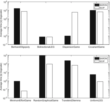
For the experiments on NF games in the LMFM case, we also consider eight GAMUT classes of structured normal-form games,BertrandOligopoly, Bidirectional-LEGs,MinimumEffortGames,RandomGraphicalGames,DispersionGames, Covari-antGames, TravelersDilemma and UniformLEGs, generating 10 instances with 2 followers andm=8 actions per player for each of them.
Throughout the section, the results of our experiments are compared w.r.t. com-puting time (in seconds) and (multiplicative) optimality gap.3 For both values, we report the arithmetic average for each game class and value ofmandn over the 10 corresponding instances. In all the boxplots that we report, the red dash indicates the median, the box extends from the 25th to the 75th percentile, and dotted lines denote the whole sample distribution. Outliers are highlighted with a red mark.
We adopt five solvers: BARON and SCIP (for globally optimal solutions to every formulation, apart from O-PM-LPFM-III which is an MILP), CPLEX (for globally optimal solutions to O-PM-LPFM-III, as well as to the oracle formulation for PM games in the implicit-enumeration and black-box methods), SNOPT (for locally opti-mal solutions to the formulations with purely continuous variables) and RBFOpt as the backbone of our black-box heuristic for pessimistic cases of LFNE. (We will, nevertheless, also experiment with it for some optimistic variants.) The O-NF-LPFM-implicit-enumeration algorithm is implemented in C. The experiments are run on a UNIX computer with a dual quad-core CPU at 2.33 GHz, equipped with 8 GB of RAM. Each algorithm is run using a single thread within a time limit of 3600 seconds. For the exact methods, we halt the execution whenever the optimality gap reaches 10−12%.4
9.1 O-NF-LMFM-I, II, and III (n=3)
We compare the different NF formulations when solved with BARON and SCIP. For
RandomGames instances, the average computing time and optimality gap for each combination of formulation and solver is reported in Fig.1as a function ofm.
The results obtained with the two solvers are quite different. BARON better per-forms on O-NF-LMFM-I (the formulation with purely continuous variables), while SCIP better performs on O-NF-LMFM-III (the “reformulated” formulation which con-tains binary variables introduced to remove nonquadratic terms from O-NF-LMFM-II,
3 The optimality gap is defined as minUB−LB LB 100,105
%, where LB and UB are, resp., the largest lower bound (corresponding to the best feasible solution) and the smallest upper bound found by the solver within the time limit. The min operator prevents an unbounded value for LB = 0. An optimality gap of 105 highlights that the method fails to produce a useful solution as, due to the payoffs being in[0,100],any
strategy of the leader can achieve, at least, a utility of 0.
4 Preliminary experiments with four tolerance values, namely 10−12%, 10−9%, 10−6% and 10−3%,
showed, for a larger tolerance, a negligible reduction in computing time by, at most and only in few instances, 2.5% with SCIP and 7.0% with BARON. The stricter tolerance was thus preferred.
n. of actions 0 5 10 15 20 25 Average time [s] 10-1 100 101 102 103 104 NF-LMFM-I NF-LMFM-II NF-LMFM-III
(a) Average times (BARON )
n. of actions
0 5 10 15 20 25
Average optimality gaps [%]
10-10 10-5 100 105 NF-LMFM-I NF-LMFM-II NF-LMFM-III
(b) Average gaps (BARON)
n. of actions 0 5 10 15 20 25 Average time [s] 10-2 100 102 104 NF-LMFM-I NF-LMFM-II NF-LMFM-III
(c) Average times (SCIP)
0 5 10 15 20 25 10−2 100 102 104 106
Average optimality gaps [%]
n. of actions
NF−LMFM−I NF−LMFM−II NF−LMFM−III
(d) Average gaps (SCIP)
Fig. 1 Computing times and optimality gaps obtained with the NF-LMFM formulations
as well as extra valid constraints). These results suggest that the formulation which is solved more efficiently with each solver is NF-LMFM-I with BARON and O-NF-LMFM-III with SCIP. These results are in line with the general computational behavior of BARON and SCIP, as the former tends to exhibiting a better performance on highly nonlinear and mostly continuous problems, whereas the latter becomes more efficient as the number of integer/binary variables of the problem increases.
Further inspecting Fig. 1, we notice that, with SCIP, O-NF-LMFM-III always outperforms O-NF-LMFM-II. This shows that SCIP is incapable of automatically constructing the reformulation obtained with O-NF-LMFM-III.
As to the computing times, the largestm for which at least a game is solved to optimality by BARON within the time limit ism=8 for O-NF-LMFM-I andm=7 for the other formulations. With SCIP, we reachm =9 with O-NF-LMFM-III and
m=3 with the other ones. In particular, SCIP with O-NF-LMFM-III always requires a shorter computing time than BARON with O-NF-LMFM-I for every number of actions.
In terms of optimality gaps, SCIP remarkably outperforms BARON. As one can see in Fig.1b, d, the gap achieved by BARON with O-NF-LMFM-I reaches 105%
BertrandOligopoly BidirectionalLEG DispersionGame CovariantGame
Average time [s] (logscale)
10-1 100 101 102 103 104 BARON SCIP
MinimumEffortGame RandomGraphicalGame TravelersDilemma UniformLEG
Average time [s] (logscale)
10-2 10-1 100 101 102 103 BARON SCIP
Fig. 2 Computing times obtained when solving formulation O-NF-LMFM-I with BARON and formulation O-NF-LMFM-III with SCIP for different GAMUT classes of structured games
when m ≥ 20. This is due to the solver returning an LB of 0 due to failing find a feasible solution in the time limit. Differently, the gap achieved by SCIP with O-NF-LMFM-III is below 15% for m up to m = 25. Such results suggest that, for games of this size, one can always achieve an almost constant gap, contrarily to what the intrinsic difficulty of the problem would suggest, namely an exponential quality degradation as the number of actions grows. Moreover, these results show that SCIP with O-NF-LMFM-III always finds a feasible solution (an NE) for the followers’ game and for some leader’s strategy, differently from the other pairs of solver and formulation.
These observations are substantially confirmed when experimenting with the same solver/formulation pair on the eight structured classes of NF games. The average computing times reported in Fig.2are indeed in line with the trends we observed for
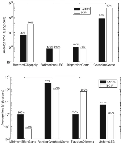
RandomGames, with SCIP outperforming BARON most of the times (on average). This trend becomes different when consideringDispersionGames, where SCIP per-forms less efficiently than for the other classes of games, achieving computing times which are considerably larger than those obtained with BARON. This is due to the solver failing to solve two game instances within the time limit. This can be better observed in Figure3which reports the computing times only for the instances that are solved to optimality with the two solvers, as well as the percentage of such instances. In particular, we observe that SCIP solves 91.875% of the instances on average, whereas BARON only solves 81.25%.
Fig. 3 Computing times only considering games for which the computations terminated; the percentage of instances solved to optimality is reported on top of each bar
9.2 O-PM-LMFM-I, II and III (n=3)
In Fig. 4, we report the computing times and the optimality gaps obtained with SCIP for games of the GAMUT classPolymatrixGames. Since the results obtained with BARON are similar to those we illustrated for NF games, we omit them for the sake of brevity.
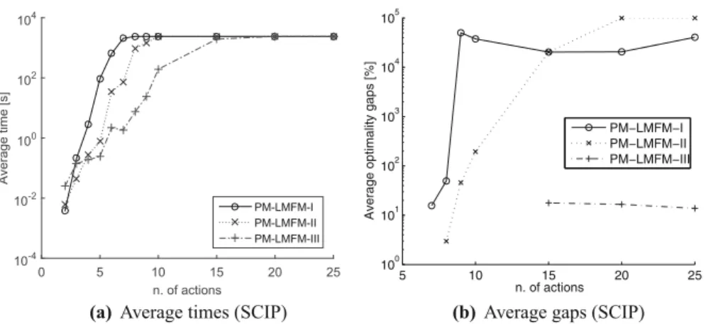
Within the time limit, the largest m for which at least an instance is solved to optimality ism=15. Form≤10, all instances are solved to within a gap of 0 (within the numerical tolerance we set). In particular, the optimality gap is always below 15% for instances with up tom=25, showing a trend which is substantially less steep than that for NF games. This suggests that PM games are, as expected, easier to solve. 9.3 O-NF-LMFM-I, local optimization (n=3)
In Fig.5, we report the experimental results obtained with SNOPT forRandomGames
n. of actions 0 5 10 15 20 25 Average time [s] 10-4 10-2 100 102 104 PM-LMFM-I PM-LMFM-II PM-LMFM-III
(a)Average times (SCIP)
5 10 15 20 25 100 101 102 103 104 105
Average optimality gaps [%]
n. of actions
PM−LMFM−I PM−LMFM−II PM−LMFM−III
(b) Average gaps (SCIP) Fig. 4 Computing times and optimality gaps with SCIP with O-PM-LMFM formulations
10−3 10−2 10−1 100 101 102 103 104 5 10 15 20 25 30 35 40 45 50 n. of actions Time [s]
(a) Average times (SNOPT)
0 10 20 30 40 50 60 70 80 3 4 5 6 7 n. of actions Gap [%]
(b) Average gaps (SNOPT) Fig. 5 Computing times and LBOPTratios obtained with SNOPT with O-NF-LMFM-I within 30 random restarts
for nonconvex problems, to obtain statistically more relevant results we run 30 restarts with different initial starting solutions, sampled uniformly at random from the sim-plices of the strategies of the three agents, and return the best solution found.
Figure5a shows that the computing times with SNOPT (cumulated over the 30 random restarts) are much shorter than the computing times required by BARON and SCIP, allowing for solving (to a local optimum) almost all the instances withm=20 within the time limit. Differently, as shown in Fig.5b the quality of the solutions returned by SNOPT (measured as their ratio over the value of an optimal solution found by SCIP or BARON) is rather poor even with very few actions. Indeed, the median of the ratios is between 10 and 20% for games with up tom =7. This emphasizes the effectiveness of our approach based on spatial-branch-and-bound methods.
9.4 O-NF/PM-LMFM-III (n≥4)
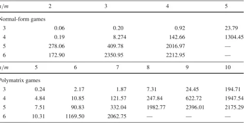
In Table1, we report the average computing times obtained with SCIP when employ-ing formulations O-NF-LMFM-III and O-PM-LMFM-III for games with 4 players
Table 1 Computing times (in seconds) with SCIP and O-NF/PM-LMFM-III, within a time limit of 3600 s n/m 2 3 4 5 Normal-form games 3 0.06 0.20 0.92 23.79 4 0.19 8.274 142.66 1304.45 5 278.06 409.78 2016.97 — 6 172.90 2350.95 2212.95 — n/m 5 6 7 8 9 10 Polymatrix games 3 0.24 2.17 1.87 7.31 24.45 194.71 4 4.84 10.85 121.57 247.84 622.72 1947.54 5 7.51 90.83 332.04 1982.77 2396.01 2175.29 6 10.31 1169.50 2062.75 — — —
or more. In the time limit, we can solve NF games with up to m = 5 for n ≤ 4 (corresponding to up tomn = 625 different outcomes and nmn = 2500 different payoffs) and up tom =4 forn ≤6 (corresponding to up tomn =4096 outcomes andnmn = 24,576 payoffs). Quite interestingly, with our methods we can tackle instances of a size comparable to that of the largest instances used in Porter et al. (2008) (such instances are generated with GAMUT (Nudelman et al.2004) and are comparable to the ones in our test bed) to evaluate a set of algorithms proposed to find an NE (in a single-level problem), in spite of our problem being clearly harder (as it admits the former as a subproblem). With PM games, our algorithms scale much better, allowing for finding exact solutions to PM games with up tom=10 forn≤5 and up tom=7 forn ≤6.
9.5 O/P-NF/PM-LMFM-blackBox
When experimenting with the black-box method, we first consider the optimistic case for NF games as, for it, we can compare the quality of the solutions we find to either the optimal solution value or its tightest upper bound. Namely, we compare O-NF-LMFM-blackBox to O-NF-LMFM-III, the latter solved with SCIP within the time limit. The results are reported in Fig.6.
In Fig. 6a, we observe, on average and form ≤ 10, that the black-box method yields solutions to within 90% of the optimal ones found with SCIP. This suggests that the method might be sufficiently accurate. As shown in Fig.6b, form≥ 10 the burden of calling SCIP to solve the oracle formulation becomes too large, making the black-box algorithm impractical.
An interesting result, see Fig.6a, concerns the gap between the utility of the leader at an optimistic LFNE or at a pessimistic LFNE. On the instances solved to optimality (m≤5), where we can verify the quality of the heuristic solutions, we see that the gap is rather small, suggesting that, inRandomGamesinstances generated with GAMUT,
2 5 10 15 50 60 70 80 90 100 Average value n. of actions O−NF−LMFM−III (SCIP) O−NF−LMFM−BlackBox P−NF−LMFM−BlackBox
(a) Average objective
2 5 10 15 0 20 40 60 80 100 120 140 160
Average evaluation time
n. of actions O−NF−LMFM−BlackBox P−NF−LMFM−BlackBox
(b) Average oracle time Fig. 6 Performance of the black-box approach for O/P-NF-LMFM compared to O-NF-LMFM-III
2 5 10 15 60 80 100 120 140 160 180 Average value n. of actions O−PM−LMFM−III (SCIP) O−PM−LMFM−BlackBox P−PM−LMFM−BlackBox
(a) Average objective
2 5 10 15 0 0.1 0.2 0.3 0.4 0.5 0.6 0.7 0.8
Average evaluation time
n. of actions
O−PM−LMFM−BlackBox P−PM−LMFM−BlackBox
(b) Average oracle time Fig. 7 Performance of the black-box approach for O/P-PM-LMFM compared to O-PM-LMFM-III
the leader can manage to force the followers to play a strategy which provides the leader with a utility not dramatically smaller than that which they would obtain in an optimistic LFNE.
In Fig.7, we report analogous results obtained with polymatrix games. In the time limit, we compare O-PM-LMFM-III solved with SCIP to O-PM-LMFM-blackBox. Differently from the NF case, Fig.7b shows that, for PM games, the computing time needed to solve the oracle formulation (which is an MILP in this case) is much smaller and scales much better withm. Except for the case ofm = 2, Fig.7a allows us to draw comparable conclusions to those that we have drawn for the NF case, with the leader achieving, in the pessimistic case, solutions that are not too far away from the corresponding optimistic ones w.r.t. their utility.
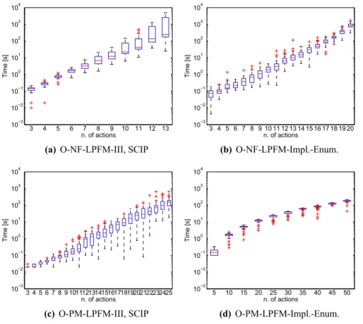
9.6 O-NF/PM-LPFM and O-NF/PM-implicit-enumeration (n=3)
Lastly, we focus on the case where the leader is restricted to pure strategies. We report the results in terms of computing times obtained by imposingδ ∈ {0,1}m in
10−3 10−2 10−1 100 101 102 103 104 3 4 5 6 7 8 9 10 11 12 13 n. of actions Time [s]
(a) O-NF-LPFM-III, SCIP
10−3 10−2 10−1 100 101 102 103 104 3 4 5 6 7 8 9 10 11 12 13 14 15 16 17 18 19 20 n. of actions Time [s] (b) O-NF-LPFM-Impl.-Enum. 10−3 10−2 10−1 100 101 102 103 104 3 4 5 6 7 8 9 10111213141516171819202122232425 n. of actions Time [s] (c) O-PM-LPFM-III, SCIP 10−3 10−2 10−1 100 101 102 103 104 5 10 15 20 25 30 35 40 45 50 n. of actions Time [s] (d) O-PM-LPFM-Impl.-Enum. Fig. 8 Computing times on NF/PM-LPFM instances with O-NF/PM-LPFM-III (a/c) and O-NF/PM-LPFM-implicit-enumeration (b/d), using SCIP/CPLEX
O-NF/PM-LPFM-III with SCIP forRandomGamesin Fig.8a, b and with CPLEX for
PolymatrixGames(for which the formulation becomes an MILP) in Fig.8c, d. Interest-ingly, by imposing a binaryδto tackle the LPFM case the size of the largest instances solvable within the time limit increases fromm=9 tom=13 inRandomGamesand fromm=15 tom=25 forPolymatrixGameswhen compared to the LMFM case.
For bothRandomGamesandPolymatrixGames, a dramatic performance improve-ment is obtained with O-NF/PM-LPFM-implicit-enumeration: with it, the size of the largest instance that we can solve increases fromm=13 tom=20 forRandomGames
and fromm=25 tom=50 forPolymatrixGames. As expected, the computing times forPolymatrixGamesare much smaller (due to only requiring the solution of an MILP at each step), allowing us to solve to optimality much larger instances.
10 Conclusions and future work
We have studied game-theoretic leader-follower (Stackelberg) situations with a bilevel structure where multiple followers play a Nash equilibrium once the leader has