Bayesian nonlinear regression for large p small n problems

(1)

Contents lists available atSciVerse ScienceDirect

Journal of Multivariate Analysis

journal homepage:www.elsevier.com/locate/jmva

Bayesian nonlinear regression for large

p

small

n

problems

Sounak Chakraborty

a

, Malay Ghosh

b

, Bani K. Mallick

c,∗

a_{Department of Statistics, University of Missouri-Columbia, 209F Middlebush Hall, Columbia, MO 65211, USA} b_{Department of Statistics, University of Florida, 103 Griffin/Floyd Hall, Gainesville, FL 32611-8545, USA} c_{Department of Statistics, Texas A & M University, 415D Blocker Building, College Station, TX 77843-3143, USA}

a r t i c l e i n f o Article history:

Received 8 February 2010 Available online 6 February 2012 AMS subject classifications: 62J02 62M20 62H99 62G08 62F15 Keywords:

Bayesian hierarchical model Empirical Bayes

Gibbs sampling Markov chain Monte Carlo Metropolis–Hastings algorithm Near infrared spectroscopy Relevance vector machine Reproducing kernel Hilbert space Support vector machine Vapnik’sϵ-insensitive loss

a b s t r a c t

Statistical modeling and inference problems with sample sizes substantially smaller than the number of available covariates are challenging. This is known as large psmalln problem. Furthermore, the problem is more complicated when we have multiple correlated responses. We develop multivariate nonlinear regression models in this setup for accurate prediction. In this paper, we introduce a full Bayesian support vector regression model with Vapnik’s ϵ-insensitive loss function, based on reproducing kernel Hilbert spaces (RKHS) under the multivariate correlated response setup. This provides a full probabilistic description of support vector machine (SVM) rather than an algorithm for fitting purposes. We have also introduced a multivariate version of the relevance vector machine (RVM). Instead of the original treatment of the RVM relying on the use of type II maximum likelihood estimates of the hyper-parameters, we put a prior on the hyper-parameters and use Markov chain Monte Carlo technique for computation. We have also proposed an empirical Bayes method for our RVM and SVM. Our methods are illustrated with a prediction problem in the near-infrared (NIR) spectroscopy. A simulation study is also undertaken to check the prediction accuracy of our models.

1. Introduction

Regression techniques are amongst some of the most widely used methods in applied statistics. Given a response variable

Y, and a set of covariatesX

=

(

X1

,

X2

, . . . ,

Xp

)

T, one is often interested in predicting further responses for new values of the

covariates. The problem becomes complicated when the sample sizenis substantially smaller than the number of covariates

p. This is known as the largepsmallnproblem or high dimension low sample size problem. The usual way to handle the problem is to reduce the number of covariates by using variable selection [5] or projecting them to lower dimension using principal component or other related methods [27].

Most of the existing methods for variable selection or projections are based on linear relationship between the response and the covariates which may not be very realistic. Recent advances in computer power have allowed statisticians to consider richer classes of nonlinear regression models. Due to the largepsmallnproblem, these methods are usually inapplicable in these situations. We use instead the reproducing kernel Hilbert space (RKHS) methodology for these problems. We are particularly interested in the analysis of multivariate data with correlated responses.

∗_{Corresponding author.}

(2)

One important motivating application arises from the near infrared (NIR) spectroscopy. An experiment involving spectral measurements typically produces more covariates (wavelengths/channels) than calibration measurements (samples). Traditional stepwise regression methods fail miserably in these circumstances because of the lack of necessary samples. Chemometricians often use principal component regression (PCR), partial least squares (PLS) regression, multiple linear regression, and ridge regression to overcome these limitations. Both principal component regression and partial least squares regression, produce factor scores as linear combinations of the original predictor variables, so that there is no correlation between the factor score variables used in the predictive regression model. But they differ in the methods used in extracting the factor scores. In short, PCR produces the weight matrix reflecting the covariance structure between the predictor variables, while PLS regression produces the weight matrix reflecting the covariance structure between the predictor and response variables. We know from chemistry and optics that reflectance or absorbencies are linearly related to the concentrations, (Beer–Lambert Law). There is deviation from this law for reasons such as optical scattering, autofluorescence etc. The resultant nonlinearities impair the accuracy of prediction based on linear relationships. The problem becomes more complicated when there are multiple constituents under investigation as we then need to develop multivariate nonlinear regression models for prediction.

One of the models which we will consider for this purpose is support vector machine (SVM). The classical support vector machine (SVM) algorithm, despite its success in regression and classification, suffers from a serious disadvantage: it cannot provide any probabilistic outputs. Law and Kwok [12] introduced a Bayesian formulation of SVM for regression, but they did not carry out a full Bayesian analysis and used instead certain approximations for the posterior. A similar remark applies to Sollich [20] who considered SVM in the classification context. More recently, Mallick et al. [14] considered a Markov chain Monte Carlo (MCMC) based full Bayesian analysis for classification where the number of covariates was far greater than the sample size. However, it was designed only for binary classification, and cannot be used for continuous regression problems with multivariate responses.

As an alternative to SVM, Tipping [21,22] and Bishop and Tipping [4] introduced relevance vector machines (RVM’s). RVM’s are suitable for both regression and classification, and are amenable to probabilistic interpretation. However, these authors did not perform a full Bayesian analysis. They obtained type II maximum likelihood [9] estimates of the prior parameters, which do not provide predictive distribution of the future observations. Also, their procedure cannot provide measures of precision associated with the estimates. However, none of the above mentioned methods can handle multivariate correlated responses.

The present article addresses a full Bayesian analysis of regression problems whenp, the number of covariates far outnumbern, the sample size and the response is multivariate. The SVM approach is based on reproducing kernel Hilbert spaces (RKHS) and a multivariate extension of Vapnik’s [23]

ϵ

-insensitive loss function. We also consider the multivariate extension of RVM-based analysis in this context, once again by using RKHS. Ours is a full hierarchical Bayesian model. Instead of relying on the type II maximum likelihood estimates of the prior parameters, we assign distributions to these parameters. In this way, we can capture the uncertainty in estimating these parameters, and consequently get more reliable measures of precision associated with the Bayes estimates. A key feature of our method is to treat the kernel parameter in the model as unknown and infer about it with all other parameters. We obtain a more accurate prediction by the mixing of several RVM (or SVM) models through the kernel parameter. Due to analytical intractability of posteriors, we use the MCMC numerical integration technique for implementation of the Bayes procedure.

Both methods are illustrated with a real data set, discussed in [6]. The available measurements are the near infrared reflectance spectrum of biscuit dough pieces at 700 equally spaced wavelengths. The aim is to predict the composition i.e., the fat, sugar, flour, and water content of the dough pieces using the spectral variables. We compare our procedure with some of the classical methods like stepwise multiple linear regression (MLR), PLS, PCR, and classical support vector regression as well as Bayesian wavelet regression [6] based on mean square errors of prediction (MSEP). It turns out that, our multivariate Bayesian RVM and SVM performs better than all competing methods, for all the components except fat, where stepwise MLR has the best performance.

Apart from introducing hierarchical Bayes multivariate RVM and SVM models, we have also suggested an empirical Bayes analysis for our RVM and SVM models in the multivariate set up. In our empirical Bayes approaches we estimate the kernel parameter from the data by maximizing the marginal posterior. The empirical Bayes results are tabulated inTables 1–3.

Section2of this paper introduces the RKHS-based regression method and some related results. The multivariate Bayesian RVM and SVM are introduced in Sections3and4. Section5discusses prediction of a future observation. Section6contains the biscuit dough example. In Section7, we provide a simulation study. In Section8we introduce empirical Bayes SVM and RVM. Finally, some concluding remarks are made in Section9.

2. Regression method based on RKHS

For a regression problem, we have a training set

{

yi,xi

}

,

i

=

1

, . . . ,

n, whereyiis the response variable andxiis the vector

of covariate of sizepcorresponding toyi. Given the training data our goal is to find an appropriate functionf

(

x

)

to predict

the responsesyin the test set based on the covariatesx. This can be viewed as a regularization problem of the form

min f∈H



_n



i=1 L

(

yi

,

f

(

xi

))

+

λ

J

(

f

)



(1)

(3)

Table 1

Mean squared errors of prediction on the 39 biscuit dough pieces in the validation set. The number in parenthesis is the standard deviation of MSEP.

Method Fat Sugar Flour Water

Stepwise MLR 0.044 1.188 0.722 0.221 Decision theory 0.076 0.566 0.265 0.176 PLS 0.155 0.578 0.369 0.107 PCR 0.156 0.605 0.378 0.103 BWR 0.063 0.449 0.348 0.050 CSVM-P 0.067 0.609 0.362 0.105 CSVM-G 0.097 0.715 0.395 0.101

Hyperparameter choice (i)

MBRVM 0.057 (0.003) 0.314 (0.018) 0.252 (0.019) 0.031 (0.005) MBSVM 0.062 (0.003) 0.339 (0.019) 0.229 (0.019) 0.045 (0.006) Hyperparameter choice (ii)

MBRVM 0.057 (0.004) 0.320 (0.017) 0.236 (0.018) 0.038 (0.004) MBSVM 0.065 (0.003) 0.343 (0.019) 0.232 (0.018) 0.050 (0.006) EMBRVM 0.065 (0.004) 0.439 (0.019) 0.309 (0.020) 0.075 (0.006) EMBSVM 0.074 (0.004) 0.477 (0.020) 0.341(0.018) 0.056 (0.006)

Table 2

Mean squared errors of prediction on the 39 biscuit dough pieces in the validation set when the sample 23 is included in the training set. The number in parenthesis is the standard deviation of MSEP.

Hyperparameter choice (i)

MBRVM 0.097 (0.008) 3.111 (0.150) 2.689 (0.131) 0.122 (0.009) MBSVM 0.081 (0.005) 0.613 (0.021) 0.412 (0.020) 0.132 (0.005) EMBRVM 0.161 (0.007) 5.325 (0.144) 3.982 (0.149) 0.176 (0.007) EMBSVM 0.097 (0.006) 0.742 (0.025) 0.369 (0.023) 0.153 (0.007)

Table 3

Average mean squared errors of prediction in the simulated data set. The number in parenthesis is the standard deviation of MSEP.

Stepwise MLR 0.107 (0.015) 2.512 (0.231) 1.802 (0.276) 0.953 (0.039) Decision theory 0.231 (0.013) 0.809 (0.199) 0.665 (0.162) 0.703 (0.042) PLS 0.295 (0.011) 0.997 (0.064) 0.856 (0.071) 0.715 (0.053) PCR 0.310 (0.014) 0.971 (0.061) 0.890 (0.069) 0.801 (0.055) BWR 0.096 (0.016) 0.698 (0.026) 0.481 (0.029) 0.407 (0.105) CSVM-P 0.617 (0.027) 1.304 (0.201) 0.913 (0.174) 0.835 (0.113) CSVM-G 0.705 (0.029) 1.518 (0.315) 1.195 (0.169) 0.879 (0.115) Hyperparameter choice (i)

MBRVM 0.076 (0.017) 0.480 (0.027) 0.279 (0.047) 0.178 (0.019) MBSVM 0.093 (0.019) 0.563 (0.030) 0.321 (0.041) 0.385 (0.031) EMBRVM 0.086 (0.021) 0.512 (0.025) 0.319 (0.053) 0.217 (0.031) EMBSVM 0.098 (0.017) 0.663 (0.037) 0.473 (0.061) 0.488 (0.040)

whereL

(

y

,

f

(

x

))

is a loss function,J

(

f

)

is a penalty functional,

λ >

0 is the smoothing parameter, andH is a space of functions on whichJ

(

f

)

is defined. In this article, we considerH to be a reproducing kernel Hilbert space (RKHS) with kernelK, and we denote it byHK. A formal definition of RKHS in given in [2,19,24].

For anh

∈

HK, iff

(

x

)

=

β

0

+

h

(

x

)

, we takeJ

(

f

)

= ∥

h

∥

2HKand rewrite(1)as

min f∈HK



_n



i=1 L

(

yi

,

f

(

xi

))

+

λ

∥

h

∥

2HK



(2)

(4)

The estimate ofhis obtained as a solution of(2). It can be shown that the solution is finite-dimensional [24] and leads to a representation off [11,26] as f_λ

(

x

)

=

β

₀

+

n



i=1

β

iK

(

x

,

xi

).

(3)

It is also a property of RKHS that

∥

h

∥

2_H K

=

n



i,j=1

β

i

β

jK

(

xi

,

xj

).

(4)

Representation offin above form is of special interest to us, because cases when the number of covariatespis much larger than the number of data points, we effectively reduce the dimension of covariates frompton. To obtain the estimate off_λ

we substitute(3)and(4)in(2)and then minimize it with respect to

β

=

(β

₀

, . . . , β

_n

)

and the smoothing parameter

λ

. The other parameters inside the kernelKmay be chosen by generalized approximate cross validation.

Similarly, for multivariate regression whenf

(

x

)

=

(

f1

(

x

), . . . ,

fq

(

x

))

is aq-tuple function we can have similar results

based on RKHS as the univariate case. Here we considerf

(

x

)

∈



q

j=1

(

{

1

} +

HKj

)

, the product space ofqreproducing kernel

Hilbert spacesHKjforj

=

1

, . . . ,

q. In other words, each component can be expressed as

β

0j

+

hj

(

x

)

withhj

∈

HKj. Unless

there is compelling reason to believe thatHKjshould be different forj

=

1

, . . . ,

q, we will assume that they are the same

RKHS denoted byHK. All results stated before also hold in this framework.

Regarding the lossL

(

y

,

f

(

x

))

as the negative of the log-likelihood, our problem is equivalent to maximization of the penalized log-likelihood

−

n



i=1 L

(

yi

,

f

(

xi

))

−

λ

∥

h

∥

2Hk

.

(5)

This duality between ‘‘loss’’ and ‘‘likelihood’’, particularly viewing the loss as the negative of the log-likelihood, is referred in the Bayesian literature as the ‘‘logarithmic scoring rule’’ [3, p. 688].

3. Hierarchical Bayes RVM for multivariate regression

The support vector machine (SVM) is a highly sophisticated technique for regression and classification. It is well known that SVM can be derived as the minimizer of the function



n

i=1L

(

yi

,

f

(

xi

))

+

λ

∥

h

∥

2HK in RKHS [25]. Despite its widespread

success, the classical SVM suffers from some important limitations, notably the absence of probabilistic output i.e. it makes point predictions rather than generating predictive distributions. Recently Tipping [21] has formulated the relevance vector machine (RVM), a probabilistic model whose functional form is equivalent to the SVM with a least square loss function (also known as LS-SVM). Law and Kwok [12] considered a Bayesian SVM model with Vapnik’s

ϵ

-insensitive robust loss function, a detailed discussion is provided in the next section. The original treatment of RVM relied on the use of type II maximum likelihood [9] estimates of the hyper-parameters. In this paper we formulate both SVM and RVM in a complete hierarchical Bayesian paradigm based on the RKHS formulation, as discussed in the previous section.

If we assume thatfis generated from RKHS with the kernel functionK

(., .)

, using the representation theorem(3)we can expressf as f

(

xi

)

=

β

0

+

n



j=1

β

jK

(

xi

,

xj

|

θ)

(6)

whereKis a positive definite function of the covariatesxinvolving some unknown parameter

θ

. Hence,

yi

=

f

(

xi

)

+

η

i

=

KiT

β

+

η

i (7)

where

η

i

i.i.d.

∼

N

(

0

, σ

2

),

β

=

(β

₀

, . . . , β

_n

)

T, andKi

=

(

1

,

K

(

xi

,

x1

|

θ), . . . ,

K

(

xi

,

xn

|

θ))

T

,

i

=

1

, . . . ,

n. However, when the

responses are multivariate or a vector of measurements modeling each element of the response vector separately using(7)

rules out any correlation among them.

Under the multivariate response set up let us define the data setD

=

((

y1

,

x1

), . . . , (

yn

,

xn

))

, consisting of multivariate

responsesyi

=

(

yi1

, . . . ,

yiq

)

T (withqcomponents) and explanatory variablesxi

=

(

xi1

, . . . ,

xip

)

T

,

i

=

1

, . . . ,

n. We

introducenlatent variablesz1

, . . . ,

zn, wherezi

=

(

zi1

, . . . ,

ziq

)

Tand assume that conditional onzi

,

yi’s are independent.

Also conditional onz_ithe all components ofy_iare independent among themselves. Thus we can write

yi

=

zi

+

η

i (8)

where

η

_i

=

(η

_i₁

, . . . , η

_iq

)

T_{is a multivariate normal random variate with mean zero and variance}_V

=

_diag

(σ

2

1

, . . . , σ

q2

)

.

(5)

variance. In this way we allow any possible heteroscedasticity in the components ofy_i. This gives enormous flexibility in the modeling. In the regular cases we put a variance covariance matrix on the variance of

η

_i and assign a inverse Wishart prior on it. But it largely restrains the modeling, as by putting an inverse Wishart distribution we are effectively giving same degrees of freedom for all the variance components. Also, we establish the dependence between different components of the response vectoryiby introducing the latent variablesziand connectziwithf

(

xi

)

=

(

f1

(

xi

), . . . ,

fq

(

xi

))

T

byzi

=

f

(

xi

)

+

δ

i

,

δ

i

=

(δ

i1

, . . . , δ

iq

)

Tbeing the vector of the residual random effects. Assuming thatf is generated from

the product space ofqRKHS’sHKwith the kernel functionK

(., .)

, the representation theorem of Kimeldorf and Wahba(3)

leads to the representation

zi

=

Ki0

β

+

δ

i (9)

whereK_i0

=

Iq



K_iT

,

β

=

(β

T₁

, . . . ,

β

T_q

)

T

,

β

_j

=

(β

₀_j

, . . . , β

_nj

)

T, and

δ

i

i.i.d.

∼

Nq

(

0

,

6

)

. The

δ

iintroduce dependence in the

components ofz_i, which in turn creates association among the components ofy_i. In the above model(9)the unknown parameters are

β,

3

=

diag

(

31

, . . . ,

3q

),

V

,

6, and

θ

. Conditional on these parameters our latent variablezifollow

zi

|

β,

6

, θ

ind

∼

Nq

(

Ki0

β,

6

),

(10)

wherei

=

1

, . . . ,

n. We assign hierarchical priors to the unknown parameters

β,

3

,

V

,

6, as follows

β

j

|

3j ind

∼

Nn+1

(

0

,

3 −1 j

)

;

3j

=

diag

(λ

0j

, . . . , λ

nj

)

(11) 6

∼

IW

(ψ,

Q

)

(12)

σ

2 j i.i.d.

∼

IG

(γ

1

, γ

2

)

(13)

λ

ij i.i.d.

∼

Gamma

(

c

,

d

)

(14) wherej

=

1

, . . . ,

q

.

In the above prior formulation

λ

0j-s are fixed at a small value to induce a flat prior on the intercept term

β

0j, but

other

λ

ij-s are kept unknown. A Gamma

(α, ξ)

distribution for a random variableUhas density function proportional to

exp

(

−

ξ

u

)

uα−1, while the reciprocal ofUwill then said to have a inverse gamma distribution is denoted by IG

(α, ξ)

. An inverse Wishart distribution with parameters

ψ

andQ for a random variableShas distribution function proportional to

f

(

S

)

∝ |

S

|

−12(ψ+p+1)_exp



−

1

2tr

(

S −1_Q

)



. We refer to it as IW

(ψ,

Q

)

.

The matrix with

(

i

,

j

)

th elementKij

=

K

(

xi

,

xj

|

θ)

is known as the kernel matrix. The usual choices are (i) the Gaussian

kernelK

(

xi

,

xj

|

θ)

=

exp

{−

∥xi−xj∥2

2θ

}

and (ii) the polynomial kernel,K

(

xi

,

xj

|

θ)

=

(

x T

ixj

+

1

)

θ. The

θ

parameter associated

with the kernel functionK

(., .

|

θ)

controls the shape of the kernel. The choice of the prior distribution for

θ

depends on the adopted kernel functionK

(., .

|

θ)

. In this paper we use the polynomial kernel, where

θ

is the degree of the polynomial. Therefore here we assign a discrete uniform prior on

θ

as follow

θ

∼

U

{

1

, . . . ,

C

}

.

(15)

The joint posterior is thus given by

π(β,

3

,

z

,

V

,

6

, θ

|

y

)

∝

exp



−

1 2 n



i=1

(

yi

−

zi

)

TV−1

(

yi

−

zi

)



1

|

6

|

n/2exp



−

1 2 n



i=1

(

zi

−

Ki0

β)

T6 −1

(

_z i

−

Ki0

β)



× |

6

|

−12(ψ+q+1)_exp



−

1 2tr

(

6 −1_Q

)



1

|

3

|

−1/2exp



−

1 2

β

′ 3

β



×

q



j=1 exp



−

γ

2

σ

2 j



(σ

2 j

)

−γ1−1

×

n



i=1 q



j=1 exp

(

−

d

λ

ij

)λ

cji−1

.

(16)

3.1. Conditional distributions and posterior sampling of the parameters

The posterior distribution described in(16)is complex, and implementation of the Bayesian procedure requires MCMC sampling techniques, and in particular, the Gibbs sampling [8] and Metropolis–Hastings (MH) algorithm [16,7]. The Gibbs sampler generates posterior samples using the conditional densities of the model parameters. We list the conditional posterior distributions as follows:

(i)

β

|

3

,

z

,

V

,

6

, θ,

y

∼

Nq(n+1)

(µ

∗β

,

Vβ∗

)

,

where

µ

∗_β

=

V_β∗



_in₌₁K_i0T6−1zi



(6)

(ii) 6

|

β,

3

,

z

,

V

, θ,

y

∼

IW

(ψ

∗

,

Q∗

)

, where

ψ

∗

=

n

+

ψ,

Q∗

=

_Q

+



n i=1

(

zi

−

Ki0

β)(

zi

−

Ki0

β)

T. (iii)

σ

_j2

|

β,

3

,

z

,

6

, θ,

yind

∼

IG

(γ

₁∗

, γ

₂∗

),

j

=

1

, . . . ,

q, where

γ

∗ 1

=

n

/

2

+

γ

1

, γ

2∗

=



n i=1 (yij−zij)2 2

+

γ

2. (iv)

λ

ij

|

β,

V

,

z

,

6

, θ,

y ind

∼

Gamma

(

c∗

,

_d∗

),

_j

=

₁

, . . . ,

_q

;

_i

=

₁

, . . . ,

_n_, wherec∗

=

_c

+

₁

/

_{2 and}_d∗

=

βij2 2

+

d. (v) zi

|

3

,

β,

V

,

6

, θ,

y ind

∼

Nq

(µ

∗zi

,

6 ∗ zi

)

, where

µ

∗ zi

=

6 ∗ zi

(

V −1_y i

+

6−1Ki0

β)

;6 ∗ zi

=



V−1

+

₆−1



−1 . (vi) p

(θ

|

3

,

β,

V

,

6

,

z

,

y

)

∝

exp



−

1₂



n i=1

(

zi

−

Ki0

β)

T6 −1

(

_z i

−

Ki0

β)



.

The conditional distributions given in (i)–(v) are standard and it is easy to generate samples from them. The conditional distribution in (vi) is not standard and we need to employ the MH algorithm. We use the above listed conditional distributions for constructing a Gibbs sampler through these following steps:

•

Step 1. Update

β

by sampling from the conditional distribution (i).

•

Step 2. Update6by sampling from the conditional distribution (ii).

•

Step 3. Update

σ

2

j

,

j

=

1

, . . . ,

q, by sampling from the conditional distribution (iii).

•

Step 4. Update

λ

ij

,

j

=

1

, . . . ,

q

,

i

=

1

, . . . ,

n, by sampling from the conditional distribution (iv).j

=

1

, . . . ,

q

;

i

=

1

, . . . ,

n

•

Step 5. Updatezi

,

i

=

1

, . . . ,

n, by sampling from the conditional distribution (v).

•

Step 6. Update ofK0_{is equivalent to the update of}

θ

_{and we need a Metropolis–Hastings algorithm to sample from the}

conditional distribution of

θ

given in (vi). If

θ

is the current value, draw a candidate value

θ

∗_{from the discrete}

uniform distribution U

{

1

, . . . ,

C

}

. Accept the

θ

∗as a new value of

θ

with acceptance probability

α

=

min



1

,

p

(θ

∗

|

₃

,

β,

V

,

6

,

z

,

y

)

p

(θ

|

3

,

β,

V

,

6

,

z

,

y

)



.

(17)

In the multivariate relevance vector machine discussed above, we effectively try to minimize the squared error loss function and use separate smoothing parameters

λ

ijfor different

β

ij. The smoothing parameters determine the tradeoff between

training accuracy and model complexity. The multiple smoothing parameter is also used by Tipping [21]. By having multiple smoothing parameters over a single one we are effectively control each of the regression coefficients separately, thereby introducing sparseness in the model. Moreover, the smoothing is controlled separately for each component of the response vector adding more flexibility in our model. The model discussed in this section will be referred to as the multivariate Bayesian relevance vector machine orMBRVM.

4. Hierarchical Bayes SVM for multivariate regression

In this section, we develop our multivariate SVM based on RKHS under complete Bayesian framework using a modified Vapnik’s

ϵ

-insensitive loss function for the multivariate response cases. Law and Kwok [12] proposed a Bayesian SVM, however their model was based on univariate framework and cannot handle correlated multivariate responses. Moreover, they did not carry out a full hierarchical Bayesian analysis and used instead type II maximum likelihood to estimate the prior parameters.

For regression problems with univariate response Vapnik [23] introduced the

ϵ

-insensitive loss function as follows

L

(

y

,

f

(

x

))

= |

y

−

f

(

x

)

|

_ϵ

=



0 if

|

y

−

f

(

x

)

| ≤

ϵ

|

y

−

f

(

x

)

| −

ϵ

otherwise

.

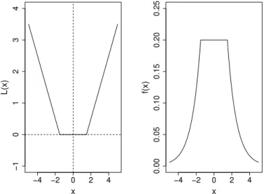
(18) This loss function (Fig. 1) ignores errors of size less than

ϵ

but penalizes in a linear fashion when the function deviates more than

ϵ

amount. This makes the fitting less sensitive to the outliers. It is interesting to note that like other loss functions or error measures in robust regression [10], Vapnik’s

ϵ

-insensitive loss function also has linear tails beyond

ϵ

. But in addition it flattens the contributions of those cases with small residuals.

To construct a hierarchical model for regression using the Vapnik’s univariate loss function(18)we can introducen

latent variableszi

i.i.d.

∼

N

(

f

(

x_i

), σ

2

),

_i

=

₁

, . . . ,

_n_{. Such that}_y

i’s are conditionally independent givenzi. Introduction of the

latent variables makes the calculations particularly simple. The likelihood ofyiconditional onzi, corresponding to Vapnik’s

univariate loss(18)as suggested by Law and Kwok [12], is given by

(7)

Fig. 1. The figure in the left hand side represents Vapnik’sϵ-insensitive (ϵ=1) loss function. The figure in the right hand side represents the corresponding likelihood.

Fig. 2. Ourϵ-insensitive loss function whenq=2 andρ1=ρ2=1(ϵ=1).

It can be shown that this pdf (Fig. 1) can be written as a mixture of a truncated Laplace distribution and a uniform distribution as follows p

(

yi

|

zi

)

=

ρ

2

(

1

+

ϵρ)

exp

{−

ρ

|

yi

−

zi

|

ϵ

}

=

ρ

2

(

1

+

ϵρ)

[I

(

|

yi

−

zi

|

> ϵ)

exp

{−

ρ(

|

yi

−

zi

| −

ϵ)

} +

I

(

|

yi

−

zi

| ≤

ϵ)

]

=

p1

(

Truncated Laplace

(

zi

, ρ))

+

p2

(

Uniform

(

zi

−

ϵ,

zi

+

ϵ))

wherep1

=

1

+

ϵρ

,

p2

=

ϵρ

1

+

ϵρ

.

(20)

A Laplace

(θ, ρ)

distribution for a random variableUhas pdf proportional to exp

(

−

ρ

|

u

−

θ

|

)

. When the response is multivariate we generalize Vapnik’s

ϵ

-insensitive loss to (Fig. 2)

L

(

yi

,

f

(

xi

))

= ∥

yi

−

f

(

xi

)

∥

ϵ

=

q



j=1

ρ

j

|

yij

−

fj

(

xi

)

|

ϵ

,

(21)

wheref

(

xi

)

=

(

f1

(

xi

), . . . ,

fq

(

xi

))

Tandyi

=

(

yi1

, . . . ,

yiq

)

T(withqcomponents). Similar to the univariate

ϵ

-insensitive loss (18)and(19), in the multivariate case for(21)we can introduce latent vectorszi

i.i.d.

∼

Nq

(

f

(

xi

), σ

2Iq

),

i

=

1

, . . . ,

n. The

(8)

p

(

y_i

|

z_i

)

∝

exp

{−∥

y_i

−

z_i

∥

_ϵ

}

.

(22) From(22)notice that, conditional onzieach component ofyivector follows the mixture distribution given in(20). As in

Section3(for MBRVM) here also we assume that the underlying functionfis generated from the product space ofqRKHS’s and use the representation theorem(3)to connect the latent variableszwithf. Therefore,zi

=

f

(

xi

)

+

δ

i, where

δ

iis the

vector of the residual random effects that account for any unexplained source of variation not included in the model. As the

f is generated from RKHS, following the representation(6)theziare modeled aszi

=

Ki0

β

+

δ

i.

We specify hierarchical priors on

β,

6

,

3, and

θ

as in(11),(12),(14)and(15). In addition to that we assign flat priors for the scale parameter

ρ

jas

ρ

j

i.i.d.

∼

U

(

rL

,

rU

)

j

=

1

, . . . ,

q

.

(23)

Asymptotically if the

ϵ

goes to infinity in(20), we get the uniform likelihood, but if it goes to 0 we get the usual Laplace likelihood when

ρ

is fixed. So instead of keeping

ϵ

fixed, as in a classical SVM we assigned prior to

ϵ

. However, we observed that the performance of SVM decayed rapidly for priors spreading outside the range

(

0

,

1

)

. More detailed justifications are provided in [12]. Hence we have considered

ϵ

∼

Beta

(

k1

,

k2

).

(24)

Our multivariate Bayesian SVM model bears some analogy to the classical SVM as the exponent of the Gaussian prior for

β

is equivalent to the quadratic penalty function, but with multiple smoothing parameters. The posterior is similar to the posterior for the MBRVM model(16), except now the Gaussian likelihood in MBRVM is changed to Vapnik’s

ϵ

-insensitive loss based likelihood(22). The joint posterior is given by

π(β,

3

,

z

,

6

, θ,

ρ, ϵ

|

y

)

∝

exp



−

n



i=1

∥

yi

−

zi

∥

ϵ



1

|

6

|

n/2exp



−

1 2 n



i=1

(

zi

−

Ki0

β)

T₆−1

(

_z i

−

Ki0

β)



× |

6

|

−12(ψ+q+1)_exp



−

1 2tr

(

6 −1_Q

)



1

|

3

|

−1/2exp



−

1 2

β

′ 3

β



×

n



i=1 q



j=1 exp

(

−

d

λ

ij

)λ

c −1 ij

×

ϵ

k1−1

(

₁

−

ϵ)

k2−1

.

₍₂₅₎

The posterior distribution is very complex and implementation of Bayesian methods is done once again using MCMC. The conditional distributions are derived as before to use the Gibbs sampling technique. Conditional posterior distribution of

β,

6

,

3

, θ

are the same as (i), (ii), (iv), and (vi) of Section3. Change in the loss function (from quadratic loss to

ϵ

-insensitive loss) results in a change in the conditional distribution ofzi. In the multivariate SVM model we have the scale parameter

ρ

=

(ρ

₁

, . . . , ρ

_q

)

T_{instead of}

σ

jas in case of MBRVM. The conditional posteriors for

ρ

jandzireplaces (iii) and (v) in the

previous section as:

(iii)p



ρ

j

|

β,

3

,

z

,

6

, θ, ϵ,

y



∝

ρ n j (1+ϵρj)nexp



−

ρ

_j



n i=1

|

yij

−

zij

|

ϵ



,

j

=

1

, . . . ,

q.

(iv) The conditional posterior distribution ofzij(thej-th component of the latent vectorzi) is a finite mixture of two

continuous distributions given as

p

(

zij

|

zi(−j)

, . . .)

∝

p1jTL

(

yij

, ρ

j

|

Acij

)

N

(

mzij

, v

zij

)

+

p2j

(

U

(

Aij

))

N

(

mzij

, v

zij

)

(using the scale mixture representation of Andrews and Mallows [1])

∝

p1jI

(

Acij

)



∞ 0 N

(

yij

,

s

)

Gamma

(

1

, ρ

j2

/

2

)

dsN

(

mzij

, v

zij

)

+

p2jTN

(

mzij

, v

zij

|

Aij

)

∝

p1j



∞ 0 TN

(

m0_z ij

, v

0 zij

|

A c ij

)

Gamma

(

1

, ρ

2 j

/

2

)

ds



+

p2jTN

(

mzij

, v

zij

|

Aij

)

(26)

where,Aij

=

(

yij

−

ϵ,

yij

+

ϵ)

the set where the density is defined; TN and TL stands for truncated normal and truncated

Laplace distribution respectively;p1j

=

1+1_ϵρj andp2j

=

1

−

p1j;mzij

=

K

T i

β

j

+

Σ(−j)6 −1 (−jj)

(

zi(−j)

−

KiT

β

(−j)

), v

zij

=

σ

2 j

+

Σ(−j)6 −1 (−jj)Σ T

(−j);6(−jj)is the matrix without thej-th row and column of6

,

Σ(−j)is thej-th row of6without the

diagonal element, andKT

i

β

(−j)is obtained by dropping thej-th element fromKi0

β

;m0zij

=

yij/s+mzij/vzij 1/s+1/v_zij

, v

0

zij

=

(

1

/

s

+

1

/v

zij

)

−1_.

(vi) The conditional posterior for

ϵ

is given by

p

(ϵ

|

β,

3

,

z

,

6

, θ,

ρ,

y

)

∝

1 q



j=1

(

1

+

ϵρ

_j

)

n exp



−

ϵ

n



i=1 q



j=1

ρ

jI

(

|

yij

−

zij

|

> ϵ)



×

ϵ

k1−1

(

₁

−

ϵ)

k2−1

.

(9)

•

Step 1. and Step 2. Same as in MBRVM in Section3.1.

•

Step 3. Same as the Step 6 in MBRVM in Section3.1.

The distributions of some of the conditionals are changed as we replaceyby the latent variablez. Three extra steps needed to generate the latent variablesz

,

ρ

and

ϵ

are added as follows:

•

Step 4. (Data Augmentation) To sample zij from (26), draw from a Bernoulli

(

p1j

)

. If it is 0, sample the zij from

TN

(

mzij

, v

zij

|

Aij

)

. If it is 1 sample from TN

(

m 0 zij

, v

0 zij

|

A c ij

)

and Gamma

(

1

, ρ

j2

/

2

)

.

•

Step 5. Update

ρ

j using a Metropolis step involvingp



ρ

j

|

. . .



as in (iii). We use an exponential distribution with the rate parameter



n

i=1

|

yij

−

zij

|

ϵ as our proposal distribution. This choice of proposal distribution simplifies our

calculation of the acceptance probability. Sample

ρ

∗

j from the proposal distribution and accept with probability

ω

j

=

min



1

,



ρ∗ j ρj



n



₁₊_ϵρ j 1+_ϵρ∗ j



n



. We repeat this step foll all

ρ

j.

•

Step 6. Update

ϵ

using a Metropolis step involving p

(ϵ

|

. . .)

as in (vi). Use the prior distribution (24) of

ϵ

as the proposal distribution, then generate a new value

ϵ

∗ _{from it. Accept the}

ϵ

∗ _{with acceptance probability}

δ

=

min



1

,

q j=1(1+ϵρj)n q j=1(1+ϵ∗ρj)n exp

(

−∥yi−zi∥ϵ∗

)

exp(−∥yi−zi∥ϵ)



.

The multivariate Bayesian SVM developed in this section will be referred asMBSVM.

5. Prediction

As mentioned in the introduction, our main goal is to predict a newynewwhen we have the corresponding covariates xnew. For the prediction purpose we make use of the posterior predictive probability distribution ofynewgiven by

p

(

ynew

|

xnew

,

D

)

=



Θ

p

(

ynew

|

xnew

,

Θ,D

)π(Θ

|

D

)

dΘ (27)

whereΘis the set of all model parameters. The new observationynewis predicted byy

ˆ

new

=

E[ynew

|

xnew

,

D]. This integral

is analytically intractable; so we use MCMC technique to evaluate it as follows Step 1. GenerateMsamples of the model parameterΘfrom the posterior

π(Θ

|

D

)

.

Step 2. Generate M samples of y from the distribution p

(

ynew

|

xnew

,

Θi

,

D

)

, where Θi is theith sample of the model

parameter andy_igenis the corresponding sample generated. Step 3. Theny

ˆ

new

=



M i=1y

gen

i

/

M.

6. Application to NIR spectroscopy of biscuit doughs

The example studied here, arises from an experiment done to test the feasibility of near-infrared (NIR) spectroscopy to measure the composition of biscuit dough pieces formed from unbaked biscuits. The NIR spectrum of a sample is a continuous curve measured by modern scanning instruments. The information contained in this curve can be used to predict the chemical composition of the sample. A detailed description of the experiment can be obtained from [18]. The four constituents under investigation are: fat, sugar, flour and water. So our response is the calculated percentage of these four ingredients,q

=

4. We made up two sets, one for training and a separate one for validation. The training set containsn

=

39 samples, with sample 23 excluded from the original 40 as an outlier. A simple boxplot of the residuals from a PLS, PCR or MLR models confirm this fact. Further the prediction set containsm

=

39. Brown et al. [6] analyzed this data using the Bayesian wavelet regression.

An NIR reflectance spectrum consists of 700 points measured from 1100 to 2498 nm (nanometers) in steps of 2 nm is available for each dough piece. Brown et al. [6], reduced the number of spectral points by removing first 140 and last 49 wavelengths which are thought to contain little information. The selected wavelengths range from 1380 to 2400 nm, over which they took every other point, thus increasing the gap to 4 nm. So the number of spectral points are finally reduced to

p

=

256. In their case [6], this is done solely to save computational time, whereas in our MBSVM and MBRVM, the size ofp

does not really matter as by the representation theorem, we reduce the dimension frompton. However, to compare with their outcomes we chose to use the same 256 spectral points.

Our aim is to predict the response values (composition of biscuit dough) from the spectral data for future samples where the responses are unknown; but the spectral data can be easily obtained. Several models are considered and compared in this context: (i) Stepwise multiple linear regression (MLR) [18]. (ii) Bayesian decision theory approach of Brown et al. [5]. (iii) Partial least squares regression (PLS) (iv) Principal component regression (PCR). (v) Bayesian wavelet regression (BWR) of Brown et al. [6]. (vi) Classical SVM (CSVM). Methods (i)–(v) are discussed in details in [6]. As the response is multivariate (q

=

4), so we apply our (vii) multivariate Bayesian RVM (MBRVM) of Section3and (viii) multivariate Bayesian SVM (MBSVM) of Section4to analyze this data.

We have used the svm

()

function in the R routine to fit the CSVM models. For the CSVM models we used both the polynomial kernel (CSVM-P) and the radial basis function or Gaussian kernel (CSVM-G). For computing the PLS and PCR

(10)

models we have used the mvr

()

function in R. The tuning parameters for CSVM, PLS, and PCR models are all selected by five fold cross-validation procedure.

We fit our MBRVM and MBSVM models with the polynomial kernel and multiple smoothing parameters. It is seen that in this case the polynomial kernel gives a better prediction, i.e. lower mean squared errors of prediction than the Gaussian kernel. To make our models less sensitive to the choice of hyperparameters of the priors, we have chosen near diffuse but proper priors. Near diffuse priors are proper priors but with large variance. Thus we can guarantee the propriety of the posterior and at the same time near diffuseness introduces some objectivity in our analysis objective. We have assigned a vague but proper prior to

σ

2

j. For3we select the values of the hyperparameters so that the mean is kept very small

around 0.001, but the variance is large. This choice of hyperparameter produces a near diffuse proper prior for

β

also. In all the examples in this papers we have used the polynomial kernel. For kernel parameter

θ

we give a discrete uniform prior U

{

1

,

2

, . . . ,

C

}

. In order to examine sensitivity in the choice of priors, we have considered several different combinations of near-diffuse but proper priors. The prediction error remains almost same with all such choices. Here we report the results for two such choices (i)

γ

1

=

1

, γ

2

=

10

,

c

=

10−8

,

d

=

10−5

,

C

=

5 and (ii)

γ

1

=

0

.

5

, γ

2

=

1

,

c

=

10−9

,

d

=

10−6

,

_C

=

_{10. Along with that for the parameter}₆_{which establishes the dependency among the components we assign:}

(i)

ψ

=

5

,

andQ

=

10I4, and (ii)

ψ

=

10

,

andQ

=

I4. In our MBSVM additional parameters

ϵ

and

ρ

jare drawn from a large

support uniform prior. For

ρ

jtwo choices of its hyperparameters are considered (i)rL

=

0

,

rU

=

100, and (ii)rL

=

0

,

rU

=

50.

Choice of prior for

ϵ

is made such that the fitting is less sensitive to outliers. The

ϵ

parameter controls the width of the

ϵ

-insensitive zone, used to fit the training data. The value of

ϵ

can affect the number of support vectors used to construct the regression function. The bigger the

ϵ

, the fewer support vectors are selected. On the other hand, bigger

ϵ

-values results in more ‘‘flat’’ estimates. We have done a simple cross-validation for finding out the range of

ϵ

where the SVM regression gives best results, and found out empirically that it works best in the range

(

0

,

0

.

5

)

. Hence we have assigned a Beta

(

k1

,

k2

)

distribution to

ϵ

. We have tried several combinations of (k1

,

k2) and the results are fairly similar. Here we report our results

using (i)k1

=

k2

=

1, i.e. we put a uniform U

(

0

,

1

)

prior on

ϵ

, and (ii)k1

=

1

,

k2

=

5. Law and Kwok [12] proposed a data

dependent prior on

ϵ

, but sampling from the posterior under their prior becomes much more complicated. It may be noted that a better prediction accuracy can be attained by choosing a tight prior properly centered. However if this does not hold, the prediction will be highly inaccurate. The near-diffuse priors offers protection against this, and introduces objectivity in our procedure.

In all models we generate MCMC sample of 100,000 with a burn-in of first 50,000. Every 5th sample is retained in the next 50,000 samples to reduce the auto-correlation. To avoid any potential problem due to multimodality of the posterior we use 4 different starting points. Final predicted value is obtained after pulling samples from all 4 chains.

Table 1gives a comparative performance of various methods along with our two methods proposed earlier for prediction of the composition of biscuit dough from the spectral data on the basis of MSEP. FromTable 1, we see that our MBRVM and MBSVM reduce the mean squared errors of prediction (MSEP) considerably, compared to other standard methods. Our Bayesian RVM and SVM also outperforms classical SVM by a considerable margin in predicting most of the components. For components like sugar, flour, and water, it predicts better than BWR which is based on treating the response as multivariate. Introduction of multiple smoothing parameters also introduces sparsity in our models, as the

β

i’s are then controlled

individually. A number of these will then be shrunk to zero introducing the sparsity. Mallick et al. [14] has also provided a nice comparison of benefits of multiple smoothing parameter over a single smoothing parameter in a Bayesian SVM classification model. Introducing sparsity in this way also draws similarity to the Automatic Relevance Determination (ARD) models of Neal [17] and MacKay [13]. Finally MBRVM comes out as the best of all the models discussed, in predicting the composition of the biscuit dough pieces in the validation set. This is true for both the choices of hyperparameters. We can see that even by changing the prior parameters, the prediction error remains almost the same which validates our claim that due to our choice of near-diffuse priors, our models are not very sensitive. Indeed, our methods are not tuned just to these particular data sets and can be successfully applied to other data sets with the same ‘‘largepsmalln’’ structure.

The sample 23 is excluded from the training set in the original analysis by Osborne et al. [18] and also by Brown et al. [6] as an outlier. As our main objective was to compare our models with theirs, we too decided to exclude sample 23. However when sample 23 is included the result we obtain is listed inTable 2. It is clear fromTable 2that by adding the outlier sample 23 our prediction accuracy gets diminished by a large margin specially in the sugar and flour component. However we may note that our MBSVM model which is based on robust

ϵ

-insensitive loss remains much less affected, in contrast to the MBRVM which is based on squared error loss function. This indeed supports our claim that Vapnik’s loss makes the fitting less sensitive to the outliers.

7. A simulation study

Using the biscuit dough data set as the prototype and hyperparameter choice (i) we simulate a realistic data set. Posterior means of all model parameters of our multiple shrinkage MBRVM is used as the values of all model parameters for generating data. We perform simulations to generate the multivariate responseY, using the MBRVM model. Thus we get a data set with 78 samples, which we randomly split half for creating training and test sets. We repeat this process for 20 times.

We apply all our multivariate models discussed in the previous sections to this simulated data sets. InTable 3we report our findings. Since MBRVM is used to generate the data set, ideally we should get the lowest prediction error when we use MBRVM. Our findings inTable 3, also indicates that we get the lowest MSEP when we use the MBRVM. Also we notice

(11)

that in spite of the fact hyperparameter choice (i) is used for simulation, when we do our prediction we use both the choices of hyperparameters. In both the choices we get similar prediction accuracy which tells us that misspecification of priors does not affect our prediction accuracy much, as long as we remain in the class of near-diffuse priors. When we use MBSVM, although the results are not very impressive compared to MBRVM yet it is also not very far off. It signifies the robustness property of the MBSVM inherent from Vapnik’s

ϵ

-insensitive loss function. Additionally, the results fromTable 3

also validates the superiority of our methods.

8. Empirical Bayes SVM and RVM

In the previous sections, we have introduced hierarchical Bayesian SVM and RVM under multivariate setup for ‘‘large

psmalln’’ type regression. Hyperparameters for

θ,

3

, ρ

must be specified to carry out the analysis. Utmost care should be taken for the choice of these prior parameters as they make our model very sensitive, and hence objectivity of their application becomes widely debated. We tried to contain the issue of choice prior parameters by choosing near-diffuse proper priors. In this section, we will provide an alternative empirical Bayes analysis for our MBSVM and MBRVM models, which is considered to be an approximation of a full Bayes approach.

The empirical Bayes analysis for the multivariate RVM (EMBRVM) is highly complicated and computation intensive. In the empirical Bayes MBRVM (EMBRVM), we do not assume any prior distribution on the kernel parameter

θ

and the shrinkage parameter3. Rather we estimate

θ

and3by maximizing the joint marginal posterior, which is given by

π(θ,

3

|

y

)

∝



z



β



Σ



V

π(β,

3

,

Σ,V

,

z

, θ

|

y

)

dVdΣd

β

dz

∝



z



β

|

3

|

1/2_exp



−

βT3β 2



q



j=1 Aj

|

B

|

(n+ψ)/2 d

β

dz (28) whereAj

=

Γ(n/2 +_γ1) γ2+ni=1(yij−zij)2/2, andB

=

Q

+



n i=1

(

zi

−

Ki0

β)(

zi

−

Ki0

β)

T.

Simulated maximum likelihood [15] method is used to maximize the above posterior as follows Step 1. Start with an initial value of3, and

θ

.

Step 2. Generate

(β,

z

),

i

=

1

, . . . ,

m. from

β

∼

Nq(n+1)

(

0

,

3

)

andzi

|

β

∼

Nq

(

Ki0

,

6

),

i

=

1

, . . . ,

n.

Step 3. Maximize∆(3

, θ)

=



m

i=1g

(

3

, θ

|

z

,

β)

to get3 ∗

, θ

∗

, whereg

(

3

, θ

|

z

,

β)

=

|3|1/2

|B|(n+ψ)/2.

Step 4. 3

=

3∗

, θ

=

θ

∗_{, goto Step 1.}

Increasemas we move along.

Similarly in the case of multivariate SVM, the empirical Bayes analysis (EMBSVM) is carried out by estimating3

,

ρ

, and

θ

by maximizing the marginal posterior

π(θ,

3

,

ρ

|

y

)

∝



ϵ



z



β



Σ

π(β,

3

,

Σ, z

, θ,

ρ,

ϵ

|

y

)

dΣd

β

dzd

ϵ

∝



ϵ



z



β exp



−

n



i=1

∥

yi

−

zi

∥

ϵ



|

3

|

1/2exp



−

βT3β 2



q



j=1 Aj

|

B

|

(n+ψ)/2 d

β

dzd

ϵ

(29)

To maximize(29)the simulated maximum likelihood method is used in a similar manner as in the EMBRVM case. After computing the estimated values of

θ,

ρ

, and3, they are plugged in the posterior predictive distributions to find the final predicted value. The empirical Bayes method helps us to avoid the problem of specifying priors on

θ,

ρ

, and3, but they are highly computation intensive and slow.

The mean squared errors of prediction on the biscuit dough data set and the simulated data set in the empirical Bayes setup are provided inTables 1–3. Comparing the results from these tables, we see that there is not much difference between the prediction accuracy of the empirical Bayes models, and our originally proposed full Bayesian models. However empirical Bayes method definitely has one advantage over the full Bayesian method, in that case we can avoid specifying priors for many of the parameters, hence it is more adaptive to the needs of a particular data set. Yet the main problem that arises is from the maximization of the marginal likelihood as it is very common that we might be stuck to a local maxima. Multiple starting points must be used to overcome this fact. Although in all the data sets our empirical Bayes models gave inferior result than the hierarchical Bayes models, but they did better than the classical methods like PLS, PCR, MLR, and CSVM.

(12)

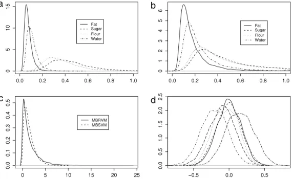
Fig. 3. Biscuit dough composition data set. The 4 components are fat, sugar, flour and water. (a) Distribution of MSEP for the 4 components of biscuit dough under MBRVM model. (b) Distribution of MSEP under MBSVM model. (c) Posterior distribution of the kernel parameterθunder MBRVM and MBSVM models. (d) Posterior distribution of the correlations under MBRVM models.

9. Concluding remarks

The RKHS based SVM and RVM methodology turns out to be a strong contender for prediction. Specially, in the cases where we have a very large number of covariates but very small amount of data, its performance does not deteriorate with high input dimensionality. Unlike other machine learning methods, our models do not require an additional projection into sample space. Indeed, the dimension reduction is built automatically in the SVM and RVM methodology, as by Wahba’s representation we are reducing the dimension frompton. Mallick et al. [14] introduced Bayesian SVM for binary classification with the hinge loss function. SVM for classification is well studied due to its immediate applicability in disease/tumor classification based on microarrays. However, SVM for regression under Bayesian framework is not very well studied. In this paper we developed a mixture distribution representation for the Vapnik’s

ϵ

-insensitive loss for regression problems and extended it to the multivariate set up. When the response is multivariate the prediction or modeling the dependency is challenging. In this paper we have proposed to model the underlying dependency of the correlated response through latent variables. Our models can predict the whole response vector together. Additionally, we have also introduced an empirical Bayes formulation of our multivariate Bayesian SVM and RVMs. The empirical Bayes formulation was not considered in [14].

The results from the life example and the simulated data set give strong credence to the view that our RKHS based Bayesian SVM and RVM help to build a much stronger learning algorithm than other straightforward methods like partial least square, principal component regression and stepwise multiple linear regression. It also performs much better than some very sophisticated methods like Bayesian wavelet regression of Brown et al. [6] and Bayesian decision theory approach of Brown et al. [5]. Our MBSVM also has its virtues over the classical support vector machine by producing a richer class of models which give better prediction along with the unique ability to quantify the prediction error, i.e., now we can have the entire posterior distribution of MSEP and can obtain a confidence interval (Fig. 3). Rather than having just a point predictor now we can have the full posterior predictive probability distribution of a future observation. The results fromTables 1and

2indicates the success of our MBSVM method in handling outliers in the data set. The MSEP, specially in the sugar and flour component remains not very affected in the robust loss function based MBSVM model as compared to the MBRVM model which is based on the squared error loss function. This is good in terms of the robustness point of view.

In the studied biscuit dough data the improvement of our MBRVM and MBSVM over competing models is more pronounced, where the MSEP reduction ranges between 8% and 31%. Empirical Bayes RVM and SVM has their own advantages and disadvantages. In terms of prediction accuracy it comes close but inferior to the hierarchical Bayes models. But adopting an empirical Bayes approach, one can avoid some prior elicitation problems. Choice of multiple smoothing parameters has a distinct advantage over the single smoothing parameter. Apart from the fact multiple smoothing parameters provide independent shrinkage for the components of regression coefficients and result in sparsity, it gives better prediction. Thus, overall our recommendation is to use either hierarchical Bayes multivariate RVM (MBRVM) or hierarchical Bayes multivariate SVM (MBSVM) with multiple smoothing parameters for ‘‘largepsmalln’’ regression problems.

(13)

Table 4

Average mean squared errors of prediction from 20 randomly split biscuit data sets. The number in parenthesis is the standard deviation of MSEP.

Stepwise MLR 0.412 (0.037) 2.831 (0.409) 2.910 (0.416) 1.002 (0.130) Decision theory 0.281 (0.023) 1.059 (0.171) 0.899 (0.065) 0.606 (0.031) PLS 0.416 (0.032) 1.209 (0.161) 1.352 (0.175) 0.811 (0.043) PCR 0.432 (0.041) 1.176 (0.182) 1.461 (0.172) 0.921 (0.065) BWR 0.203 (0.019) 0.714 (0.027) 0.913 (0.033) 0.629 (0.017) CSVM-P 0.403 (0.031) 1.132 (0.140) 1.222 (0.164) 0.632 (0.033) CSVM-G 0.511 (0.057) 1.528 (0.165) 1.399 (0.189) 0.819 (0.060) Hyperparameter choice (i)

MBRVM 0.133 (0.022) 0.723 (0.041) 0.789 (0.057) 0.519 (0.025) MBSVM 0.139 (0.023) 0.811 (0.030) 0.862 (0.061) 0.515 (0.040) EMBRVM 0.168 (0.032) 0.884 (0.052) 0.809 (0.063) 0.510 (0.037) EMBSVM 0.189 (0.037) 0.861 (0.072) 0.803 (0.065) 0.496 (0.048)

Acknowledgments

The research of Bani K Mallick was supported by National Science Foundation grant DMS 0914951 and by award KUS-CI-016-04 made by King Abdullah University of Science and Technology (KAUST).

Appendix

In this section we provide some additional data analysis. We merge the original training and test set of the biscuit data and then randomly split into training and test (39 in training and 39 in test) for 20 times and calculate the MSEP and their standard deviations over those 20 random splits. The results corresponding to these 20 random splits are reported in

Table 4.

References

[1] D.F. Andrews, C.L. Mallows, Scale mixtures of normal distributions, Journal of the Royal Statistical Society, Series B 36 (1974) 99–102. [2] N. Aronszajn, Theory of reproducing kernels, Transactions of the American Mathematical Society 68 (1950) 337–404.

[3] J.M. Bernardo, A.F.M. Smith, Bayesian Theory, Wiley, London, 1994.

[4] C. Bishop, M. Tipping, Variational relevance vector machines, in: C. Boutilier, M. Goldszmidt (Eds.), Proceedings of the 16th Conference in Uncertainty and Artificial Intelligence, Morgan Kauffman, 2000, pp. 46–53.

[5] P.J. Brown, T. Fearn, M. Vannucci, The choice of variables in multivariate regression: a Bayesian non-conjugate decision theory approach, Biometrika 86 (1999) 635–648.

[6] P.J. Brown, T. Fearn, M. Vannucci, Bayesian wavelet regression on curves with application to a spectroscopic calibration problem, Journal of the American Statistical Association 96 (2001) 398–408.

[7] S. Chib, E. Greenberg, Understanding the Metropolis–Hastings algorithm, The American Statistician 49 (1995) 327–335.

[8] A. Gelfand, A.F.M. Smith, Sampling-based approaches to calculating marginal densities, Journal of the American Statistical Association 85 (1990) 398–409.

[9] I.J. Good, The Estimation of Probabilities. An Essay on Modern Bayesian Methods, MIT Press, MA, 1965. [10] P. Huber, Robust estimation of a location parameter, Annals of Mathematical Statistics 53 (1964) 73–101.

[11] G. Kimeldorf, G. Wahba, Some results on Tchebycheffian spline functions, Journal of Mathematical Analysis and Applications 33 (1971) 82–95. [12] M.H. Law, J.T. Kwok, Bayesian support vector regression, in: Proceedings of the Eighth International Workshop on Artificial Intelligence and Statistics,

AISTATS, Key West, Florida, USA, 2001, pp. 239–244.

[13] D.J.C. MacKay, Bayesian non-linear modelling for the prediction competition, ASHRAE Trans. 100 (21) (1994) 1053–1062.

[14] B.K. Mallick, D. Ghosh, M. Ghosh, Bayesian classification of tumors using gene expression data, Journal of the Royal Statistical Society, Series B 67 (2005) 219–232.

[15] C.E. McCulloch, Maximum likelihood algorithms for generalized linear mixed models, Journal of the American Statistical Association 92 (1997) 162–170.

[16] N. Metropolis, A.W. Rosenbluth, M.N. Rosenbluth, A.H. Teller, E. Teller, Equations of state calculations by fast computing machines, Journal of Chemical Physics 21 (1953) 1087–1092.

[17] R.M. Neal, Bayesian Learning for Neural Networks, Springer-Verlag, New York, 1996.

[18] B.G. Osborne, T. Fearn, A.R. Miller, S. Douglas, Application of near–infrared reflectance spectroscopy to compositional analysis of biscuits and biscuit doughs, Journal of the Science of Food and Agriculture 35 (1984) 99–105.

[19] E. Parzen, Statistical inferences on time series by RKHS methods, in: Proceedings of the 12th Biennial Seminar, Canadian Mathematical Congress, Montreal, Canada, 1970, pp. 1–37.

[20] P. Sollich, Bayesian methods for support vector machines: evidence and predictive class probabilities, Machine Learning 46 (2001) 21–52. [21] M. Tipping, The relevance vector machine, in: S. Solla, T. Leen, K. Muller (Eds.), Neural Information Processing Systems—NIPS, vol. 12, MIT Press,

Cambridge, MA, 2000, pp. 652–658.

[22] M. Tipping, Sparse Bayesian learning and the relevance vector machine, Journal of Machine Learning Research 1 (2001) 211–244. [23] V.N. Vapnik, The Nature of Statistical Learning Theory, second ed., Springer, New York, 1995.

[24] G. Wahba, Spline Models for Observational Data, SIAM, Philadelphia, 1990.

[25] G. Wahba, Support vector machines, reproducing kernel Hilbert spaces and the randomized GACV, in: B. Schölkopf, C. Burges, A. Smola (Eds.), Advances in Kernel Methods, MIT Press, Cambridge, MA, 1999, pp. 69–88.

[26] G. Wahba, Y. Lin, Y. Lee, H. Zhang, Optimal properties and adaptive tuning of standard and nonstandard support vector machines, in: D. Denison, M. Hansen, C. Holmes, B. Mallick, B. Yu (Eds.), Nonlinear Estimation and Classification, Springer, New York, 2002, pp. 125–143.

Journal of Multivariate Analysis 108 (2012) 28–40

SciVerse ScienceDirect