Reservoir computing with output feedback

(1)

Reservoir Computing

with Output Feedback

Ren´e Felix Reinhart

Vorgelegt zur Erlangung des akademischen Grades

Doktor der Naturwissenschaften

Technische Fakult¨

at, Universit¨

at Bielefeld

Oktober 2011

(2)

(3)

Abstract – Reservoir Computing

with Output Feedback

Ren´

e Felix Reinhart

A dynamical system approach to forward and inverse modeling is proposed. Forward and inverse models are trained in associative recurrent neural networks that are based on non-linear random projections. Feedback of estimated outputs into such reservoir networks is a key ingredient in the context of bidirectional association but entails the problem of error amplification. Robust training of reservoir networks with output feedback is achieved by a novel one-shot learning and regularization method for input-driven recurrent neural networks. It is shown that output feedback enables the implementation of ambiguous inverse models by means of multi-stable dy-namics. The proposed methodology is applied to movement generation of robotic manipulators in a feedforward-feedback control framework.

Keywords: forward and inverse models, bidirectional association, recurrent neural networks, output feedback dynamics, regularization, stability

(4)

(5)

Introduction

Association is a key principle of neural processing [1, 2, 3]. An associative connection between two entities is naturally bidirectional, and, as a process, denotes the recall of one entity from the other. Many connectionist models of associative memory have been developed [4, 5, 6, 7]. Despite their ability to learn from examples and their neuroscientific motivation, early compu-tational models of associative memory have rather limited capabilities: Hopfield-type networks [4] can associate only a discrete number of patterns with each other and fail to generalize to continuous mappings. Then, associative computation remains a neural model of content ad-dressable memory. In the context of bidirectional association, another challenge arises that is rarely discussed but important to the subject: If the forward relation is many-to-one, the reverse relation is ambiguous, i.e. one-to-many. In terms of continuous mappings, the forward mapping is not invertible.

The case of ambiguous inverse models is a common problem in many application areas ranging from control engineering to computer vision. For instance, recognizing objects and their spatial orientation is an one-to-many mapping due to loss of information when three-dimensional scenes are projected onto a two-three-dimensional retina. Kersten therefore coined the term ”inverse graphics” for object recognition [8]1. Hinton also emphasized the need for both, internal forward and inverse models, in [10] where he proposed “to recognize shapes, first learn to generate images”. In linguistics and functional neuroanatomy of language, it has been stated that speech recognition is the inverse process of speech production [11, 12]: The listener es-timates configurations of the vocal tract from auditory input, which is an ambiguous inverse relation. The requirement of solving forward and inverse problems is even more prominent in motor learning. It has been hypothesized that paired forward and inverse models are crucial for skilled movement generation [13]. In particular, human reaching performance in the absence of visual feedback and also delayed proprioceptive feedback strongly indicate the presence of internal forward and inverse models in the brain [14]. Redundancy of the movement apparatus further gains ambiguity of the inverse model. The ambiguity of one-to-many relations states a main problem in these contexts.

In principle, the problem of ambiguity can be approached following one of two paradigms: Either, ambiguous data samples are discarded and learning is restricted to a single solution [9, 15, 16, 17]. Or, ambiguity is represented by a model such that multiple solutions to the inverse problem coexist [18, 19, 20, 21]. On the one hand, restricting the inverse model to a single solution alters the original one-to-many relation to a simpler one-to-one mapping which can be learned with classical feed-forward networks. On the other hand, this restriction renders the inverse model incomplete in the sense that not all possible solutions are captured by the model. The restricted modeling of a single solution only is often not appropriate. For instance,

1_{Even earlier, Poggio}_{et al.} _{denoted early vision to be “inverse optics“ [9].}

(8)

2 Introduction

consider inverse graphics where modeling of a single solution rejects possibly correct solutions.

Fig. 1.1: The Necker cube admits ambiguous interpre-tation of its spatial configu-ration.

The multiplicity of the inverse relation adds flexibility to a system which is often more meaningful than apriori selection of a single response. However, representing one-to-many relations entails additional problems like the selection of a particular solu-tion during system exploitasolu-tion. The commitment to a particular solution out of many, i.e. ambiguity resolution, is often accom-plished by additional circuitry [18, 13]. A more natural approach to ambiguity resolution is to utilize additional information that is integrated over time. For example, consider following the mo-tion of an object for a while to disentangle if it is moving towards or away from you. An internal representation then “stands in“ [14] for the missing information from the sensory input which has been hypothesized to be a minimal requirement for a system to be cognitive. A simple example for the resolution of ambiguity

by an internal representation is the Necker cube (see Fig. 1.1). One perceives either one face to the front or the other depending on which information the perceiver adds internally to the same sensory stimulus. Essentially, the combination of forward and inverse models, memory and learning by means of bidirectional association constitutes a key ingredient of cognition.

In this thesis, the associative principle is revived by an adaptive dynamical system approach that facilitates bidirectional and continuous association of ambiguous mappings. I combine and extend previous ideas to efficient training of connectionist models proposed in [22] and [23, 24] to achieve robust learning of bidirectional associative models. Inputs and outputs are treated as parts of a larger recurrent neural network with a hidden layer. Continuous association is modeled as an input-driven process, i.e. the system’s representation is continuously biased by external inputs. Inputs or outputs are driven on demand in order to approximate the forward or inverse relation. The network dynamically inserts estimated values for the unspecified network parts in a recursive feedback loop. These feedback dynamics of estimated outputs can be multi-stable and thereby represent one-to-many relations. I formalize the concept of feeding back estimated outputs under the notion of output feedback dynamics. This concept unifies the ideas applied in a range of connectionist models, e.g. feed-forward networks with additional recurrent loops [25, 26, 20, 27, 28], fully recurrent neural networks [29] and particular flavors thereof [30, 22, 31, 23]. Ambiguity resolution by output feedback dynamics is based on the current system state that acts as short-term memory and integrates the internal representation over time.

An early and conceptually similar approach dates back to Barhenet al. [29]. They proposed an attractor-based scheme for learning inverse kinematics of redundant robots. In the outset of their method, multiple solutions of the inverse kinematics are represented by multi-stable attractor dynamics. Learning adapts all weights to imprint the training data into such attrac-tor dynamics. The approach therefore suffers all the standard problems with complexity and efficiency of recurrent network training [32], and – while conceptually elegant – has not been demonstrated to be usable in practice for real robot applications.

Another related approach to represent multi-valued functions in a dynamical network has been proposed in [20]. Tomikawa and Nakayama utilize a combined representation of inputs and outputs in the hidden layer of a feed-forward network in order to resolve the ambiguity of multi-valued functions for learning. During system exploitation, estimated outputs are fed back iteratively into the network very similar to the model that is proposed in this thesis. How-ever, additional constraints, in particular an integral condition, added to the learning objective renders training inefficient despite the feed-forward network structure. Moreover, weights of the additional constraints have to be balanced precisely [20], which makes learning sensitive to parameter configurations, and the model was only applied to toy examples.

(9)

3

I follow another thread of research that considers non-linear random projections networks. A basic variant of these networks was introduced under the notion of extreme learning ma-chines [33]. Their spatio-temporal siblings comprise additionally random feedback connections between hidden processing units which provide a “rich reservoir” of dynamics [34]. These so called reservoir computing networks support efficient learning and obviate tuning of the inter-nal representation. Bidirectiointer-nal association in these reservoir networks is based on training a perceptron-like read-out layer which is recurrently connected to the reservoir. Training of the read-out connections imprints desired relations between inputs and outputs into the otherwise untrained network. In this thesis, associative reservoir computing networks with output feed-back dynamics are trained to model forward and – possibly ambiguous – inverse relations. The success of the proposed approach requires the integration of learning and input-driven dynam-ical systems, which is particularly challenging with respect to stability of the output feedback dynamics. Feedback of erroneous outputs into the network can lead to error amplification which is a serious problem. Although output feedback dynamics and the associated stability problem occurs also in related connectionist models [25, 26, 20, 29, 27], stability of the output feedback dynamics is rarely discussed, e.g. in [35]. I formalize the concept of output feedback dynamics and the connected problem of output feedback stability in this thesis.

In the context of bidirectional association, another problem arises. Externally driven net-work parts change depending on which relation is currently queried, e.g. driving inputs while estimating outputs or vice versa. It is important to balance the contribution of inputs and out-puts to the network such that the network state can equally well be driven by inout-puts or outout-puts. Otherwise, either the forward or inverse relation is modeled primarily and bidirectionality of the model is compromised.

I approach these crucial issues in the context of reservoir computing with output feedback in three steps. I first formalize the concept of output feedback dynamics and propose a tai-lored output feedback stability criterion. In a second step, I show that regularization of the learning and the internal representation mitigates the stability issue to a great extent. While regularization of the learning has been previously shown to support stability [36, 35], regular-ization is extended to the internal representation in this thesis. The main idea of this reservoir regularization is to implement desired network dynamics with small weights which reduces the gain of the system. For this purpose, I propose an efficient one shot learning method for input-driven recurrent neural networks that combines ideas from reservoir computing and associative memories. The reservoir regularization method increases the robustness of learning success by stabilizing output feedback dynamics. With the same methodology, also the problem of balanc-ing contributions to the hidden layer is resolved in a sbalanc-ingle step. Stability of the output feedback dynamics and the balancing of contributions are necessary prerequisites for the application of reservoir networks with output feedback to bidirectional association.

With these concepts and methods at hand, I tackle the problem of ambiguity in a third step. I first show that ambiguity can be resolved by output feedback dynamics. I then adopt the developed one-shot learning methodology to shape multi-stable output feedback dynamics of the recurrent network model. Multi-stable output feedback dynamics represent one-to-many relations and disentangle ambiguous sensory stimuli by means of a short-term memory. I eval-uate properties of the multi-stable attractor dynamics and demonstrate their application in different scenarios.

Finally, the gathered techniques are applied to movement generation, which is a salient example for forward and inverse modeling in the context of motor learning. In robotic experi-ments, I show that the proposed model for bidirectional association performs smooth movement generation in a feedforward-feedback control loop. The presented results emphasize the com-putational power of bidirectional association with dynamical systems. This thesis essentially contributes to the robust and efficient learning of bidirectional and ambiguous relations in dy-namical connectionist models.

(10)

Chapter 2

Associative models, inverse problems

and ambiguity

In this chapter, mathematical prerequisites concerning association, continuous mappings and inverse problems are introduced. A brief review of associative models is given along the discus-sion and the methodology developed in this thesis is related to state-of-the-art approaches. At the end of this chapter, Tab. 2.1 gives a compact overview of the discussed associative methods.

2.1

Bidirectional association

Consider a set of data pairs_{(xn,yn)}n=1,...,N, wherex∈RD andy∈RO. Association denotes

the process of recalling the corresponding output pattern yn given a probably corrupted input

pattern xn+ν [37, 7]. Association of patterns with themselves, i.e. xn ≡ yn, is called

auto-association and hetero-auto-association otherwise. More formally, auto-association is a relation

f :X⊂RD →Y ⊂RO

with a finite domain,_|X_|<_∞(see Fig. 2.2 (left)). Training samples (xn,yn) strictly define the

associative relation f only for a finite set. In the recalling phase, inputs are generally drawn from the entire input space.

Standard Hebbian, correlation-based or pseudo-inverse learning can be employed to form linear transformations from the input space to the output space such that output patterns can be “retained” from an input key by a simple matrix multiplication [38, 7, 37]. Theseassociative memory (first row in Tab. 2.1) models store the output data in their model parameters in a distributed fashion [38, 37, 7]: The input data and the fitted model are sufficient to recall

yn from xn for n = 1, . . . , N. In case of correlation-based learning and orthogonal input

patterns, all output patterns can be correctly recalled [38, 7]. For pseudo-inverse learning, linear independence of the input patterns is sufficient to achieve perfect recall [37].

The scheme of associative recall has been generalized to non-linear and dynamic associative memory models. The underlying principle of dynamical associative memories, such as the auto-associative Hopfield network [4] and its hetero-auto-associative generalization [5], is the convergence of feedback dynamics to a fixed-point depending on the initial condition. Learning is supposed to shape the dynamics such that training patterns reside in the center of attractor basins. Iterating the dynamics from any initial condition in the attractor basin of a training pattern results in the recall of this pattern. I.e. dynamical associative memories robustly recall stored patterns from noisy keys which is often emphasized to be a desirable feature [37, 4, 5]. However, this paradigm drastically affects the kind of computation that can be accomplished: Association of discrete patterns enables robust recall in the presence of noise. But the gained robustness of 4

(11)

Forward and inverse models 5

Fig. 2.2: Association: Mapping a finite domain to its codomain (left). Bidirectional association additionally maps the finite codomain back to its domain. Injective mapping shown.

saddle nodes input x o ut put y x y 1 1 xn yn

Fig. 2.1: Associative memories are piecewise constant, discontin-uous functions.

recalling a finite set of patterns limits generalization of net-work responses to novel inputs. Through the glasses of func-tion approximafunc-tion, these associative models implement a piecewise constant, “quantized” [39] function with disconti-nuities at the borders between attractor basins (see Fig. 2.1). Discontinuities are typically due to saddle nodes of the dy-namics, i.e. instable fixed-points, at the border of two at-tractor basins (circles in Fig. 2.1). The associative memory function f is queried at novel inputs and recalls the associ-ated training patterns in the output space. Generalization by means of inter- or extrapolation is therefore restricted. Typical applications of discrete association are content ad-dressable memories and pattern recognition. Also, sequence generation can be implemented by auto-association of pat-terns at successive time steps, i.e. x(k+1) =f(x(k)) [37, 4, 5].

Given a set of data pairs {(xn,yn)}n=1,...,N, there is apriori no meaningful difference in

associating inputs from outputs or vice versa. Kosko therefore proposed to bidirectionally associate “inputs“ with “outputs” [5]. His bidirectional associative memory (BAM, second row in Tab. 2.1) subsumes the Hopfield network as a special case and can be further generalized to multi-directional associative memories [40, 41]. The bidirectional association of finite sets is illustrated in Fig. 2.2 (right).

Most of the discussed associative memory models can be generalized to the case of multi-directional association. An early approach to multi-multi-directional association, the Associatron [42] introduced by Nakano in 1972, comprises an internal representation in addition to input and outputs. Nakano formulated the concept of associative memories with multiple “neural areas” [42] to increase the memory capacity and resolve the problem of cross-talk between patterns. In this thesis, the coupling of multiple representations by an internal representation is also pursued. I focus on the case of input, internal and output “fields“ only, which is sufficient for the discussion and does not impair the generality of the approach.

2.2

Forward and inverse models

In many cases, there is a continuous regularity between inputs and outputs which shall be extracted by learning of a parameterized model. Continuity means that a small change in input space corresponds to a small change in the output space, i.e. f(xi) ≈ f(xj) if xi ≈ xj (see

Fig. 2.4). Approximating a continuous mapping f :X _→Y with_|X_|=_∞ by a parameterized model then enables to generalize the relation of inputs and outputs in the data to novel inputs that are not part of the training data.

Similar to the generalization of associative memories to bidirectional association, modeling the forward mapping f :x_7→y is not different from modeling the inverse mappingg :y_7→ x

under certain conditions. Formally, g is a right inverse of f if (f ◦g)(y) =y ∀y ∈ Y. Note that a right inverse g may map outputs y to any x with f(x) = y. That is, the right inverse

(12)

6 Associative models, inverse problems and ambiguity

Fig. 2.4: Continuous and invertible mapping mapping (left). Bidirectional mapping with multi-valued and continuous inverse (right).

is not necessarily unique. The inverse is unique if g is also the left inverse of f such that (g◦f)(x) = x ∀x ∈X holds for the reverse composition. It is useful to distinguish different properties of the forward mapping in order to determine uniqueness or ambiguity of the inverse: Iff is a homeomorphism, i.e. f is a continuous and bijective mapping, the forward mapping is invertible. Then, the forward and inverse mappings are both unique and continuous (sometimes referred to as one-to-one, see Fig. 2.4 (left)).

branch principle branch output y inpu t x

Fig. 2.3: Forward and inverse function with multiple solution branches.

In many cases, however, the forward mapping is not in-jective and thus not invertible. This is always the case if there exist several causes that result in the same effect, e.g. several joint angles can result in the same end effector posi-tion. Then, the inverse relation is ambiguous (also referred to as one-to-many). Formally, there exist several functions

gb with f(gb(y)) = y that are defined on a subset of the

codomain of f and are called solution branches. Typically, there is a principle branch g that is defined on the entire codomain off(see Fig. 2.3). Note that continuity may apply to each of the solution branches setting up multiple smooth solution manifolds (see Fig. 2.4 (right)). Solving this in-verse problem, i.e. providing one of many suitable inputs to obtain desired outputs, is important in various application domains ranging from control engineering [15] to pattern recognition [9, 8].

From a set-theoretic viewpoint, the inverse of a non-injective function is a multi-valued functionf :y_{7→ {}xb}b=1,...,B. In Fig. 2.5 (left) the multi-valued relation between outputs and

inputs that stems from a non-injective forward model is illustrated using sets. Typically, the set of solutions for all outputsyis non-convex unless the forward mapping is not constant for a range of inputs x. In other words, the set of solutions _|{xb}|<∞ is discrete and thus forms a

non-convex subset in the continuous input spaceX. Constant forward mappings have infinitely many inverse solutions. That is, the multi-valued inverse function has an infinite codomain (_|{xb}|=∞). This set of solution can in addition be non-convex, e.g. if two spatially separated

regions of the input space map to the same output value. In general, there are complex relations between sets in both spaces, including overlaps and inclusions. A fork of branches, for instance, translates into ”adjacent” sets, because the point of bifurcation belongs to both branches (or to the principal branch only depending on the definition). Fig. 2.5 (right) and Fig. 2.3 finally show that cases exist where both, the forward and the inverse relation can be ambiguous. Note that noisy data in practice compromise the uniqueness of the forward mapping: Probing outputs for the same input several times yields to various observations due to noise and thus the forward mapping is, strictly speaking, not one-to-one even though the function underlying the data generation process is an one-to-one mapping.

Although there is apriori no preferred direction of mapping “inputs“ to “outputs” or vice versa, the process underlying the generation of inputs and outputs is often causal. For instance, consider the causal relationship between joint angles and the resulting end effector position

(13)

Inverse problems and ambiguity resolution 7

Fig. 2.5: Multi-valued inverse relation (left): Multiple values of the inverse are due to a non-injective forward mapping. Also both, the forward and inverse relation, can be multi-valued (right). Ambiguous relations are indicated by dashed arrows.

of a manipulator. Causality in physical systems induces directionality of the relation between inputs and outputs. Then, an approximation off is typically referred to asforward model which maps causes to effects. Modeling g is denoted as inverse modeling accordingly. In this thesis, adaptive bidirectional mappings by means of combined forward and inverse models are the core application theme.

The terminology above also generalizes to the case of time-series data. Temporally ordered data samples, i.e. time-series, are indicated by sample indices k in parentheses, x(k). In this thesis, smooth trajectories, i.e. x(k+ 1) _≈ x(k), and a continuous forward mapping are typically considered. For instance, consider data to be collected along the trajectories shown in Fig. 2.4. The mapping of sequencesx(k) toy(k) is generally denoted bysequence transduction. Analogously, bidirectional sequence transduction is the combined forward and inverse mapping of time-series.

2.3

Inverse problems and ambiguity resolution

In case of a non-injective relation between inputs and outputs, there is no unique solution to the inverse problem. For instance, in the context of control engineering multiple system inputs can cause the same system state and thus there are multiple solution branches to the inverse problem. How can the problem of ambiguity be tackled? How can multiple solutions be represented, and how to select a solution, i.e. how to resolve ambiguities?

From a machine learning perspective, multiple solutions to an inverse problem constitute a serious problem for traditional feed-forward function approximators. Consider ambiguous data pairs (xn,yn) and (xm,ym) with xn=xm and yn6=ym for n 6= m. Ambiguous data pairs

with the same or similar input but distinct outputs result in averaged approximations: Any feed-forward model is a function f : x _7→ y that maps inputs to unique outputs. Parameter estimation from ambiguous data pairs fails due to the non-convexity of many inverse problems, i.e. typically the least squares solution 1₂(yn +ym) does not necessarily reside in the

non-convex solution set (compare Fig. 2.3 and the discussion in [15, 26]). Note that the problem is due to the fact that the input representation is the same for both outputs and thus does not allow to discriminate between solutions. Traditional feed-forward architectures can therefore not represent multiple solutions to a mapping without additional knowledge.

In the following, main learning approaches that tackle the inverse problem are discussed. 2.3.1 Restricted inverse modeling

The first approach restricts modeling to a single solution by assuming that the training data comprises samples of only a particular, e.g. the principle, solution branch of the inverse problem. This restriction converts the original ambiguous problem into a unique mapping task. Solving the inverse problem is shifted to the data collection process. It is, however, not trivial to decide if data stems from a single solution to the inverse problem or how to obtain data for a single solution only. This problem has been approached from different directions.

(14)

In [15], a distal teacher formulation for a composite setup comprising a serial combination of an inverse and forward model has been proposed. Training the inverse model is based on gradient descent with respect to the performance error mediated through the forward model. The performance errorf(g(y))−yis evaluated in target space, e.g. yis the desired end effector position of a robot arm. Thereby, a particular solution to the inverse problem is found and the non-convexity problem is circumvented (see [15] for a decent discussion). Selection of a particular solution depends on initial conditions, exploration of control commands and can be biased by introducing additional costs to the error function.

In [43, 44], the non-convexity problem is solved by utilizing a strong bias of the model, i.e. a topological arrangement of neurons in a self-organizing map, which results in selection of a single solution branch of the inverse problem. The original variant ofself-organizing maps(SOM, third row in Tab. 2.1) is closely related to vector quantization and the local representation of inputs in the model restricts its generalization abilities. This drawback is cured by the “continuous generalization” of the self-organizing map [16]. Theparameterized self-organizing map (PSOM, fourth row in Tab. 2.1) approximates a continuous manifold by utilizing basis functions that areparameterized by the underlying grid of local prototypes. A review of self-organizing maps and in particular their application to modeling inverse problems can be found in [39].

A goal-directed inverse modeling approach is taken in [17] which solves the non-convexity problem during control space exploration. “Goal babbling“ [17] utilizes the structure of the goal-directed exploration process to weight collected data samples in order to resolve ambiguities of the inverse problem. Also this approach alleviates the non-convexity problem for the learner, which therefore can be any feed-forward function approximator.

Strong biases either of the model or by means of constrained learning [9, 26, 45] are typical approaches to cope with ill-posed inverse problems. However, a main drawback of restricting the inverse model to a single solution branch is that the inverse model is not complete. That is, the inverse model provides only a subset of the multi-valued inverse function. Moreover, the selected solution is either depending on initial conditions or is biased by incorporating prior knowledge.

2.3.2 Combining multiple experts

A second approach to deal with ambiguous inverse problems is to model each solution manifold separately, i.e. learning a set of expert models [18]. Solution selection during system exploitation then reduces to selection of an expert model that models a specific branch of the inverse.

This modular approach can be understood as generalization of the previous approach to select a specific solution to the inverse problem per model and hence inherits some of its diffi-culties: It is difficult to assign data samples to models such that each expert is trained with data from a single solution branch [18]. It is also apriori unclear how many expert models are needed to model the complete inverse problem, i.e. how many solution manifolds exist. And finally, an external gating or responsibility model has to be trained that selects an expert depending on the current control task [18, 13, 46, 47]. Though arbitrary criteria could be implemented here independently of the inverse models, it is an additional burden to design such a gating. Moreover, a discrete set of experts can not model a continuous set of solutions, which occurs always if the forward mapping is constant in a region of the input space.

A variant of the expert model approach represents multiple solutions in a single model with additional inputs [21]. The additional inputs parameterize the learner’s representation, alleviate the non-convexity problem during learning, and serve as selection mechanism during exploitation [48, 15]. This approach inherits the same drawbacks as the expert modeling approach and also requires supervised assignment of data pairs to particular input parameter configurations.

(15)

2.3.3 Recover invertibility by augmenting the inverse problem

Another approach tackles ambiguous inverse problems by adding augmented variables to the input data which resolve the ambiguity. The augmented variables act as additional constraints that select/discard particular solutions in the set of inverse solution branches. This approach is related to the previously discussed approach to parameterize the inverse model for the selection of sub-models. It is nevertheless useful to distinguish parameterizing a model in a rather binary fashion to select expert models from introducing augmented variables that resolve ambiguity by means of intrinsic properties of the inverse function. In the latter case, ambiguities are resolved by means of additional, typically domain-specific, constraints to the inverse model.

For instance, the model presented in a series of papers [49, 50, 51] implements feedback dynamics based on the mean value of multiple computations (MMC, fifth row in Tab. 2.1). In MMC networks, redundant sets of equations are provided by the designer which represent partial aspects of the modeled system. Ambiguity is resolved by augmenting the core relation between inputs and outputs with additional equations that, for example, express some constraints. Dur-ing network exploitation, estimated variables are averaged over all redundant equations and then again fed back into the equations. These MMC dynamics relax to a particular solution even if the input does not fully constrain the solution, i.e. the approach copes with infinitely many solutions to the inverse problem.

In [16], a parameterized self-organized map was trained on augmented data which then al-lowed to resolve the ambiguous inverse kinematics of a simulated three link, four degrees of freedom robot arm. The augmented variables express specific constraints of the inverse model, e.g. coupling between joint angles or the elevation of a particular link, that can be weighted flexibly during model exploitation. In an expert model approach, this is not possible with-out knowledge abwith-out the particular properties of each expert. However, defining augmented variables requires even more complex domain knowledge of the inverse problem than assigning solution branches to expert models. Also, the selection of a particular solution during exploita-tion by means of selecting values for the augmented variables is left to addiexploita-tional mechanisms in this scheme.

2.3.4 Recover invertibility by incorporating temporal context

A fourth approach exploits temporal context to decide between ambiguous control schemes. For instance, originally instantaneous inverse problems are turned into a spatio-temporal mapping. But there are also inverse problems that naturally reside in the temporal domain. The resolution of ambiguities is then based on the history of inputs, i.e. memory. Memory in connectionist models is typically modeled by time delay lines [25] or transient-based short-term memories [52]. This scheme of ambiguity resolution is only meaningful in case of temporally correlated data and can be understood as temporal variant of the augmented variables approach. In deed, traditional neural time-series classification approaches consider learning as internal representation pursuit [25] and face the problem of typically ambiguous, non-discriminative input samples withx(k1) =

x(k2) but y(k1)6=y(k2) for some k16=k2.

In this thesis, I also consider ambiguous time-series data pairs but which stem from a static relation between inputs and outputs. That means the data is temporally ordered but the un-derlying relation is instantaneous and requires no memory of the history: y(k) =f(x(k)). For instance, let x(k) be the joint angle configuration of a manipulator and y(k) the end effector position. Then, using augmented variables that encode the temporal history has the drawback that different temporal dynamics of the inputs, i.e. speeds, disturb the spatio-temporal rep-resentation and thus can deteriorate the inverse model. Normalization of the data, e.g. by temporal warping of input sequences, or learning from rich data sets comprising several se-quences with exemplary speeds becomes necessary and introduces additional costs. I show in Chapter 7 that an attractor-based approach to memory circumvents these problems.

(16)

2.3.5 Modeling inverse problems with probabilistic methods

Probabilistic methods have been applied to solve ambiguous inverse problems, e.g. [53]. Ba-sically, the non-convexity problem is approached by modeling the joint distribution P(x,y) of inputs and outputs. Then, given a particular input x, the conditional distribution P(y|x) provides a possibly multi-modal distribution of outputs. Also direct models of the conditional densityP(y_|x) can be learned which circumvents modeling the joint distribution, e.g. [54].

However, density estimation in high-dimensional spaces is notoriously hard and requires many training samples which are typically costly to collect. Moreover, the problem of explicitly selecting a particular output, i.e. a solution, from a multi-modal distribution remains. A maximum a-posteriori estimate is a good choice in general, but the value that maximizes the posterior could flip between two modes for small changes of the input. Also in the case of infinitely many solutions that cause a plateau of the posterior distribution, it remains an open question how to select a particular solution.

2.3.6 Dynamical system approach to inverse modeling

In this thesis, another approach is pursued that combines a joint representation of inputs and outputs with a dynamical ambiguity resolution scheme. The non-convexity of ambiguous in-verse problems is tackled by utilizing a joint representationh(x,y) of inputs and outputs in a connectionist model. I.e. an internal representation h(x,y) is formed that is uniquely defined byx andy (compare Fig. 2.7 (left)). Learning a mapping fromh(x,y) to eitherx ory is then unique and does not suffer from the non-convexity problem becauseh(xn,yn)6=h(xm,ym) also

ifxn=xm and onlyyn6=ym forn6=m.

saddle node manifold fork/ merge flip driving input o ut put f ee dba ck dyna mics x y(k) y(k+1)

Fig. 2.6: Dynamical system approach to in-verse modeling: Multiple attractor mani-folds with typical bifurcations.

During network exploitation, typically only the input x is available and an appropriate output y

shall be estimated by the model. Thus, the joint representation can not be calculated directly. The idea is to iteratively approach the joint represen-tationh(x,y) givenx only by means of an input-driven, dynamical process using the current esti-mate ofy(k) at iteration stepk. Based on the cur-rent internal representationh(x,y(k)), the output

y(k+1) at the next time step is computed which is then recursively fed back into the model (com-pare Fig. 2.7 (right)). Learning in this framework reduces to assuring thaty(k+1) is closer to the de-sired outputythany(k). Then, theseoutput feed-back dynamics give a slightly improved estimate

y(k+1) and eventually converge toy. That is, the output y is associatively recalled from inputx by

approaching an attractor of the possibly multi-stable output feedback dynamics. The driving input x continuously parameterizes the points of attraction of the output feedback dynamics. This enables the approximation of continuous mappings by means of parameterized attractor manifolds (see Fig. 2.6) which is fundamentally different from the piece-wise constant functions approximated by traditional associative memories.

Output feedback dynamics can be multi-stable [20, 31, 55], i.e. have several points of attraction for each input x. Solution branches of an ambiguous inverse problem can therefore be represented by multiple attractor manifolds (see Fig. 2.6). Fig. 2.6 further shows that solution branches are separated by saddle-nodes of the output feedback dynamics (provided that the output is a smooth function of the internal representation). Solution branches can smoothly merge/fork which spells out as a smooth bifurcation from uni- to bi-stable dynamics

(17)

x

y

x

y

h

(

x

,

y

)

x

y

(

k

)

x

(

k

+1)

y

(

k

+1)

h

(

x

,

y

(

k

))

z−1

Fig. 2.7: A combined representation h(x,y) of inputs and outputs resolves ambiguities (left). Dynamical recall of outputs (right): The representation is driven by external inputs x while iteration of output feedback dynamics recovers the output.

in the dynamical inverse model. Or, abrupt bifurcations can occur if the border of a solution branch is exceeded and this branch does not merge with another branch (see Fig. 2.6). In terms of set theory, a flip-node bifurcation occurs when leaving the domain of an inverse branch (compare Fig. 2.5). Note that bifurcations are driven by changes of the inputxto the system. A main advantage of the dynamical approach to inverse modeling is that training does not require supervised information about the number of solution manifolds apparent in the data, nor an explicit assignment of data points to a certain solution. Training of multi-stable output feedback dynamics to represent ambiguous inverse models is demonstrated in Chapter 7.

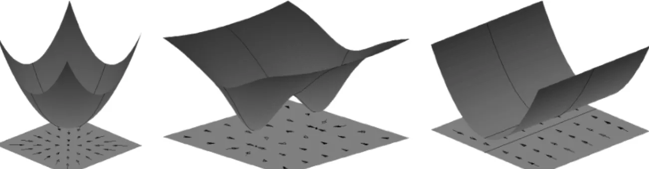
In the dynamical approach to ambiguity representation and resolution, the case of infinitely many solutions translates to the concept of continuous attractor dynamics. A unique solution to the inverse problem corresponds to a globally stable fixed-point attractor (see Fig. 2.8 (left)), where the point of attraction is parameterized by the input to the inverse model. Two solutions to the inverse problem relate to bi-stable attractor dynamics (see Fig. 2.8 (middle)). The input to the inverse model may drive the output feedback dynamics through a saddle node bifurcation: A single fixed-point attractor splits into two fixed-points separated by a saddle node (from Fig. 2.8 (left) to (middle)). These two fixed-points then manifest a two-valued solution set of the inverse model for a particular input. Continuous attractor dynamics model the limit case of infinitely many solutions by means of a continuous attractor manifold for a single input (see Fig. 2.8 (right)). Continuous attractor dynamics can be understood as an evenly leveled valley in the system’s associated energy function. Descending the energy landscape by iterating the dynamics yields a continuum of attractor states in the energy valley which are approached depending on the initial condition. In [56, 57], a model of continuous attractor dynamics is proposed to explain oculomotor control. I demonstrate continuous attractor manifolds of output feedback dynamics in Chapter 6 and Chapter 7.

In [29] and [58], a conceptually similar approach to represent the inverse kinematics of robotic manipulators by multi-stable terminal attractor dynamics has been proposed by Barhen, Gulati and Zak (sixth row in Tab. 2.1). However, it was not shown that their model is able to learn from ambiguous data or resolves ambiguities dynamically during operation. The network further does not model both, the forward and inverse model, and suffers from high computational load and bifurcations during learning. The implementation of output feedback dynamics to approximate multi-valued functions has been presented in [20]. However, the model also suffers from inefficient training and does not comprise a forward model.

The model proposed in this thesis learns the forward and inverse model efficiently and in a single network. The additional forward model is particularly useful in combination with feedback information from a plant: The network then implements a feedback control mechanism that estimates the current system state simultaneously to computing control commands. Moreover, integration of feedback from the plant renders control responsive to external perturbations. The proposed model resembles aspects of internal forward and inverse models that are also

(18)

Fig. 2.8: Energy landscape of output feedback dynamics. Convex energy landscape with a single fixed-point attractor (left): The same attractor is approached for all initial conditions. Energy landscape with two minima correspond to bi-stable dynamics (middle): One of two attractors is chosen depending on the initial condition. A saddle node exists in between both attractor basins. Energy landscape with a level valley exhibits continuous attractor dynamics (right): Depending on the initial condition, one of the infinitely many solutions (black line in the plane) is selected.

hypothesized to be implemented in the brain for motor control [13].

The dynamical approach to model ambiguous inverse problems crucially depends on the ability to shape multi-stable attractor dynamics that reflect the multiplicity of solutions. An efficient learning mechanism that enables shaping of attractor dynamics on demand is introduced in Chapter 4. The method from Chapter 4 is extended to a regularization framework which facilitates the robustness of training output feedback dynamics as is shown in Chapter 5. Several desirable properties of dynamical systems for inverse modeling will be provided in Chapter 7.

2.4

Flexible selection of models by associative completion

The associative paradigm to model forward and inverse relations can be further generalized to the flexible selection of mappings between the input and output spaces. To facilitate the further discussion, we concatenate data pairs to single vectors, i.e. u = (x,y). Associative completion means that a partially known patternuis completed by an (auto-)associative process [59, 60, 39]. For example, consider u _∈R3 with the first and the last component known only. Associative completion returns the second component:

  u1 × u3  _→   u1 u2 u3  

The core feature of associative completion is the flexible selection of the forward, inverse or a mixture of both models. That means any subset of components of u can be selected to query the model which then completes the complementary dimensions. Each constellation of inputs and outputs can be understood as a particular mapping, and there is apriori no preferred selection of inputs and outputs. However, incorporating the discussion above, it is important to distinguish the cases of unique and ambiguous mappings also in the context of associative completion. For instance, releasing an external input from the forward model can render the relation between selected inputs and outputs ambiguous. Note that associative completion differs from the approach to model each possible mapping between input and output space separately. Associative completion means that a single model is trained to represent the entire relation between input and output space. A particular model is then selected between parts of inputs and outputs during model exploitation.

Associative completion has been successfully implemented in non-dynamical associative models, for example by (parameterized) self-organizing maps using a flexible distance measure

(19)

Flexible selection of models by associative completion 13  u₂u(1k) u3    u₂(uk1+1) u3   h(u₁, u₂(k), u₃) z−1

Fig. 2.9: Associative completion implemented by output feedback dynamics: The hidden rep-resentation is externally driven by componentsu1 and u3. The complementary components, in

this case u2, are recalled dynamically by iterating the output feedback loop.

[59, 16, 39]. The dynamical implementation of associative completion is much less considered in the literature, although the basic concepts can be already found in [37] and [42]. Opposed to the recall of a stored pattern in traditional associative memories where the memory is retrieved from a completely determined initial condition, associative completion is an input-driven process. In case of dynamical associative memories, the processing units are clamped to, or driven by, the known part of the pattern throughout the recall process. Fig. 2.9 illustrates the implementation of associative completion by output feedback dynamics.

Seung proposes an associative completion mechanism that is implemented by an auto-encoder network ([27], seventh row in Tab. 2.1). A similar configuration is commonly applied in stacked auto-encoder models, where the feature representation of the input is concatenated with supervised pattern information, e.g. class labels, in the topmost layer. Label information is then recalled by a feedback process which is driven by the current input representation. A structurally similar process, i.e. probabilistic inference, is applied in Deep Belief Networks [61]. The dynamical or recurrent implementation of associative completion in case of static input data has not been explicitly discussed in the literature other than in [27], even though Jordan-type recurrent neural networks [15] comprise the same feedback feedback loop constellation and principally enable associative completion. This might be due to the typical application of Jordan (and Elman) networks to time-series prediction than to the association of static patterns [15, 25]. This thesis focuses on dynamical associative completion implemented in associative reser-voir computing (ARC, eighth row in Tab. 2.1) networks. The associative reservoir computing framework developed in Chapter 3 unifies a broad range of reservoir models and comprises output feedback dynamics with the modeling power outlined in Sec. 2.3.6. Output feedback dynamics moreover generalize the dynamical implementation of bidirectional mappings to as-sociative completion (compare Fig. 2.7 and Fig. 2.9). I show that output feedback dynamics of associative reservoir networks can be trained efficiently to model forward and inverse mappings including multiple solutions, associative completion and sequence transduction (Chapter 6 and Chapter 7). Finally, output feedback dynamics of associative reservoir networks are exploited for movement generation in feed-forward as well as feedback control systems (Chapter 8).

(20)

14 Asso ciativ e mo d el s, in v erse problems and am biguit y

Tab. 2.1: Taxonomy of associative models. The methods are related to each other with respect to their representation, dynamics, computational capabilities, and typical learning algorithms. Note that this is a rather broad overview and thus only some of the most prominent models for each conceptual niche are cited and described.

Method Representation Dynamics Computation Learning Citations Associative

Memory •distributed •none •auto- and hetero-association

•correlation-based •pseudo-inverse [38], [7], [37] BAM •distributed (•internal representation)

•attractor •bidirectional association •correlation-based [5], [4], [42],

[40], [41]

SOM

•local

•prototypes plus

topology

•none/winner takes all

(•lateral inhibition)

•dimension reduction •vector quantization

•discrete associative completion

•unsupervised vector quantization with topological constraint [62], [63], [39] PSOM •hybrid between

global and local

•prototypes plus

topology and basis functions

•winner takes all plus

continuous optimization

•forward and inverse mappings •continuous associative completion

•unsupervised vector quantization with topological constraint or supervised initialization [59], [60], [16] MMC •distributed •augmented variables

•attractor •ambiguous inverse mappings •none [49], [50],

[51]

Barhen

•distributed •internal

representation

•terminal attractor •ambiguous inverse mappings •generalization of

backpropagation [29], [58] Autoencoder with Associative Completion •distributed •internal representation •(continuous) attractor •variants with internal dynamics •auto-association

•continuous associative completion

•backpropagation •contrastive divergence •error correction [27], ([64], [65], [66]) Associative Reservoir Computing •distributed •internal representation •transients •(multi-stable) attractor •internal and output

feedback dynamics

•sequence transduction/generation •forward and (ambiguous)

inverse mappings

•continuous associative completion

•regression

•online least squares •intrinsic plasticity •state prediction

[22], [23], [67], [24], [55]

(21)

Chapter 3

Reservoir Computing with output

feedback

In this chapter, the basic idea of reservoir computing is introduced. Then, the associative reservoir computing model with output feedback is presented. Based on the associative reservoir computing framework, representative reservoir models are reviewed. The concepts of output feedback dynamics and stability are formalized.

3.1

The Reservoir Computing Paradigm

Learning in recurrent neural networks with hidden representations is typically implemented by gradient descent methods [68, 69]. Due to the recurrent network structure, optimizing the network parameters in closed form is not feasible in a direct way. Beside the enormous com-putational load of classical learning rules for recurrent networks, e.g. backpropagation through time, real time recurrent learning and Atiya-Parlos learning (see [68, 69] for an overview), bifur-cation of the network dynamics during iterative parameter adaptation do not allow guaranteed convergence to a local minimum of the error function.

In the recent decade, a different approach to training input-driven recurrent neural networks networks has been developed which considers the recurrent network as a fixed feature generating device that transforms the input signal into a spatio-temporal representation in the network state. This leads to the idea of separating a “harvesting” phase to record the states of the input-driven but otherwise fixed recurrent dynamics, and the output learning, which can be simple, linear, and efficient once the states are harvested. This approach has become popular when using a randomly initialized recurrent network as “rich reservoir of dynamics” [34].

Reservoir computing was introduced by Jaeger as Echo State Network (ESN, [30]) and independently by Maasset al. under the notion of Liquid State Machine (LSM, [70]). Learning of these reservoir networks is restricted to the weights that project the network state to special read-out neurons. Steil showed in [71] that this functional decomposition of a recurrent network into a fixed reservoir and an adaptive read-out layer arises naturally from the constrained optimization approach first introduced by Atiya and Parlos in [69]. Also, analyzing the weight dynamics during learning in recurrent neural networks shows a limited adaptation of the internal connections in relation to the read-out connections [72]. Restricting learning to the read-out weights circumvents bifurcations of the reservoir dynamics and the resulting problem of a moving target function that maps internal neuron activations to the desired outputs. Then, learning boils down to a simple linear regression problem and can be implemented very efficiently in an offline or online manner [30, 71]. Despite this restriction, the reservoir approach is still powerful because the strength of computing with a dynamical system is preserved: Transient network 15

(22)

16 Reservoir Computing with output feedback

states encode the history of external inputs and can serve as short-term memory.

The reservoir paradigm of using a non-linear dynamical system for computation has been implemented using various reservoir “substrates”. Typically, rate-coding or spiking neurons are utilized to build up a reservoir of dynamics [30, 70]. But also domain-specific reservoir models, e.g. comprising frequency sensitive neurons [73, 74, 75], can be used to build a reservoir. Recent research efforts try to exploit fast non-linear dynamics in photonic circuits for computation [76]. Fernando and Sojakka took the “liquid” approach literal and implemented a machine that can classify spoken digits using a bucket of water as reservoir substrate [77]. Even earlier than the formulation of echo state and liquid state approaches, the idea to use a fixed dynamical system instead of a fully trained recurrent neural network was proposed in [78] using iterative function systems as substrate of computation. These examples show that the general idea to read out the state of a dynamical system is very powerful. In the remainder of this thesis, however, only reservoirs comprising rate-coding neurons with sigmoidal activation functions are considered.

The reservoir computing paradigm to train only a perceptron-like read-out layer relies on the encoding of inputs in the reservoir by means of a “random, temporal and non-linear kernel” [79]. The mixture of both spatial and temporal components of the input is based upon three key ingredients: (i) the random projection into a high-dimensional state space (ii) with non-linearity introduced by typically sigmoidal activation functions and (iii) the recurrent connections in the reservoir implementing a short-term memory. On the one hand, the non-linear projection into a high-dimensional space is related to spatial kernel expansions which rely on the concept of a non-linear transformation of the original data into a high-dimensional space and the subsequent use of a simple, mostly linear, model. On the other hand, the recurrent connections implement a short-term memory by means of transient network states. Reservoir computing thereby exploits the “architectural bias“ [80] of recurrent neural networks with small weights to finite memory machines even prior to learning. Due to this short-term memory, reservoir networks are typi-cally utilized for temporal pattern processing such as time-series prediction, classification and generation [30]. In recent work, it is shown that recurrence in the reservoir also enhances the spatial encoding of static inputs in the reservoir [81]. Reservoir computing based on attractor states is therefore also suited for static pattern processing [82, 83, 84, 85].

3.2

Associative Reservoir Computing

In this thesis, a generalized version of reservoir networks is considered which extends the reser-voir computing paradigm to a bidirectional, associative setup. Associative Reserreser-voir Computing (ARC) is of particular interest in the context of sensory-motor tasks [22, 23]. A single network then learns the bidirectional relation between inputs and outputs: The mapping from sensory stimuli to motor commands, and the reverse mapping that can be used to predict or fill in missing sensory inputs. The network can either relate two (or more) time-series with each other, or be used in a static manner and learn to bidirectionally associate non-temporal signals. It further enables learning of ambiguous forward and inverse models [55], and implements an adaptive controller for movement generation [24, 55].

In the context of associative reservoir computing, feedback of the network output into the reservoir is a key ingredient. Although there are successful applications reported that use reservoir networks with output feedback [22, 23, 86, 71], the effects of output feedback have not been investigated systematically. In principle, I expect output feedback to add information of the output to the reservoir representation but also to cause additional transients which can be amplified in the worst case and result in a degraded performance. To grasp the problem of error amplification by output feedback, the concept of output feedback stability is introduced in this chapter. Alleviation of error amplification is a necessary prerequisite for robust association and this thesis mainly contributes to this question in Chapter 5 and Chapter 7.

(23)

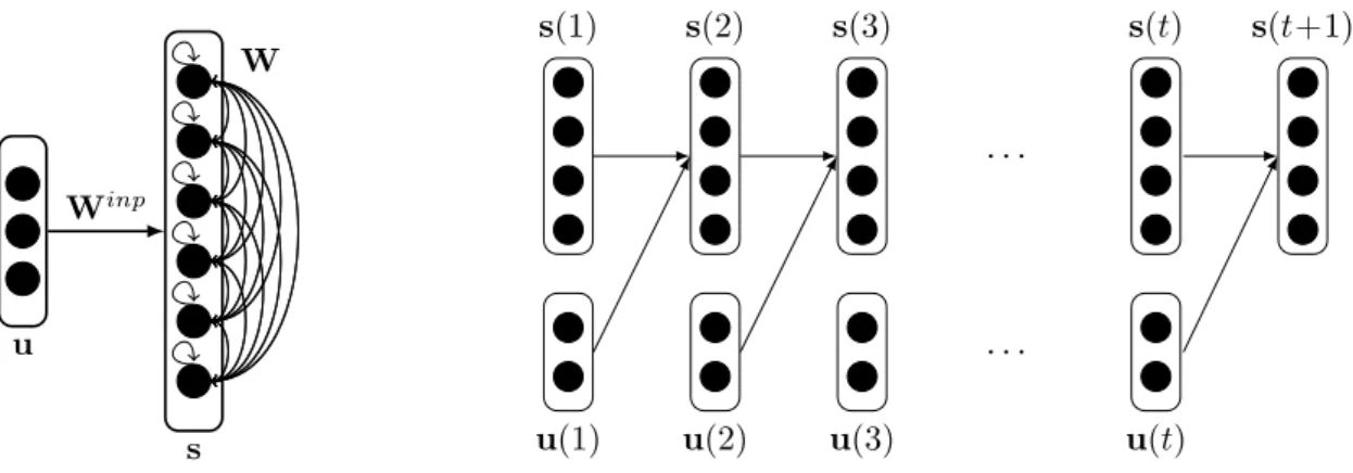
Associative Reservoir Computing 17 x y h 1 2 3 4 5 6 7 8 9 Wres Winp _Wout Wrec Wf db

Fig. 3.1: Associative Reservoir Computing setup: Inputs and outputs are bidirectionally con-nected via the internal representation in the reservoir.

reservoir neuronsh_∈RR_{that interconnect inputs}_x_∈_RD_{and outputs}_y_∈_RO_. _Wnet_captures

all connection sub-matrices between neurons in the network and is defined by

Wnet =       0 Wrec 0 Winp _Wres _Wf db 0 Wout 0      . (3.1)

Only connectionsWout_∈RO×RandWrec _∈RD×Rprojecting to the input and output neurons are trained by error correction (illustrated by dashed arrows in Fig. 3.1). All other weights, i.e. Winp ∈ RR×D_, _Wres _∈ _RR×R _and _Wf db _∈ _RR×O_{, are initialized randomly with small}

weights and remain fixed. Functionally, Winp, Wres and Wf db parameterize the excitation of the reservoir by inputs, outputs and the reservoir itself. The read-out weightsWout_{are trained}

to fit a desired input-to-output mapping from training examples, whereas Wrec is trained to reconstruct inputs from outputs.

Consider discrete reservoir dynamics

a(k+1) =Winpx(k) +Wresh(k) +Wf dby(k) (3.2)

h(k) =σ(a(k)) (3.3)

with time stepsk∈N, whereh(k) is obtained by applying non-linear activation functionsσi(·)

component-wise to the neural activationsai(k), i= 1. . . N. Typically, parameterized, sigmoidal

activation functions like the logistic function

hi=σi(ai) =

1

1 + exp (₋siai−bi)

(3.4) or the hyperbolic tangent

hi=tanhi(siai+bi) (3.5)

with slopessi and biasesbi are used. Input and output neurons have the identity as activation

function, i.e. are linear neurons, and are updated according to

y(k+1) =Wouth(k) (3.6)

(24)

The network dynamics can be compactly written by collecting input, reservoir, and output neurons in a vector z(k) = (x(k)T,h(k)T,y(k)T)T. Then, the dynamics of the entire system are described by

z(k+1) =σ(Wnetz(k)), (3.8) whereσ are then linear activation functions for input and output neurons.

3.2.1 Associative completion with output feedback dynamics

Association of inputs and outputs is accomplished by iterating output feedback dynamics. The forward model, which maps inputs to outputs, is queried by driving the network with external inputsx(k) while estimated outputs ˆy(k) are fed back into the hidden state in a recursive loop (compare Fig. 3.2). Equation (3.2) of the network dynamics changes to

a(k+1) =Winpx(k) +Wf dbyˆ(k) +Wresh(k). (3.9) Although the network’s input neurons are clamped to the external signal, an estimated value ˆ

x(k+1) =Wrech(x(k),yˆ(k)) =Wrecσ(Winpx(k) +Wf dbyˆ(k) +Wresh(k)) for these clamped neurons is also available. The forward model coins also the notion of output feedback dynamics because estimated outputs are fed back into the model.

For the backward model, which is externally driven by y(k), (3.2) alters to

a(k+1) =Winpxˆ(k) +Wf dby(k) +Wresh(k). (3.10) In this case, the estimated inputs are fed back recursively into the network, which is also referred to under the general notion of output feedback dynamics since then inputs become the functional outputs of the model.

Note that the forward path from inputsxto outputsy typically models an inverse problem in the sense of Chapter 2. This is often more convenient because generally applications require to solve inverse problems. With respect to this convention, the inverse model is “from left to right” (input-to-output) and the forward model “from right to left” (output-to-input).

x(k) ˆ y(k) ˆ x(k+1) ˆ y(k+1) h(k+1) 1 2 3 4 5 6 7 8 9 Wres z−1 Winp Wrec Wf db Wout input driving

Fig. 3.2: Output feedback dynamics of an associative reservoir network: Estimated outputs ˆy

from the last iteration step are fed back into the network whereas externally driven inputs are clamped to desired values x. Note that estimated outputs for externally driven inputs (here ˆx

(25)

Associative Reservoir Computing 19

The partial combination of both models is also possible which implements a mixed constraint satisfaction in input and output space. In a generic form, which also includes the cases of pure forward or backward mappings, the output feedback dynamics can be written as

a(k+1) =Winpˆx∗(k) +Wf dbyˆ∗(k) +Wresh(k) (3.11) with ˆx∗₍_k_{) = (ˆ}_x∗

1(k), . . . ,xˆ∗D(k))T, where ˆx∗i(k) = xi(k) for all constrained input components

i, and ˆx∗_i(k) = ˆxi(k) for all unconstrained input components. The same notational convention

applies to ˆy∗ and allows to flexibly mix constrained and unconstrained components in input and output space, i.e. associative completion.

3.2.2 Transient- and attractor-based computation

Originally, computation in reservoir networks is based on transient network dynamics and uti-lized for time-series processing where transient network states serve as short-term memory. Transients are temporally elusive but reproducible traces in the network state trajectory (see [87] for a discussion). In case of static, temporally non-contiguous data, transient dynamics by means of a short-term memory are not meaningful because each sample is independent of the previous one. Then, attractor-based computation, i.e. let the dynamics settle to a fixed-point attractor before the estimated output is interpreted, is favorable [82, 81].

Note that there are two distinguished “sources“ of dynamics considered in this thesis: (i) In-ternal dynamics of the reservoir layer set up by Wres_{, and (ii) dynamics due to the output}

feedback loop. Considering the reservoir dynamics, the mapping (x,y) 7→ ¯h from externally driven inputs to attractor statesh¯is unique if the reservoir subsystem is globally asymptotically stable. Unique attractor states of the reservoir layer are essential for learning of a functional relationship between inputs and outputs. Conditions for convergence of the reservoir layer are discussed more deeply in Sec. 3.2.3. Properties of the output feedback dynamics are the main topic of the following chapters. Depending on the task, globally stable, oscillatory or even multi-stable output feedback dynamics are targeted. Estimated outputs obtained from converged output feedback dynamics are denoted by ˆy(x). The same notation is utilized for estimated inputs ˆx(y).

In this section, technical details of monitoring the convergence of the network state are described. A short discussion of transient- and attractor-based computation in the context of different applications follows in Sec. 3.2.4.

Monitoring the convergence of reservoir networks

Application of the attractor-based computation scheme requires to monitor the convergence of the network state. The following algorithm monitors convergence of the state based on the fixed-point condition

h(k+1) =h(k). (3.12)

Algorithm 3.1 iterates the network dynamics (3.2), (3.3), (3.6) with clamped input pattern x

until the network state change ∆h falls below a small constant δ. The same scheme can be applied if the network is driven by outputs y or a combination of inputs and outputs. Algo-rithm 3.1 approximately terminates if the network state reaches a fixed-point, or the reservoir state does not converge inkmax iteration steps.

Algorithm 3.1 relies on the threshold δto determine convergence and is thus approximate in nature: If the network dynamics fulfill the fixed-point condition (3.12), convergence is identified correctly. But also state changes below the thresholdδ, which are not necessarily in the vicinity of a fixed-point, can be mistaken to be a fixed-point. However, Algorithm 3.1 has proven to be adequate if the admitted number of time stepskmax is sufficiently large andδ small.

(26)

Algorithm 3.1 Convergence algorithm

Require: get external inputx

Require: set k= 0, ∆h=_∞,δ= 10−6 _and _k

max= 1000

1: while∆h > δ andk < kmax do

2: inject external input xinto network 3: execute network iteration (3.2)–(3.7)

4: compute state change ∆h=kh(k)−h(k−1)k2

5: k=k+1

6: end while

7: returnk(if k=kmax, the network did not converge)

Observation of network convergence

The convergence criterion monitors whether an observable connected to the change of state in the network drops below a certain value. Measuring the state change directly as proposed in Algorithm 3.1 is rather inefficient. It is therefore useful to extend the framework to monitor the convergence of a network by considering different observables of the network state change. For example, measuring ∆h by _kh(k)₋h(k₋1)_k2 rather than_kh(k)₋h(k₋1)_k is an option which saves the computation of the square root. An adopted Hopfield energy of the network was utilized in [83] to monitor and verify convergence in experimental settings. These measures implement plainly the general idea of a change in state space of the network and are directly related to the common fixed-point condition (3.12). However, their computation is inefficient, either because the last network state has to be stored or the network weights are involved in their computation which results in quadratic complexity in the number of neurons.

A more efficient way of measuring the rate of change of the network state is to use the sum of its components, i.e. approximating ∆h by

k R X i=1 hi(k)− R X i=1 hi(k−1)k2.

This observable is ambiguous, i.e. there can be different states h(k) and h(k−1) while the component-wise sum of both states is equal. This case, however, is very rare. But, and this is important, the simplified observable of the state change is very efficient to compute and requires only the storage of a scalar from iteration k to k+ 1. In practice, the author could not observe any significant differences between using one of the above mentioned criteria and therefore applied the efficient implementation mostly in this thesis.

3.2.3 Network initialization and the Echo State Property

Supervised learning in the reservoir approach is restricted to weights Wrec and Wout that project the internal representation h to inputs and outputs. The remaining weight matrices

Winp, Wres and Wf db are randomly initialized and remain fixed. The initialization of these weights is therefore important for performance and stability [30, 88, 89]. Typically, the weights are drawn from an uniform distribution in [₋a?_{, a}?_{], where}_? _{denotes the respective sub-matrix}

W? of the network. Often, sparse connectivities 0≤ρ? ≤1 are preferred, whereρ? denotes the density of connections in the respective sub-matrix of the network.

More sophisticated initialization procedures for reservoir networks have been proposed that consider connectivity patterns according to topological constraints (see [90] for a discussion), or condensed reservoir creation schemes based on permutation matrices [91] and other reser-voir creation rules [92]. However, the gain in performance is rather restricted if initialization parameters are not adopted to the task at hand and therefore these specialized initializations

(27)

Associative Reservoir Computing 21

of the weight matrices are not further considered in this thesis. I stick to uniformly distributed network weights that are sometimes sparse but not according to a specific structure.

The reservoir matrix Wres _{plays a special role in the network configuration: The}

recur-rent reservoir connections introduce dynamics in the reservoir layer. These reservoir dynamics functionally serve as short-term memory [30] or, in case of attractor-based computation, non-linearly mix the input representation and produce complex features [89, 81]. In either case, it is important that these reservoir dynamics have some asymptotic properties, i.e. wash out initial conditions, such that the reservoir state is uniquely determined by a finite history of in-puts. This requirement for computation that reservoirs haveecho states has been formalized by Jaeger under the notion of the Echo State Property (ESP, [30]). The ESP implies global asymp-totic stability of the reservoir state in case of no output feedback connections (Wf db =0) [30]. Hence, reservoirs that have the ESP always converge to an unique attractor state for constant inputs independent of initial conditions. This is important for