Model-based programming environments for spreadsheets

(1)

Model-based Programming Environments for Spreadsheets

J´acome Cunhaa,c_{, Jorge Mendes}a,c_{, Jo˜ao Saraiva}a_{, Joost Visser}b a_{HASLab / INESC TEC, Universidade do Minho, Portugal}

b_{Software Improvement Group & Radboud University Nijmegen, The Netherlands} c_{CIICESI, ESTGF, Instituto Polit´ecnico do Porto, Portugal}

Abstract

Spreadsheets can be seen as a flexible programming environment. However, they lack some of the concepts of regular programming languages, such as structured data types. This can lead the user to edit the spreadsheet in a wrong way and perhaps cause corrupt or redundant data.

We devised a method for extraction of a relational model from a spreadsheet and the subsequent embedding of the model back into the spreadsheet to create a model-based spreadsheet programming environment. The extraction algorithm is specific for spreadsheets since it considers particularities such as layout and column arrangement. The extracted model is used to generate formulas and visual elements that are then embedded in the spreadsheet helping the user to edit data in a correct way.

We present preliminary experimental results from applying our approach to a sample of spreadsheets from the EUSES Spreadsheet Corpus.

Finally, we conduct the first systematic empirical study to assess the effectiveness and efficiency of this approach. A set of spreadsheet end users worked with two different model-based spreadsheets, and we present and analyze here the results achieved.

Keywords: Spreadsheets, Model-Driven Engineering, Model-Driven Spreadsheets, Empirical Validation

1. Introduction

Developments in programming languages are changing the way in which we construct programs: naive text edi-tors are now replaced by powerful programming language environments which are specialized for the programming language under consideration and which help the user throughout the editing process. Helpful features like highlight-ing keywords of the language or maintainhighlight-ing a beautified indentation of the program behighlight-ing edited are now provided by several text editors. Recent advances in programing languages extend such naive editors to powerful language-based environments [1, 2, 3, 4, 5, 6]. Language-based environments useknowledgeof the programming language to provide the users with more powerful mechanisms to develop their programs. This knowledge is based on thestructureand themeaningof the language. To be more precise, it is based on the syntactic and (static) semantic characteristics of the language. Having this knowledge about a language, the language-based environment is not only able to highlight keywords and beautify programs, but it can also detect features of the programs being edited that, for example, violate the properties of the underlying language. Furthermore, a language-based environment may also give information to the user about properties of the program under consideration. Consequently, language-based environments guide the user in writing correct and more reliable programs.

Spreadsheet systems can be viewed as programming environments for non-professional programmers, the so-calledend-userprogrammers . In order to improve end-user productivity, modern spreadsheet systems offer some of the mechanisms found in programming environments, as, for instance, auto completion of names/cells, or warnings when mismatching data types. These mechanisms, however, are very limited: they focus on thestructureof the data,

Email addresses:[email protected](J´acome Cunha),[email protected](Jorge Mendes), [email protected](Jo˜ao Saraiva),[email protected](Joost Visser)

(2)

and not on themeaningof the spreadsheet data. As a consequence, the end-user guidance provided by spreadsheets systems is very weak when compared to modern programming environments.

This paper extends previous work on generating powerful spreadsheet environment [7, 8]: we propose a technique to enhance a spreadsheet system with mechanisms to guide end users to introduce correct data. A background process adds formulas and visual objects to an existing spreadsheet, based on a relational database schema. To obtain this schema, or model, we follow the approach used in language-based environments: we use theknowledgeabout the data already existing in the spreadsheet to guide end users in introducing correct data. The knowledge about the spreadsheet under consideration is based on themeaning of its data that we infer using data mining and database normalization techniques.

Data mining techniques specific to spreadsheets are used to inferfunctional dependenciesfrom the spreadsheet data. These functional dependencies define how certain spreadsheet columns determine the values of other columns. Database normalization techniques, namely the use of normal forms [9], are used to eliminate redundant functional dependencies, and to define a relational database model. Knowing the relational database model induced by the spreadsheet data, we construct a new spreadsheet environment that not only contains the data of the original one, but that also includes advanced features which provide information to the end user about correct data that can be introduced. We consider several types of advanced features:auto-completion of column values,non-editable columns,

safe deletion of rows,key columnsandreference columns.

Besides presenting in this paper an extension of our previous work on generating spreadsheet programming envi-ronments, we also include in this paper both the first experimental results validating the proposed techniques, which are obtained by considering a large set of spreadsheets included in the EUSES Spreadsheet Corpus [10], and an em-pirical study evaluating the effectiveness and efficiency of the model-based spreadsheets. Both experiments show that our techniques work not only for database-like spreadsheets, like the example we will use throughout the paper, but they work also for realistic spreadsheets defined in other contexts (for example, inventory, grades or modeling).

This paper is organized as follows. Section 2 presents an example used throughout the paper. Section 3 presents our algorithm to infer functional dependencies and how to construct a relational model. Section 4 discusses how to embed assisted editing features into spreadsheets. A preliminary evaluation of our techniques is present in Section 5. In Section 6 we present an empirical validation of the spreadsheets we generate. Section 7 discusses related work and Section 8 concludes the paper.

2. Spreadsheet Programming Environments

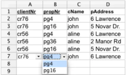
In order to present our approach we shall consider the following example taken from [11] and modeled in a spreadsheet as shown in Figure 1.

Figure 1: A spreadsheet representing a property rental system.

This spreadsheet contains information related to a housing rental system. It gathers information about clients, owners, properties, prices and rental periods. The name of each column gives a clear idea of the information it represents. We extend this example with three additional columns, nameddays (that computes the total number of rental days by subtracting the columnrentStart torentFinish),total (that multiplies the number of rental days by the rent per day value,rent) andcountry (that represents the property’s country). As usually in spreadsheets, the columnsdaysandrentare expressed by formulas.

This spreadsheet defines a valid model to represent the information of the rental system. However, it contains redundant information: the displayed data specifies the house rental of two clients (and owners) only, but their names are included five times, for example. This kind of redundancy makes the maintenance and update of the spreadsheet

(3)

complex and error-prone. A mistake is easily made, for example, by mistyping a name, thus corrupting the data on the spreadsheet.

Two common problems occur as a consequence of redundant data:update anomaliesanddeletion anomalies[12]. The former problem occurs when we change information in one place but leave the same information unchanged in the other places. The problem also occurs if the update is not performed exactly in the same way. In our example, this happens if we change the rent of property numberpg4from50to60only in one row and leave the others unchanged, for example. The latter problem occurs when we delete some data and lose other information as a side effect. For example, if we delete row 5 in the our example all the information concerning propertypg36is lost.

The database community has developed techniques, such as data normalization, to eliminate such redundancy and improve data integrity [12, 13]. Database normalization is based on the detection and exploitation of functional dependencies inherent in the data [14]. Can we leverage these database techniques for spreadsheets systems so that the system eliminates the update and deletion anomalies by guiding the end user to introduce correct data? Based on the data contained in our example spreadsheet, we would like to discover the following functional dependencies which represent the five entities involved in our house rental system:countries,clients,owners,properties, andrents

themselves:

country *∅ clientNr *cName ownerNr*oName

propNr *pAddress,rent,ownerNr

country,clientNr,propNr,rentStart,rentFinish*days,total

A functional dependencyA * Bmeans that if we have two equal inhabitants ofA, then the corresponding inhabitants ofB are also equal. For instance, the client number functionally determines his/her name, since no two clients have the same number. The right hand side of a functional dependency can be an empty set. This occurs, for example, in thecountryfunctional dependency. Although these are extreme cases for functional dependencies, they are formally valid [15]. To better explain their existence, let us consider a table in a database with a single attributecountry. To follow the guidelines of well-designed databases, this attribute would probably be primary key. The only functional dependency that holds in such a table iscountry *∅. This means that all the values in this table must be unique. In fact, as we will see in a few paragraphs, these cases will result in relational database tables where all the attributes are key, that is, all the entries in the table are unique.

Using these functional dependencies it is possible to construct a relational database schema. Each functional dependency is translated into a table where the attributes are the ones participating in the functional dependency and the primary key is the left hand side of the functional dependency. In some cases, foreign keys can be inferred from the schema. A foreign key (FK) is a set of attributes within one relation that matches the primary key of some relation. The relational database schema can be normalized in order to eliminate data redundancy. A possible normalized relational database schema created for the house rental spreadsheet is presented below.

country

clientNr,cName ownerNr,oName

propNr,pAddress,rent,#ownerNr

#country,#clientNr,#propNr,rentStart,rentFinish,days,total

This database schema defines a table for each of the entities described before. Note that the attributes marked with the symbol # areforeign keysto other tables and underlined attributes represent the key of the table. We explore this in Section 3. As we said, the first and the last tables are formed only by key attributes because the dependencies used to create them had no right-hand side.

In the next two sub-sections we will use all this information to create two different spreadsheets. The first one, termedschema-aware, is intended to keep the same structure as the original, but still with some features to guide users inputting correct data. The second one, namedrefactored, will have a different structure from the original one, since repeated information is removed and “entities” are factored out.

(4)

2.1. Schema-aware Spreadsheet Environment

Having defined a relational database schema we would like to construct a spreadsheet environment that respects that relational model, as shown in Figure 2, without changing the initial layout of the spreadsheet. This spreadsheet is from now on termedschema-aware.

Figure 2: A spreadsheet with auto-completion based on relational tables.

For example, this spreadsheet would not allow the user to introduce two different properties with the same property numberpropNr. Instead, we would like that the spreadsheet offers to the user a list of possible properties, such that he/she can choose the value to fill in the cell. Figure 3 shows a possible spreadsheet environment where possible properties can be chosen from acombo box.

Figure 3: Selecting possible values of columns using a combo box.

Using the relational database schema we would like to have a spreadsheet system offering the following features:

Auto-completion of Column Values. The columns corresponding to primary keys in the relational model determine the values of other columns; we want the spreadsheet environment to be able to automatically fill those columns provided the end user defines the value of the primary key.

For example, the value of the property number (propNr, columnB) determines the values of the address (pAddress, columnD), rent per day (rent, columnI), and owner number (ownerNr, columnK). Consequently, the spreadsheet environment should be able to automatically fill in the values of the columnsD,IandK, given the value of column B. SinceownerNr(columnK) is a primary key of another table, transitively the value ofoName(columnL) is also defined. This auto-completion mechanism has been implemented and is presented in the spreadsheet environment of Figure 2.

Non-Editable Columns. Columns that are part of a table (as the ones previously computed from the functional de-pendencies), but not part of its primary key must not be edited without some control. For example, columnLis part of the owner table but it is not part of its primary key. Thus, it must be protected from being edited arbitrarily. As we saw in the previous feature, they are edit through auto-completion, being this the only way to change their values.

The primary key of a table must not be randomly edited either since it can destroy the dependency. This feature prevents the end user from introducing potentially incorrect data and, thus, producing update anomalies. Still, such columns can be edited using the available combo boxes, as introduced before. Figure 4 illustrates this edit restriction.

Safe Deletion of Rows. Another usual problem with non-normalized data is the deletion problem. Suppose in our running example that row 5 is deleted. In such a scenario, all the information about the pg36 property is lost. However, it is likely that the user wanted to delete the rental transaction represented by that row only. In order to

(5)

Figure 4: In order to prevent update anomalies some columns must not be editable.

prevent this type of deletion problems, we have added a button per spreadsheet row (see Figure 2). When pressed, this button detects whether the end user is deleting important information included in the corresponding row. In case important information is removed by such deletion, a warning window is displayed, as shown in Figure 5.

Figure 5: Window to warn the end user that crucial information may be deleted.

Apart from these new features, the user can still access traditional editing features, and can rely on recalculation of functional dependencies in the background.

Traditional Editing. Advanced programming language environments provide both advanced editing mechanisms and traditional ones (i.e., text editing). In a similar way, a spreadsheet environment should allow the user to perform traditional spreadsheet editing, too. In traditional editing the end user is able to introduce data that may violate the relational database model that the spreadsheet data induces.

Recalculation of the Relational Database Model. Because standard editing allows the end user to introduce data violating the underlying relational model, we would like that the spreadsheet environment may enable/disable the safety features described in this section. When safety features are disabled, the end user would be able to introduce data that (temporarily) violates the (previously) inferred relational model. However, when the end user returns to safe editing, then the spreadsheet should infer a new relational model that will be used in future (safe) interactions.

2.2. Refactored Spreadsheet Environment

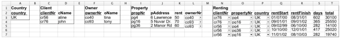
From the schema inferred we would also like to create a refactored spreadsheet which does not include any redundant information. Figure 6 presents such an optimized and modular spreadsheet for our running example. This spreadsheet is from now on termedrefactored.

Figure 6: The spreadsheet after applying the third normal form refactoring.

This new spreadsheet consists of five tables/modules, each one delimited by the empty column. In Figure 6, from left to right, we have a table forcountries, another forclients, forowners, forproperties, and for therenting

action itself. Note that all these tables are in a single worksheet for presentation purposes, only. In a real spreadsheet environment, however, they would be organized in different worksheets.

As we explained before, the obtained modularity solves three well-known problems in databases, namely the insertion, modification and deletion anomalies. These problems do not exist in the generated spreadsheet because data is normalized.

(6)

Key Columns. Moreover, we would like that the generated spreadsheet respected the schema. For example, in the

clientstable, the generated spreadsheet would not allow the user to introduce two clients with the same code, that is, the sameclientNr. If that error occurs, the spreadsheet system should warn the user as shown in Figure 7. Obviously, it is not possible to perform this validation in the original spreadsheet.

Figure 7: If the user introduces a new row in a table with a previously usedclientNrthe spreadsheet will immediately produce an error.

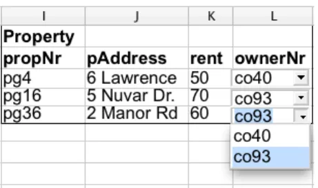
Reference Columns. The reader may have noticed that, for example, column L (Figure 6) containscombo boxeson the cells. From the relational schema, we can see that this column,ownerNr, is a foreign key to the owner code in theownerstable. In these cases, we would like that the new spreadsheet guarantees that the user only inserts values that already exist in the referenced table, since this is the definition of a foreign key. In fact, these columns should be locked for editing. This feature is illustrated in Figure 8.

Figure 8: Foreign key columns are filled in using combo boxes.

The refactored spreadsheet not only improves modularity and detects the introduction of incorrect data, but also eliminates redundancy: indeed, the redundancy present in the original spreadsheet has been eliminated. As expected, the names of the two clients occur only once.

In this section we have described an instance of our techniques. In fact, the spreadsheet programming environ-ments were automatically produced from the original spreadsheet displayed in Figure 1. In the following sections we will present in detail the techniques to perform such an automatic spreadsheet refactoring.

3. From Spreadsheets to Relational Databases

This section explains how to extract functional dependencies from the spreadsheet data and how to construct a normalized relational database schema modeling such data. These techniques were introduced in detail in our work on defining a bidirectional mapping between spreadsheets and relational databases [7]. In this section we present an extension to that algorithm that uses spreadsheet specific properties in order to infer a more realistic set of functional dependencies. Before we present the algorithm and our new extension, let us briefly introduce a few database definitions that are needed to understand functional dependencies.

Relational Databases. Arelational schemaRis a finite set of attributes{A1, ..., Ak}. Corresponding to each attribute

Aiis a setDi called thedomainofAi. These domains are arbitrary, non-empty sets, finite or countably infinite. A relation(ortable)ron a relation schemaRis a finite set oftuples(orrows) of the form{t1, ..., tk}. For eacht∈r,

t(Ai)must be inDi. Arelational database schemais a collection of relation schemas{R1, ..., Rn}. ARelational Database(RDB) is a collection of relations{r1, ..., rn}.

(7)

Each tuple is uniquely identified by a minimum non-empty set of attributes called aPrimary Key(PK). On certain occasions there may be more than one set suitable for becoming the primary key. They are designatedcandidate keys

and only one is chosen to become primary key. AForeign Key (FK) is a set of attributes within one relation that matches the primary key of some relation (possibly the same).

The normalization of a database is important to prevent data redundancy. Although there are several different normal forms, in general, a RDB is considered normalized if it respects theThird Normal Form(3NF) [11].

Discovering Functional Dependencies. In order to define the RDB schema, we first need to compute the functional dependencies presented in a given spreadsheet data. In [7] we reused the well known data mining algorithm, named FUN, to infer such dependencies. This algorithm was developed in the context of databases with the main goal of inferring all existing functional dependencies in the input data. As a result, FUNmay infer a large set of functional dependencies depending on the input data. For our example, we list the functional dependencies inferred from the data using FUN:

clientNr *cName,country

propNr *country,pAddress,rent,ownerNr,oName cName *clientNr,country

pAddress*propNr,country,rent,ownerNr,oName rent *propNr,country,pAddress,ownerNr,oName ownerNr *country,oName

oName *country,ownerNr

Note that, data contained in the spreadsheet exhibits all those dependencies. In fact, even the non-natural dependency rent *propNr,country,pAddress,ownerNr,oName is inferred. Indeed, the functional dependencies derived by the FUNalgorithm depend heavily on the quantity and quality of the data. Thus, for small samples of data, or data that exhibits too many or too few dependencies, the FUNalgorithm may not produce the desired functional dependencies. Note also that thecountry column occurs in most of the functional dependencies although only a single country actually appears in a column of the spreadsheet, namely UK. Such single value columns are common in spreadsheets. However, for the FUNalgorithm they induce redundant fields and redundant functional dependencies.

In order to derive more realistic functional dependencies for spreadsheets we have extended the FUNalgorithm so that it considers the following spreadsheet properties:

• Single value columns: these columns produce a single functional dependency with no right hand side (country*, for example). These columns are not considered when finding other functional dependencies.

• Semantic of labels: we consider label names as strings and we look for the occurrence of words likecode, number, nr, idgiven them more priority when considered as primary keys.

• Column arrangement: we give more priority to functional dependencies that respect the order of columns. For example,clientNr *cNamehas more priority thancName*clientNr.

Moreover, to minimize the number of functional dependencies we consider the smallest subset that includes all at-tributes/columns in the original set computed by FUN. The result of our spreadsheet functional dependency inference algorithm is:

propNr *pAddress,rent,ownerNr,oName

This set of dependencies is very similar to the one presented in the previous section. The exception is the last functional dependency which has an extra attribute (oName).

An important property to guarantee in a set of relational schemas is thelossless decompositionproperty.Lossless decompositionmeans that if we decompose a relation into smaller relations, it is possible to undo the process and recover the original relation.

(8)

Moreover, it is possible that some columns of our spreadsheet are not included in any functional dependency. To guarantee that they appear in the final schema and to ensure the lossless decomposition property we need to give an extra functional dependency to the algorithm. In fact, we use Maier’s strategy [15]: we generate an additional functional dependency which contains all the columns of our spreadsheet as antecedent (the exception are the ones defined by formulas). The consequent of the dependency is a newly introduced attribute, in this casenewAttribute, plus the attributes representing formulas (the relation between formulas and functional dependencies is explained in the following paragraphs). Note that this new attribute is just a “phantom” attribute required by the algorithm and can be removed when the final set of functional dependencies is created [15]. For our example such functional dependency is as follows:

country,clientNr,cName,ownerNr,oName,propNr,pAddress,rent,rentStart,rentFinish *days,total,newAttribute

Thus, the final set of functional dependencies is as follows:

propNr *pAddress,rent,ownerNr,oName

country,clientNr,cName,ownerNr,oName,propNr,pAddress,rent,rentStart,rentFinish *days,total,newAttribute

Spreadsheet Formulas. Spreadsheet systems differ from database systems by the use of formulas. Spreadsheet for-mulas define the values of some elements in terms of other elements. As a consequence, a formula explicitly defines a functional dependency. Such functional dependencies need to be included in the induced functional dependencies of our algorithm. Let us consider again the house rental spreadsheet, in which columndays is computed by sub-tracting the columnrentFinishfromrentStart: this is usually written as followsH3 = G3 - F3. This formula states that the values ofG3andF3determine the value ofH3, thus inducing the following functional dependency: rentStart, rentF inish * days.

Formulas can have references to other formulas. Consider, for example, the second formula of the running example J3 = H3 * I3, which defines the total rent by multiplying the total number of days by the value of the rent. BecauseH3is defined by another formula, the values that determine H3also determineJ3. As a result, the two formulas in our example induce the following functional dependencies:

rentStart,rentFinish *days rentStart,rentFinish,rent*total

In general, a spreadsheet formula of the following form X0 = f(X1, . . . , Xn) induces the following functional dependency: X1, . . . , Xn * X0. In spreadsheet systems, formulas are usually introduced by copying them through

all the elements in a column, thus making the functional dependency explicit in all the elements. This may not always be the case and some elements can be defined otherwise (e.g. by using a constant value or a different formula). In both cases, all the cells referenced must be used in the antecedent of the functional dependency.

These functional dependencies are useful for the mapping of spreadsheets to databases as presented in [7]. More-over, they are also used to create the final relational schema since they are necessary to construct the functional dependency that guarantees the lossless property.

Normalizing Functional Dependencies. Having computed the functional dependencies, we can now normalize them. Next, we show the results produced by thesynthesizealgorithm introduced by Maier in [15]. Thesynthesizealgorithm receives a set of functional dependencies as argument and returns a new set ofcompound functional dependencies. A

compound functional dependency(CFD) has the form(X1, . . . , Xn)* Y, whereX1, . . . , Xnare all distinct subsets

of a schemeR andY is also a subset ofR. A relation rsatisfies the CFD(X1, . . . , Xn) * Y if it satisfies the functional dependenciesXi * Xj andXi * Y, for all1 6 i,j 6 n. In a CFD,(X1, . . . , Xn)is theleft side,

(9)

applying this algorithm, all the functional dependencies with antecedents’ attributes representing formulas should be eliminated since a primary key must not change over time.

Next, we list the compound functional dependencies computed from the functional dependencies induced by our running example.

({country}) *∅

({clientNr}) *{cName} ({ownerNr})*{oName}

({propNr}) *{pAddress,rent,ownerNr}

({country,clientNr,propNr,rentStart,rentFinish})*{days,total,newAttribute}

Note that the redundant attributes have been removed. This derives directly from the normalization process introduced by Maier [15] where both redundant dependencies and redundant attributes are removed, that is, dependencies and attributes that do not add new information to the model are discarded. More details about this algorithm can be found in [15].

Computing the Relational Database Schema. Each compound functional dependency may define several candidate keys for each table. However, to fully characterize the relational database schema we need to choose the primary key from those candidates. To find such keys we use a simple algorithm: we produce all the possible tables using each candidate key as the primary key. In general, and since the set of functional dependencies is already reduced to its minimum, the sets of candidate keys are small (in many cases, as in the example, with only one element). Thus, not many combinations are generated. Finally, we apply again the same heuristics used to choose the functional dependencies to select the best tables from all the generated ones. For instance, we give more priority to tables that respect the order of columns than to others. The same happens to the other heuristics. In fact, we are just applying the same algorithm to choose the best functional dependencies to work with as before.

country

clientNr,cName ownerNr,oName

propNr,pAddress,rent,#ownerNr

#country,#clientNr,#propNr,rentStart,rentFinish days,total

This relational database model corresponds exactly to the one shown in Section 2. Note that the synthesize algorithm removed the redundant attributeoName that occurred in the last functional dependency through the normalization process. Note also that we have removed the “phantom” attribute (newAttribute) from the final model since it is no longer useful and is not part of the spreadsheet.

This set of functional dependencies completely characterizes our spreadsheet. Indeed to construct therefactored

spreadsheet all these dependencies are necessary. However, to construct the schema-aware spreadsheet, the last dependency is not necessary. Remember that it exists only to guarantee the lossless property, necessary when the data is rearrange and if one wants to have the data in its initial format later. Since in theschema-awarespreadsheet we do not rearrange the data, it is not necessary, and in fact, it would only duplicate some of the visual objects and formulas, not adding any new functionality.

More details about the system here presented to infer functional dependencies and compute a relational database schema from them can be found in [16].

4. Building Spreadsheet Programming Environments

This section presents techniques to refactor spreadsheets into powerful spreadsheet programming environments as described in Section 2. This spreadsheet refactoring is implemented as the embedding of the inferred functional dependencies and the computed relational model in the spreadsheet. This embedding is modeled in the spreadsheet itself by standard formulas and visual objects: formulas are added to the spreadsheet to guide end users to introduce correct data.

(10)

Before we present how this embedding is defined, let us first define a spreadsheet. A spreadsheet can be seen as a partial functionS :A→V mapping addresses to spreadsheet expressions. Elements ofSare calledcellsand are represented as(a, e). A cell address is taken from the setA =_N×_N. An expressione∈ Ecan be an input plain valuec∈Clike a string or a number, a reference to other cells using addressesa∈A, or a function namef ∈F that can be applied to one or more expressions:e∈E::=c|a|f(e, . . . , e).

4.1. Schema-aware Spreadsheet Environment

Let us start by defining the generation of the schema-aware spreadsheet. First, we show in detail how each computed relational table is used to provide an auto-completion mechanism in the spreadsheet environment. Next, we use the attributes of each relational table to include a non-editable mechanism on the programming environment, which will guide end users to avoid update inconsistencies. Next, we will show how to embed a mechanism that avoids the deletion of unintended data.

Auto-completion of Column Values. This feature is implemented by embedding each of the relational tables in the spreadsheet. It is implemented by a spreadsheet formula and a combo box visual object. The combo box displays the possible values of one column, associated to the primary key of the table, while the formula is used to fill in the values of the columns that the primary key determines.

Let us consider the tableownerNr,oName1from our running example. In the spreadsheet,ownerN ris in col-umnKandoN amein columnL. This table is embedded in the spreadsheet introducing a combo box containing the existing values in the columnK(as displayed in Figure 2). Knowing the value in the columnKwe can automatically introduce the value in columnL. To achieve this, we embed the following formula in row 7 of columnL:

S(L,7) =if(isna(vlookup(K7,K2:L6,2,0)),"",vlookup(K7,K2:L6,2,0))

This formula uses a (library) functionisnato test if there is a value in columnK. In case that value exists, it searches (with the functionvlookup) the corresponding value in the columnLand references it. The formulavlookupreceives the value to look for (or a reference to it), a range with two or more columns with data to be searched, the index of the column within the search range from where the result must be obtained, and a parameter that indicates whether the first column of the range is sorted in ascending order. If there is no selected value, it produces the empty string. The combination of the combo box and this formula guides the user to introduce correct data as illustrated in Figure 2.

We have just presented a particular case of the formula and visual object induced by a relational table. Next we present the general case. Letminrbe the very next row after the existing data in the spreadsheet,maxrthe last row

in the spreadsheet, andr1the first row with already existing data. Each relational database tablea1, ..., an, c1, ..., cm,

witha1, ..., an, c1, ..., cmcolumn indexes of the spreadsheet, induces firstly, a combo box defined as follows: ∀c ∈ {a1, ...,an},∀r ∈ {minr, ...,maxr}:

S(c,r) =combobox:={linked cell := (c,r);

source cells:= (c,r1) : (c,maxr)} secondly, a spreadsheet formula defined as:

∀c ∈ {c1, ...,cm},∀r ∈ {minr, ...,maxr}: S(c,r) =if (if (isna(vlookup((a1,r),(a1,r1) : (c,r−1),r−a1+ 1,0)), "", vlookup((a1,r),(a1,r1) : (c,r−1),r−a1+ 1,0)) == if (isna(vlookup((a2,r),(a2,r1) : (c,r−1),r−a2+ 1,0)), "", vlookup((a2,r),(a2,r1) : (c,r−1),r−a2+ 1,0)) == ...

(11)

== if (isna(vlookup((an,r),(an,r1) : (c,r−1),r−an+ 1,0)), "", vlookup((an,r),(an,r1) : (c,r−1),r−an+ 1,0)), vlookup((a1,r),(a1,r1) : (c,r−1),r−a1+ 1,0), "")

where==represents the mathematical equality test, which we have implemented as follows: a == b == c is defined in Excel asand(a =b,a=c). This formula must be used for each non primary key column created by our algorithm. Intuitively, this formula checks, for a given non primary key cell, if all the values chosen by the user from the primary key columns in the same row of that cell, agree on the value of the non primary key column. If so, then such a value is automatically inserted in the cell under consideration.

Let us consider the functional dependencycountry,ownerNr * propNr in our example. Note that this is a functional dependency that holds but is not used. Each cell of the columnpropNr receives an instance of the given formula. In this case the formula will have two innerif, one to checkcountryand another to checkownerNr. When in one row there are values chosen forcountryandownerNr, if thevlookupchecking these two columns finds the correspondingpropNrvalue to be the same, then such a value is shown in thepropNr cell.

In general, each conditionalif inside the mainif is responsible for checking a primary key column. In the case a primary key column value is chosen, soisna(vlookup (...))is true, the formula calculates the corresponding non primary key column value,vlookup(...). If the values chosen by all primary key columns are the same (represented by all the equality tests==), then that value is used in the non primary key column. This formula considers tables with primary keys consisting of multiple attributes (columns). Note also that the formula is defined in each column associated to non-key attribute values.

The example table analyzed before is an instance of this general one. In the tableownerNr,oName,ownerNris a1,oName isc1,cisL,r1is 2,minr is 7. The value ofmaxr is always the last row supported by the spreadsheet

system.

Foreign keys pointing to primary keys become very helpful in this setting. For example, if we have the relational tablesA, B andB, C whereB is a foreign key from the second table to the first one, then when we perform auto-completion in columnA, bothBandCare automatically filled in. This was the case presented in Figure 2.

Non-Editable Columns. To prevent wrong introduction of data, and thus, producing update anomalies, we protect some columns from random modification. Suppose in our example the user intends to insert a new entry registering the renting of propertypg36. If the system would let to insert again the property key, then by a mistake, the user could insert a different key for the same property, thus inputing inconsistent data. A similar situation could happen to non-key columns. Thus, a relational table, such asa1, ..., an, c1, ..., cm, induces the non-editability of columns

a1, ..., an, c1, ..., cmin an arbitrary way. That is to say that all columns that form a table become non-editable, unless

the user explores the system features. For non-key columns this means to use the auto-completion feature. That is, non-key columns are edited when key column change since the key value automatically fill in the non-key ones. On the other hand, key columns are edited when the user selects values from the existing combo boxes. Figure 4 illustrates such a restriction. In the case where the end user really needs to change the value of such protected columns, we provide traditional editing (explained below).

Safe Deletion of Rows. Another typical problem with non-normalized data is the deletion of data. Suppose in our running example that row 5 is deleted. All the information about propertypg36is lost, although the user would probably want to delete that rental transaction only. To correctly delete rows in the spreadsheet, a button is added to each row in the spreadsheet as follows: for each relational tablea1, ..., an, c1, ..., cmeach button checks, on its

corresponding row, the columns that are part of the primary key,a1, ..., an. For each primary key column, it verifies

whether the value to remove is the last one.

Letc∈ {a1, ..., an}, letrbe the row where the button is positioned,r1be the first row of columncwith data and rnbe the last row of columncwith data. The test is defined as follows:

(12)

If the value is the last one of its kind, the spreadsheet warns the user (showMessage) as can be seen in Figure 5. If the user presses theOKbutton, the spreadsheet will remove the row. In the other case,Cancel, no action will be performed. In the case the value is not the last one, the row will simply be removed,deleteRow(r).

More specifically,isLastverifies if the value in the cell passed as argument is the last one of its kind, that is, if in the same column there is no other value like it. For instance, suppose in our example row2is deleted. Then, the value cr76in cell A3 would be the last one of its kind since there is no other cell with the same value in that column. The functionshowMessagesimply shows the alert message to the user. Finally,deleteRowdeletes the row that it receives as argument. All these functions are implemented in OpenOffice Basic and their code is omitted since it would not improve the understandability of the work.

This mechanism will be triggered, for instance, if the user tries to delete row5of our running example, since in columnpropNr this row contains the last data about the house with codepg36.

Traditional Editing. Advanced programming language environments provide both advanced editing mechanisms and traditional ones (i.e., text editing). In a similar way, a spreadsheet environment should allow the user to perform traditional spreadsheet editing too. Thus, the environment should provide a mechanism to enable/disable the safety features described in this section. When safety features are disabled, the end user may introduce data that violates the (previously) inferred relational model. However, when the end user returns to safe editing, the spreadsheet infers a new relational model that will be used in future (safe) interactions.

4.2. The Refactored Spreadsheet Environment

In this section we explain how to generate therefactoredspreadsheet.

Key Columns. The keys of the functional dependencies are represented in the spreadsheet by being underlined. For instance, the column labeledclientNris underlined and this is the key of the client’s table. As in relational databases there cannot be two rows with the same key. If such a situation occurs, the spreadsheet will warn the user as shown in Figure 7.

The column immediately after each table contains a formula that computes whether there are two equal values in the key columns. For clients the formula is shown next:

=if (and($c$3 : $c$6501<>"";countif($c$3 : $c$6501; $c$3 : $c$6501)>1);"ERROR!";"")

Assuminga1is the reference to the first cell with data of the key column andanis the reference to the last, generically

this formula is constructed as follows:

=if (and(a1:an<>"";countif(a1:an;a1:an)>1;"ERROR!";"")

Theif condition calculates if there are repeated values. If so, the string"ERROR!"is shown, otherwise, the empty string populates the cell.

Reference Columns. The second feature thisrefactoredenvironment provides is safe references to other tables. In the relational database realm these are known asforeign keys. Since we have this information from the relational schema calculated before, we can integrate it in the spreadsheet. For instance, the table containing the properties has a reference to the property’s owner, in column L. As shown in Figure 8 such column containscombo boxesin the cells. Thus, these cells can only contain owners that in fact exist in the spreadsheet.

To accomplish this, each relational database table#am, ...,#an, an+1, ..., ar,#bs, ...,#bt, ..., bt+1, ..., bu that

references another tablecm, ..., cn, cs, ..., ct, d1, ..., dk, wherea∗, b∗, c∗, d∗ are column indexes of the spreadsheet,

induces a combo box defined as follows: ∀(ix) ∈ {am, ...,an} ∪ {bs, ...,bt}:

S(ix,r) =combobox:={linked cell:= (ix,r);

source cells:= (cx,minr) : (cx,maxr)}

whereminris the very first row with data in the spreadsheet,maxrthe last row in the spreadsheet. This means that

each column that is a reference to another column will have a combo box with the values available in the referenced column.

(13)

4.3. HaExcel Add-in

We have implemented the FUNalgorithm, the extensions described in this paper, thesynthesizealgorithm, and the embedding of the relational model in the HASKELLprogramming language [17]. We have also defined the mapping from spreadsheet to relational databases in the same framework named HaExcel [7]. Finally, we have extended this framework to produce the visual objects and formulas to model the relational tables in the spreadsheet. An Excel add-in has been also constructed so that end users can use spreadsheets in this popular system and at the same time our safety features.

5. Applicability Experiment

In this section we present an experiment performed to evaluate the applicability of our approach. Indeed we want to answer a single question: can this approach be applied to a wide range of spreadsheets? If this is not possible, then the approach needs more work. On the other hand, if this can be applied widely to spreadsheets, then we have a starting point.

For this we have run an experiment using the EUSES Corpus [10]. This corpus was conceived as a shared resource to support research on technologies for improving the dependability of spreadsheet programming. It contains more than 4500 spreadsheets gathered from different sources and developed for different domains. These spreadsheets are assigned to eleven different categories including financial (containing 19% of the total number of spreadsheets), inventory (17%), homework (14%), grades (15%), database (17%) and modeling (17%) (the remaining 1% represents other spreadsheets). Among the spreadsheets in the corpus, about 4.4% contain macros, about 2.3% contain charts, and about 56% do not have formulas being only used to store data. This corpus is widely accepted by the research community and has been used in other works [18, 19, 20].

In this experiment we have selected the first ten spreadsheets from each of the eleven categories of the corpus. We then applied our tool to each spreadsheet, obtaining different results (see also Table 1): a few spreadsheets failed to parse, due to glitches in the Excel to Gnumeric conversion (which we use to bring spreadsheets into a processable form). Other spreadsheets were parsed, but no tables could be recognized in them,i.e., their users did not adhere to any of the supported layout conventions. The layout conventions we support are the ones presented in the UCheck project [21], for instance, it is not possible to work with spreadsheets that have only sparse filled cells not forming a table or tables, neither with spreadsheets that do not label each table in the first row or column. This was the case for about half of the spreadsheets in our experiment. The other spreadsheets were parsed, tables were recognized, and edit assistance was generated for them. We will focus on the last groups in the upcoming sections.

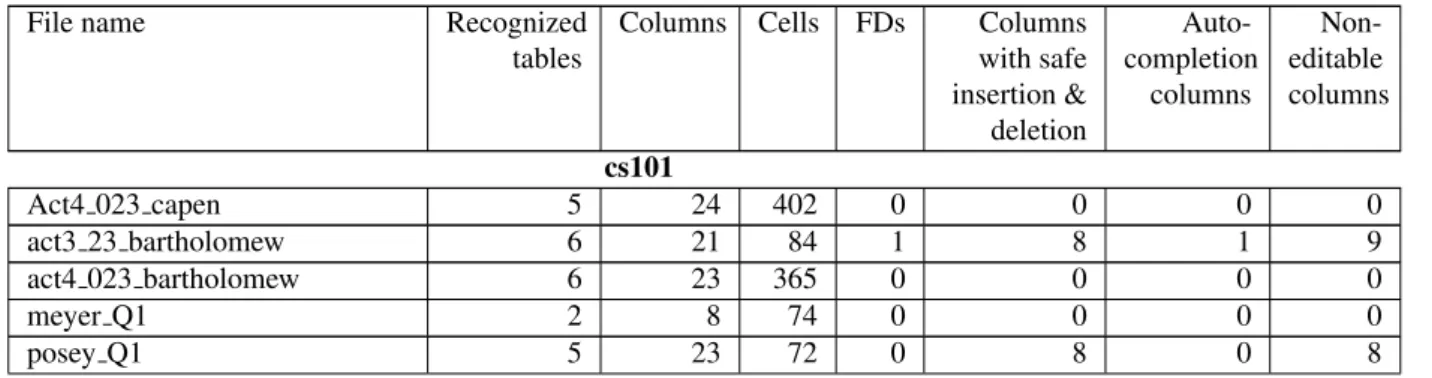
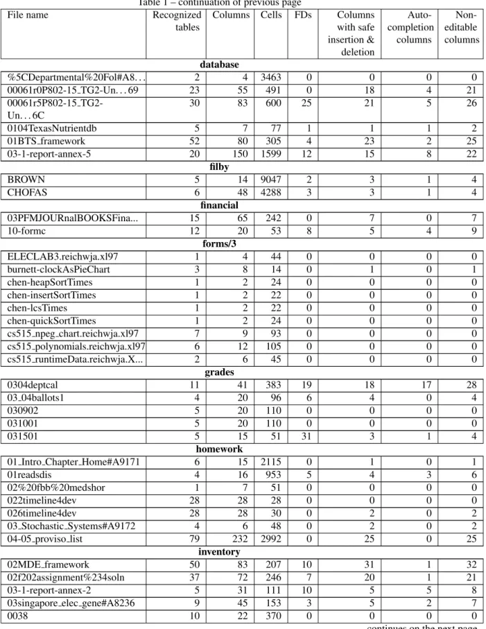
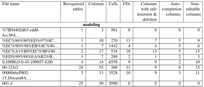
Processed Spreadsheets. The results of processing our sample of spreadsheets from the EUSES corpus are summa-rized in Table 1. The rows of the table are grouped by category as documented in the corpus. The first three columns contain size metrics on the spreadsheets. They indicate how many tables were recognized, how many columns are present in these tables, and how many cells. For example, the first spreadsheet in thefinancialcategory contains 15 tables with a total of 65 columns and 242 cells.

Table 1: Results of processing the selected spreadsheets.

File name Recognized

tables

Columns Cells FDs Columns

with safe insertion & deletion Auto-completion columns Non-editable columns cs101 Act4 023 capen 5 24 402 0 0 0 0 act3 23 bartholomew 6 21 84 1 8 1 9 act4 023 bartholomew 6 23 365 0 0 0 0 meyer Q1 2 8 74 0 0 0 0 posey Q1 5 23 72 0 8 0 8

(14)

Table 1 – continuation of previous page

tables

with safe insertion & deletion Auto-completion columns Non-editable columns database %5CDepartmental%20Fol#A8. . . 2 4 3463 0 0 0 0 00061r0P802-15 TG2-Un. . . 69 23 55 491 0 18 4 21 00061r5P802-15 TG2-Un. . . 6C 30 83 600 25 21 5 26 0104TexasNutrientdb 5 7 77 1 1 1 2 01BTS framework 52 80 305 4 23 2 25 03-1-report-annex-5 20 150 1599 12 15 8 22 filby BROWN 5 14 9047 2 3 1 4 CHOFAS 6 48 4288 3 3 1 4 financial 03PFMJOURnalBOOKSFina... 15 65 242 0 7 0 7 10-formc 12 20 53 8 5 4 9 forms/3 ELECLAB3.reichwja.xl97 1 4 44 0 0 0 0 burnett-clockAsPieChart 3 8 14 0 1 0 1 chen-heapSortTimes 1 2 24 0 0 0 0 chen-insertSortTimes 1 2 22 0 0 0 0 chen-lcsTimes 1 2 22 0 0 0 0 chen-quickSortTimes 1 2 24 0 0 0 0 cs515 npeg chart.reichwja.xl97 7 9 93 0 0 0 0 cs515 polynomials.reichwja.xl97 6 12 105 0 0 0 0 cs515 runtimeData.reichwja.X... 2 6 45 0 0 0 0 grades 0304deptcal 11 41 383 19 18 17 28 03 04ballots1 4 20 96 6 4 0 4 030902 5 20 110 0 0 0 0 031001 5 20 110 0 0 0 0 031501 5 15 51 31 3 1 4 homework

01 Intro Chapter Home#A9171 6 15 2115 0 1 0 1

01readsdis 4 16 953 5 4 3 6 02%20fbb%20medshor 1 7 51 0 0 0 0 022timeline4dev 28 28 28 0 0 0 0 026timeline4dev 28 28 30 0 2 0 2 03 Stochastic Systems#A9172 4 6 48 0 2 0 2 04-05 proviso list 79 232 2992 0 25 0 25 inventory 02MDE framework 50 83 207 10 31 1 32 02f202assignment%234soln 37 72 246 7 20 1 21 03-1-report-annex-2 5 31 111 10 5 5 8

03singapore elec gene#A8236 9 45 153 3 5 2 7

0038 10 22 370 0 0 0 0

(15)

Table 1 – continuation of previous page

tables

with safe insertion & deletion Auto-completion columns Non-editable columns modeling %7B94402d63-cdd8-4cc3#A. . . 1 3 561 0 0 0 0 %EC%86%90%ED%97%8C. . . 1 10 270 13 7 5 9 %EC%9D%98%EB%8C%80. . . 1 7 1442 4 4 5 6 %EC%A1%B0%EC%9B%90. . . 2 17 534 18 13 5 15 %ED%99%98%EA%B2%B. . . 3 7 289 2 1 2 3 0,10900,0-0-45-109057-0,00 4 14 6558 9 9 2 10 00-323r2 24 55 269 31 9 6 15 00000r6xP802-15 Docum#A. . . 3 13 3528 10 9 3 11 003 4 25 50 2090 0 0 0 0

The fourth column shows how many functional dependencies were extracted from the recognized tables. These are the non-trivial functional dependencies that remain after we use our extension to the FUNalgorithm to discard redundant dependencies. The last three columns are metrics on the generated edit assistance. In some cases, no edit assistance was generated, indicated by zeros in these columns. This situation occurs when no (non-trivial) functional dependencies are extracted from the recognized tables. In the other cases, the three columns respectively indicate:

• For how many columns a combo box has been generated forcontrolled insertion. The same columns are also enhanced with thesafe deletion of rowsfeature.

• For how many columns theauto-completion of column valueshas been activated,i.e., for how many columns the user is no longer required to insert values manually.

• How many columns are locked to prevent edit actions where information that does not appear elsewhere is deleted inadvertently.

For example, for the first spreadsheet of theinventorycategory, combo boxes have been generated for 31 columns, auto-completion has been activated for 1 column, and locking has been applied to 32 columns. Note that for the categoriesjacksonandpersonal, no results were obtained due to absent or unrecognized layout conventions or to the size of the spreadsheets (more than 150,000 cells).

Observations. On the basis of these results, a number of interesting observations can be made. For some categories, edit assistance is successfully added to almost all spreadsheets (e.g.inventoryanddatabase), while for others almost none of the spreadsheets lead to results (e.g. theforms/3category). The latter may be due to the small sizes of the spreadsheets in this category. For thefinancialcategory, we can observe that in only 2 out of 10 sample spreadsheets tables were recognized, but edit assistance was successfully generated for both of these.

Thepercentageof columns for which edit assistance was generated varies. The highest percentage was obtained for the second spreadsheet of themodelingcategory, with 9 out of 10 columns (90%). A good result is also obtained for the first spreadsheet of thegradescategory with 28 out of 41 columns (68.3%). On the other hand, the 5th of the

homeworkcategory gets edit assistance for only 2 out of 28 columns (7.1%). The number of columns with combo boxes often outnumbers the columns with auto-completion. This may be due to the fact that many of the functional dependencies are small, with many having only one column in the antecedent and none in consequent.

In summary, from 102 selected spreadsheets (although there are 11 categories,personalonly has 5 spreadsheets andcs101only 7) we could automatically process 50 spreadsheets. From these 50 spreadsheets, we could automati-cally generate assistance for 33 (66%). Thus, we could generate in an automatic fashion an environment for more than

(16)

32% of all spreadsheets from the 11 different categories. This percentage could be improved if our parsing system for spreadsheets was better. In fact, considering only the ones we could parse, our technique could create assistance for 66% of such spreadsheets.

Discussion. Our experiment justifies two conclusions. Firstly, the tool is able to successfully add edit assistance to a series of non-trivial spreadsheets. A more thorough study of these and other cases can now be done to identify techni-cal improvements that can be made to the algorithms for table recognition and functional dependency extraction. For instance, for the categoriesjacksonandpersonalwe could not use any spreadsheets, and thus these are spreadsheets that we can study to improve our algorithms. Secondly, in the enhanced spreadsheets a large number of columns are generally affected by the generated edit assistance, which indicates that the user experience can be impacted in a significant manner. Thus, a validation experiment can be started to evaluate how users experience the additional assistance and to which extent their productivity and effectiveness can be improved. In fact we present in the next section such a study.

As a final remark we note that it is not possible to make any judgment about the quality of the generated environ-ments. This would require another study, with real users and their spreadsheets. After applying our techniques to their spreadsheets users would need to evaluate the results, based on the benefits of such results. This would also require to train such users to work with these new spreadsheets. Unfortunately, such a study is outside of the scope of this paper. Nevertheless, in another study presented in [22] we have used the same technique here presented to infer functional dependencies from spreadsheets and used them to automatically create models to those spreadsheets. In that work we have shown that more than 76% of all models generated aregoodmodels (in a scale with the gradesbad,acceptable, andgood). Although this cannot be used to prove that the environments we here generate are of the same quality, since we are using the same technique to infer the structure and the functional dependencies that are the same for both works, we believe this gives a good hint about the generated environments.

6. Empirical Validation

In this section, we present an empirical study that we have conducted with the aim of analyzing the influence of using models in end-user spreadsheet productivity. In this study we consider both model-based spreadsheets proposed in this paper. We will refer to the refactored spreadsheet asrefactoredand to the other asschema-aware, as apposed to anoriginalspreadsheet (without any model).

We assess end-user productivity in introducing, updating and querying data in those two model-based spreadsheets and in a traditional one. As the models we consider representative database-like spreadsheets. It should be clear that we are not analyzing all possible (types of) spreadsheets. Nevertheless, even considering spreadsheets strongly related to databases, the domain of our tests is clearly the spreadsheet environment.

In this paper we wish to answer the following research questions:

RQ1 Do end users introduce fewer errors when they use one of the model-based spreadsheets versus theoriginal

unmodified one?

RQ2 Does a particular model-based spreadsheet lead to fewer errors in particular tasks when compared to theoriginal

one?

RQ3 Are end users more efficient using the model-based spreadsheets than using theoriginalone?

6.1. Study Design

As suggested in [23] we have divided this study in five different phases. Next we briefly summarize each of them so the reader can better understand the remaining of this section.

1 - Formulating hypothesis to test. After several discussions and meetings we finally formulated the hypothesis pre-sented in this work: model-based spreadsheets can help end users committing less errors when editing and querying spreadsheets. More details in Section 6.1.4.

(17)

2- Observing a situation. Once we got enough and appropriate qualified participants we ran the study itself. In this case we selected 38 participants that were not studying any majors related to computer science or informatics (see Section 6.1.2). During the study, we screen casted the participants’ computers and afterwards we collected the spreadsheets they worked on.

3 - Abstracting observations into data. We computed a series of statistics, that we present in detail in Section 6.2, over the spreadsheets participants developed during the study: we graded their performance and measured the time they took to perform the proposed tasks. All the data we used is available at theSSaaPPproject web page http://ssaapp.di.uminho.pt. The tasks and the spreadsheets participants received are also available.

4 - Analyzing the data. The enormous collection of data that we gathered was later systematically analyzed. Each participant worked on three different spreadsheets and these three spreadsheets required the verification of 376 cells to assess the participant’s answers (this was done mostly automatically). This analysis is presented in more detail in Section 6.2.

5 - Drawing conclusions with respect to the tested hypothesis. Based on the results we obtained, we finally drew some conclusions. We were also able to suggest some future research paths based on our work, which are presented in the Section 6.4.

Our study aimed to answer whether participants were able to perform their tasks with more accuracy and/or faster given the experimental environments. We used a within-subjects design2_{, where each participant received 3}

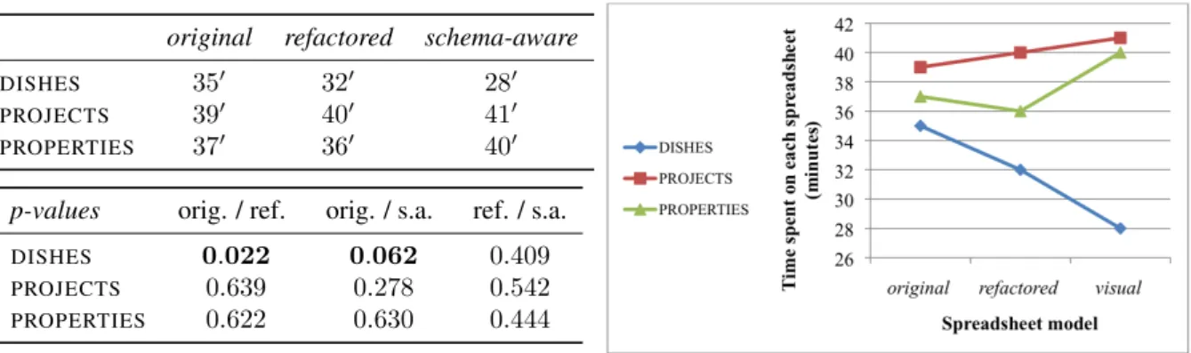
spreadsheets, one for each problem (DISHES, PROJECTS,PROPERTIES). Each of the 3 spreadsheets was randomly distributed under one of the 3 model (original,refactored,schema-aware). Participants were asked to do various tasks in each spreadsheet: data entry, editing, and calculations. They were encouraged to work as quickly as possible, but were not given time limits.

6.1.1. Methodology

Participants started the study by filling out a background questionnaire so we could collect their area of study and previous experience with spreadsheets, other programming languages and English comfort (Portuguese is their native language). An introduction to the study was given orally in English, this was explicitly not a tutorial for the different environments because the goal was to see if even without any introduction to the various models the participants would still be able to understand and complete the tasks. Since the order of the spreadsheets was randomized, they were told that the other sitting around them might appear to be moving faster, but that some tasks were shorter than others. After2hours participants were stopped if they were not already finished. Following the tasks they had a post session questionnaire which contained questions assessing their understanding of the different models, (3questions forrefactoredand4forschema-aware). Correct answers could only be given by participants having understood the running models. Grading the questionnaires was done as follows: a correct answer receives total points; an incorrect answer receives 0 points and an answer that is not incorrect nor (totally) correct receives half of the points. We recorded the users’ screens using screen capture technology. At the end of the study the user-completed spreadsheets were saved and graded for later analysis.

6.1.2. Participants

Recruitment was conducted through a general email message to the university, asking for students with spread-sheet experience and comfort with English. Of the hundreds that responded (there was a compensation involved), participants were selected based on spreadsheet experience, comfort with English, and majors outside of computer science and engineering. In total, 38 participants finished the study with data we were able to use (25 females, 11 males, and 2 who did not answer about their gender). Two participants did not try to solve one of the proposed tasks; for these participants, we included in the study only the tasks they undertook. A few participants’ machines crashed and therefore they were eliminated from the study. The majority of participants were between 20-29 years of age, with

2_{A within-subjects design means that all treatments (in our case, the three different models) were applied to all participants, as opposed to have}

each treatment applied to different set of participants (in our case this would have mean to have three different sets of participants, each of which using a different model).

(18)

the remaining under 20. All were students at the university. About 2/3 were working on their Bachelor’s degree, the remaining on their Masters. None were studying computer science or engineering and the most represented majors were medicine, economics, nursing and biology. A variety that is good for representing the end-user population of spreadsheets.

6.1.3. Tasks

The task lists were designed to include tasks that are known to be problematic in spreadsheets, which involve data insertion, edition and the use of formulas. The tasks were 1) add new information to the spreadsheet, 2) edit existing data in the spreadsheets and 3) do some calculations using the data in the spreadsheets.

Some of the tasks asked users to add many new rows of data, with the aim of a repetitive task being common in real-world situations. As we were designing the tasks, we imagined a type of data entry office scenario, where an office worker might receive on paper data which was initially filled out on a paper form and needed to be entered into a spreadsheet. This first task of data entry, in theory, should be fastest (and done with fewest entry errors) in the

refactoredspreadsheet. The second task, of making changes to existing data in a spreadsheet should also be easier within arefactoredspreadsheet, since the change only needs to be made in one location, and therefore there would be less chance of forgetting to change it. The final task was to do some calculations using the data in the spreadsheet, such as averages, etc. This task was added because of the frequency of problems with formulas.

One of the spreadsheets used in the study,PROPERTIES, stores information about a house renting system (adapted from [11]). This spreadsheet has information about renters, houses and their owners as well as the dates and prices of the rents.

A second spreadsheet,DISHES, contains information about sales of detergents to dish washers. Information about the detergents, prices and the stores where they are sold is present on this spreadsheets (adapted from [24]).

The last spreadsheet,PROJECTS, stores information about projects, like the manager and delivery date, employees, and the instruments used buy them (adapted from [25]).

In the task list forDISHES,67%(39out of58cells needed to be changed) of the tasks consist of inserting new data,21%(12/58) are editing tasks and12%(7/58) involve calculations over the data in the spreadsheet. In the task list forPROJECTS,80%(221/277) of the tasks are for inserting new data,7%(20/277) for edition and13%(36/227) for calculations. Finally, forPROPERTIES, inserting data tasks are56%(64/115) of the total, whereas data editing and calculation tasks are19%(22/115) and25%(29/115) of the total, respectively.

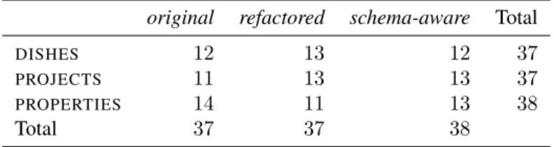
Grading the participants’ performance was done as follows. For tasks involving adding new data to the spreadsheet or performing calculations over spreadsheet data, whenever a participant executes a task as we asked him/her to, he/she is awarded100%of the total score for that task; on the contrary, if the participant does not at all try to solve a particular task, he/she gets no credit for that. An intermediate situation occurs when participants try to solve a task, but fail to successfully conclude it in its entirety. In this case, the participant is awarded50%of the score for that task. For tasks involving editing data, a value in the interval0%−100%is awarded according to the participants’ success rate in such tasks. Table 2 shows the number of participants that worked on each spreadsheet and each model. Note that the distribution of models and spreadsheets by the participants is homogeneous.

Table 2: Participants per spreadsheet/model.

original refactored schema-aware Total

DISHES 12 13 12 37

PROJECTS 11 13 13 37

PROPERTIES 14 11 13 38

Total 37 37 38

6.1.4. Hypotheses

In order to have an idea on how much relevant are the results obtained, we performed a statistical analysis. For that, we defined three kinds of hypotheses to test, one for each research question. Then, we tested each of this hypotheses with all combinations of models:originalvs.refactored(represented byorig. / ref.in the tables),original

(19)

vs. schema-aware(represented byorig. / s.a. in the tables), andrefactoredvs. schema-aware(represented byref. / s.a.in the tables). The hypotheses are formulated as follows:

• The null hypothesis forRQ1, HRQ10, is: the rate of correct tasks is equal between the two models tested.

HRQ10 : µx = µy, whereµxis the expected mean for the first model and µy is the expected mean for the

second model.

The alternate hypothesis,H1, is that the rate of correct tasks is different between the two models tested,HRQ11 :

µx6=µy.

This hypothesis is tested on each spreadsheet (i.e.,DISHES,PROJECTS, andPROPERTIES).

• The null hypothesis forRQ2, HRQ20, is: the rate of correct tasks is equal between the two models tested.

HRQ20 : µx = µy, whereµxis the expected mean for the first model and µy is the expected mean for the

second model.

The alternate hypothesis,H1, is that the rate of correct tasks is different between the two models tested,HRQ21 :

µx6=µy.

This hypothesis is tested for each task (i.e.,data insertion,data edition, andstatistics) on each spreadsheet (i.e., DISHES,PROJECTS, andPROPERTIES).

• The null hypothesis forRQ3,HRQ30, is: the time to perform the tasks is equal between the two models tested.

HRQ30 :µx =µy, whereµxis the expected mean time for the first model andµy is the expected mean time

for the second model.

The alternate hypothesis,H3, is that the time to perform the tasks is different between the two models tested, HRQ13 :µx6=µy.

This hypothesis is tested on each spreadsheet (i.e.,DISHES,PROJECTS, andPROPERTIES).

6.2. Analyzing End-User Performance

We divide the presentation of our empiric results under two main axes: effectiveness and efficiency. In studying effectiveness we want to compare the three running models for the percentage of correct tasks that participants pro-duced in each one. In studying efficiency we wish to compare the time that participants took to execute their assigned tasks in each of the different models. We start by effectiveness.

6.2.1. Effectiveness

Each participant was handed3different lists of tasks (insert, edit and query data) to perform on3different spread-sheets (DISHES,PROJECTS,PROPERTIES). Each spreadsheet, for the same participant, was constructed under a dif-ferent model (original,refactored schema-aware).

For each spreadsheet, and for each model, we started by analyzing the average of the scores obtained by partic-ipants. Moreover, we tested the hypothesesHE at the 0.05 significance level. The results of both the averages and

p-values from the hypothesis testing are displayed in Figure 9.

We notice that no spreadsheet model is the best for all spreadsheets in terms of effectiveness. Indeed, we may even notice that spreadsheets in the traditional style, theoriginalmodel, turned out to be the best for both theDISHES andPROPERTIESspreadsheets. Theschema-awaremodel suited the best for thePROJECTSspreadsheet. However, no significant statistical differences were found, except between the effectiveness of theoriginalmodel and the schema-awareone for theDISHESspreadsheet.

In the same line of reasoning, there is no worst model: refactored achieved the worst results forDISHES and PROJECTS;schema-awaregot the lowest average scores forPROPERTIES. Nevertheless, these results seem to indicate that the models that we have developed are not effective in reducing the number of errors in spreadsheets, since one of them is always the model getting the lowest scores. This first intuition, however, deserves further investigation. For one, on the theoretical side, one may argue thatoriginalis, without a doubt, themodelthat end users are accustomed to. Recall that in the study, we opted to leave out participants with computer science backgrounds, who could be more sensible to the more complex modelsrefactoredandschema-aware, preferring to investigate such models on traditional users of spreadsheets. On the other hand, we remark that these more complex models were not introduced; a part of our study was also to learn whether or not they could live on their own.

(20)

original refactored schema-aware

DISHES 86% 76% 78%

PROJECTS 73% 68% 78%

PROPERTIES 75% 64% 62%

p-values orig. / ref. orig. / s.a. ref. / s.a.

DISHES 0.184 0.0293 0.838

PROJECTS 0.344 0.5622 0.111

PROPERTIES 0.287 0.2625 0.833

Figure 9: The p-values obtained from testing the hypotheses at theHE0.05 significance level, and the average of the effectiveness scores obtained

by participants for each spreadsheet and for each model.

Our next step was to investigate whether the (apparent) poor results obtained by complex models are due to their own nature or if they result from participants not having understood them. So, we studied participations that did not achieve at least50%, which are distributed by the spreadsheet models as follows:original,0%,refactored,25%and

schema-aware,21%.

While inoriginalno participation was graded under50%, this was not the case forrefactoredandschema-aware, which may have degraded their overall average results. For these participations, we analyzed the questionnaire that participants were asked to fill in after the session. The average classifications for the post session questionnaires, for participations in the study that were graded under50%is24%forrefactoredand31%forschema-aware.

These results show that participants obtaining poor gradings on their effectiveness, also got poor gradings for their answers to the questions assessing how they understood the models they had worked with. In fact, such participants were not able to answer correctly (to at least) two thirds of the questions raised in the post session questionnaire. From such results we can read that1/4of participants was not able to understand the more complex models, which might have caused a degradation of the global effectiveness results for these models. This also suggests that if these models are to be used within an organization, it is necessary to take some time to introduce them to end users in order to achieve maximum effectiveness. Nevertheless, even without this introduction, the results show that the models are competitive in terms of effectiveness: at most they are13%worse than the originalmodel, and for one of the spreadsheets, theschema-awaremodel even got the best global effectiveness.

6.2.2. Effectiveness by Task Type

Next, we wanted to realize how effective models are to perform each of the different types of tasks that we have proposed to participants:data insertion,data editingandstatistics.

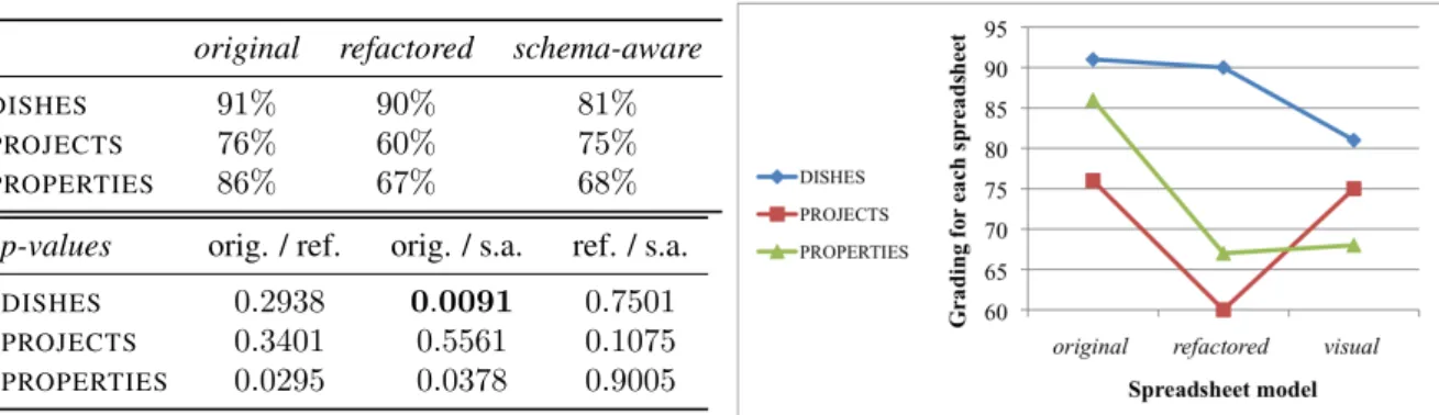
i)Data insertion: The results presented in Figure 10 show, for each model, how effective participants were in adding new information to the spreadsheets they received. The results of hypothesis testing are also present, namely the p-values.

Theoriginalmodel revealed to be the most effective, for all three spreadsheets, being closely followed by refac-toredandschema-awareforDISHES, and byschema-awareforPROJECTS. Therefactoredmodel, forPROJECTS, and the modelsrefactored andschema-aware, forPROPERTIES, proved not to be competitive for data insertion, in the context of the study. The differences that we obtained are not statistically significant, except when comparingoriginal

withschema-awarefor DISHES. Again, we believe that this in part due to these models not having been introduced previously to the study: the insertion of new data is the task that is most likely to benefit from totally understanding of the running model, and also the one that can be otherwise most affected. This is confirmed by the effectiveness results observed for other task types, that we present next.

ii) Data editing: Now, we analyze the effectiveness of the models for editing spreadsheet data. The results presented in Figure 11 show that once a spreadsheet is populated, we can effectively use the models to edit its data.

(21)

DISHES 91% 90% 81%

DISHES 0.2938 0.0091 0.7501

PROJECTS 0.3401 0.5561 0.1075 PROPERTIES 0.0295 0.0378 0.9005

Figure 10: Effectiveness results for data insertion.

DISHES 91% 82% 82%

DISHES 0.202 0.455 0.622

PROJECTS 0.440 0.996 0.381

PROPERTIES 0.008 0.322 0.002

Figure 11: Effectiveness results for data edition.

This is the case ofrefactoredforPROJECTSand specially forPROPERTIESwhere there is statistical significance in the differences comparing to the other two models.Originalis the most effective in data editing forDISHES. Schema-awareis comparable torefactoredfor DISHES, but for all other spreadsheets, it always achieves the lowest scores among the three models.

iii)Statistics:Finally, we have measured the effectiveness of the models for performing calculations over spread-sheet data, obtaining the results shown in Figure 12.

DISHES 52% 37% 57%

DISHES 0.197 0.653 0.119

PROJECTS 0.289 0.372 0.878

PROPERTIES 0.375 0.676 0.687

Figure 12: Effectiveness results for statistical calculations.

We can see thatschema-awareobtained the best results forDISHES, and thatrefactoredobtained the best results for both spreadsheetsPROJECTSandPROPERTIES. We can also see that theoriginalmodel was the worst model for