Modeling the Dependence Structure of the WIG20 Portfolio Using a Pair-copula Construction

Full text

(1)DYNAMIC ECONOMETRIC MODELS. ou. se. Vol. 10 – Nicolaus Copernicus University – Toruń – 2010. gH. Ryszard Doman. Pu b. lis. hin. Adam Mickiewicz University in Poznań. Sc. ien. tif. ic. Modeling the Dependence Structure of the WIG20 Portfolio Using a Pair-copula Construction†. icu sU. niv er. sit y. A b s t r a c t. Elliptical distributions commonly applied to modeling the returns of stocks in highdimensional portfolio are not capable of adequate describing the dependence between the components when their statistical properties are very diverse. The MGARCH and standard dynamic copula models are often of little usefulness in such cases. In this paper, we apply a methodology called the pair-copula decomposition to model the joint conditional distribution of the returns on stocks constituting the WIG20 index, and show some advantage of this construction over the approach using the t Student DCC model.. op er n. K e y w o r d s: dependence, portfolio, copula, pair-copula construction.. sC. 1. Introduction. ©. Co py. rig ht. by. Th. eN. ico lau. Elliptical distributions commonly applied to modeling the returns of stocks in high-dimensional portfolio are not capable of adequate describing the dependence between the components of the return vector when their statistical properties are very diverse. Except of a huge number of parameters necessary to estimate, this is why multidimensional GARCH models are often of little practical usefulness in such cases. Also the standard dynamic copula models which are successfully applied in the bivariate case are not so useful for large dimension because of a small number of classical multivariate copulas that are flexible enough to fit the data. In this context, a new approach to modeling multivariate data which exhibit complex patterns, proposed recently by Aas et al. (2009), has triggered off much interest. It was inspired by the work of Joe (1996), Bedford and Cooke (2002), and Kurowicka and Cooke (2006). The main idea of this methodology is to model dependence by decomposing higher-dimensional copula densities into bivariate ones (pair-copula densities) arising from the condi†. This work was financed from the Polish science budget resources in the years 2007-2010 as the research project NN 111 1256 33..

(2) Ryszard Doman. 32. Pu b. lis. hin. gH. ou. se. tional and unconditional distribution functions of the modeled variables. A further simplification of the decomposition can be then obtained basing on conditional independence. In this paper, we apply the pair-copula decomposition approach to model the joint conditional distribution of the returns on stocks constituting the WIG20 index. Results of our investigation support a view that this construction not only is superior over the approach that uses multidimensional t copula model but also represents a promising technique of building flexible and accessible multivariate extensions of classical bivariate copulas which can be of great importance for optimal portfolio allocation and quantitative risk management.. 2. Dependence and Copulas. tif. ic. Consider a multivariate return series rt = (r1, t ,…, rn, t )′ decomposed as. Co py. rig ht. by. Th. eN. ico lau. sC. op er n. icu sU. niv er. sit y. Sc. ien. rt = μt + y t , where μt = E (rt | Ωt −1 ) and Ωt−1 is the set of information available up to time t . In standard multivariate GARCH models it is assumed that y t = H1/2 t ε t , ε t ~ iid (0, I n ) , and thus H t is the conditional covariance matrix of rt . A specific parameterization for the dynamics of H t defines an element of the family of MGARCH models (Bauwens et al., 2006). One of the main difficulties when dealing with these models is a problem of dimensionality because the number of parameters to be estimated increases very fast with the number k. Moreover, it is usually postulated that y t | Ωt −1 ~ N (0, Ht ) or, slightly generally, that the conditional distribution of y t is elliptical. The dynamic linear correlation which can be obtained from MGARCH models still plays a central role in financial theory. One should realize, however, that this tool for measuring dependence is appropriate only in the case of elliptical distributions. An alternative concept that allows for modeling the dependence in general situation is copula. Copulas were initially introduced by Sklar (1959). Formally, an n n-dimensional copula is a distribution function C on n-cube [0, 1] with standard uniform marginal distributions (Nelsen, 2006). Assume that X is an n-dimensional random vector with joint distribution F and univariate marginal distributions Fi . The importance of copulas in studying of multivariate distribution functions is summarized by Sklar’s theorem which states that the F can be written as. ©. F ( x1 ,…, xn ) = C ( F1 ( x1 ),…, Fn ( xn )) ’. (1). for some copula C. If the marginal distribution functions are continuous then C is unique, and is called the copula of F or X . Conversely, if C is a copula and F1 ,…, Fn are univariate distribution functions, then the function F defined in (1).

(3) Modeling the Dependence Structure of the WIG20 Portfolio Using a Pair-copula…. 33. is a joint distribution function with margins F1 ,…, Fn . An explicit representation of C in terms of F and its margins is given by (2). C (u1 ,…, un ) = F ( F1−1 (u1 ),…, Fn−1 (un )) ’ −1. gH. ou. se. where Fi (ui ) = inf{xi : Fi ( xi ) ≥ ui } . Since the marginals and the dependence structure in (1) can be separated, it makes sense to interpret the copula C as the dependence structure of the random vector X. The simplest copula is defined by n. (3). lis. hin. C (u1 ,… , u n ) = ∏ ui ,. Pu b. i =1. tif. ic. and it corresponds to independence of marginal distributions. The next important example is the comonotonicity copula, C + , which takes the form. ien. C + (u1 ,…, un ) = min{u1,…, un } .. (4). niv er. sit y. Sc. It corresponds to perfect dependence between the components of a random vector X = ( X 1 ,…, X n )′ in the sense that X i is the image of X 1 under some strictly increasing transformation for i = 2,… , n .. icu sU. In the empirical part of this paper we will use the Student t copula. It is defined as follows:. CηStudent (u1 ,…, un ) = tη ,P (tη−1 (u1 ),…, tη−1 (un )) , ,P. (5). op er n. where tη is the distribution function of a standard Student t distribution with η. sC. degrees of freedom, and tη ,P is the joint distribution function of a multivariate. ico lau. Student t distribution with η degrees of freedom and the correlation matrix P. If a copula C is absolutely continuous, its density c is, as usual, given by ∂C (u1 ,…, un ) . ∂u1 … ∂un. eN. c(u1 ,…, un ) =. Th. (6). rig ht. by. For a copula C of absolutely continuous joint distribution function F with marginal distribution functions F1 ,…, Fn , joint density f, and marginal densities f1 ,…, f n , the following representation holds. ©. Co py. f ( x1 ,…, xn ) = c( F1 ( x1 ),…, Fn ( xn )) f1 ( x1 ). f n ( xn ) ,. (7).

(4) Ryszard Doman. 34. 3. Pair-copula Decompositions The density of a vector X = ( X 1 ,…, X n )′ can be factorized as f ( x1 ,… , xn ) = f n ( xn ) f ( xn −1 | xn ). (8). f ( x1 | x2 ,… xn ) .. se. f ( xn − 2 | xn −1 , xn ). hin. gH. ou. The idea of a cascade of bivariate copulas or a pair-copula decomposition (Aas et al. 2009) comes from the fact that each conditional density in (8) can be further decomposed into a product of the appropriate bivariate copula (paircopula) density times a conditional marginal density. For example,. Pu b. lis. f ( x1 | x2 ) = c12 ( F1 ( x1 ), F2 ( x2 )) f1 ( x1 ) ,. ic. f ( x1 | x2 , x3 ) = c12|3 ( F1 ( x1 | x3 ), F2 ( x2 | x3 )) f ( x1 | x3 ) .. (10). ien. tif. More generally, it holds that. (9). (11). Sc. f ( x | v ) = c xv j |v − j ( F ( x | v − j ), F ( v j | v − j )) f ( x | v − j ) ,. sit y. where v is a d-dimensional vector and v − j denotes the vector obtained from v. ∂C x ,v j |v− j ( F ( x, v − j ), F ( v j , v − j )) ∂F (v j | v − j ). .. (12). op er n. F ( x | v) =. icu sU. niv er. by excluding the j-th component. As concerns the marginal conditional distributions of the form F ( x | v) , it was shown by Joe (1996) that, for every j, the following holds. ∂C x ,v ( x, v ) . ∂v. ico lau. F ( x | v) =. sC. In particular, if x and v are observations of variables uniform on [0,1] then. (13). Th. eN. It follows from (7) and (11) that by applying iteration one can express a multivariate density as a product of the form n. rig ht. by. f ( x1 ,…, xn ) = ∏ f ( xk ), k =1. n −1 n − j. i∏∏ c j , j +i|1,…, j −1 ( F ( x j | x1 ,…, x j −1 ), F ( x j +i | x1 ,…, x j −1 )) ,. (14). ©. or. Co py. j =1 i =1. n. f ( x1 ,…, xn ) = ∏ f ( xk ), k =1. n −1 n − j. i∏∏ ci ,i + j|i +1,…,i + j −1 ( F ( xi | xi +1 ,…, xi + j −1 ), F ( xi + j | xi +1 ,…, xi + j −1 )) . j =1 i =1. (15).

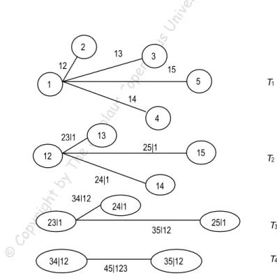
(5) Modeling the Dependence Structure of the WIG20 Portfolio Using a Pair-copula…. 35. 2. icu sU. niv er. sit y. Sc. ien. tif. ic. Pu b. lis. hin. gH. ou. se. Decompositions such as (14) and (15) are called pair-copula constructions. In fact, for high-dimensional distributions there are many possible pair-copula decompositions. Some methods that help organize them are described by Bedford and Cooke (2001, 2002) in the language of the so-called regular vines. In what follows, we use some very basic notions concerning graphs, which can be found, for instance, in (Kurowicka, Cooke, 2006). We start with the definition of a regular vine on n variables. It is the structure composed of n − 1 trees (T1 ,…, Tn ) in which T1 is a tree with the set of nodes N1 = {1,…, n} and the set of edges E1 , and for i = 2,… , n − 1 , the Ti is a tree with the set of nodes Ni = Ei −1 . Moreover, it should hold that if some nodes a = {a1 , a2 } , b = {b1 , b2 } are connected by an edge then exactly one ai is equal to exactly one bi . In financial applications, the most important are two special cases of regular vines: canonical vines and the D-vines. A regular vine is called a canonical vine (or C-vine) if in each tree Ti (i < n − 1) there exists exactly one node with degree n − i . The node in T1 that has maximal degree is called the root. A regular vine is called a D-vine if each node in T1 has a degree of at most 2. Examples of C- and D-vines are shown in Figures 1 and 2.. 13. 3. op er n. 12. 15 5. T1. sC. 1. 13. 25|1. 15. Th. rig ht Co py ©. 4. 24|1. by. 12. eN. 23|1. ico lau. 14. 34|12. 14 24|1. 23|1. 34|12. T2. 35|12. 45|123. Figure 1. A canonical vine on 5 variables. 35|12. 25|1. T3 T4.

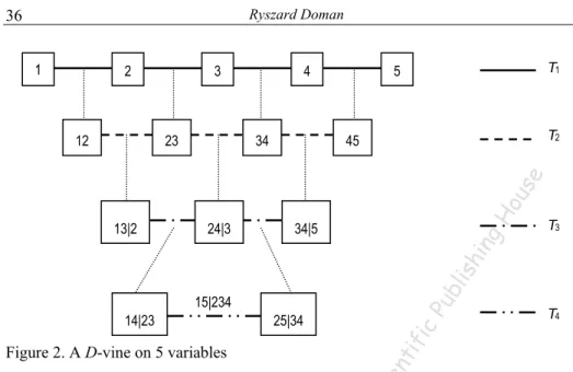
(6) Ryszard Doman. 36 1. 2. 3. 23. 34. T1. 5. T2. 45. 24|3. 34|5. T3. Pu b. lis. hin. 13|2. gH. ou. se. 12. 4. 15|234. T4. ic. 25|34. tif. 14|23. ien. Figure 2. A D-vine on 5 variables. niv er. sit y. Sc. It is not very hard to observe that formula (14) gives a pair-copula construction corresponding to a canonical vine, and formula (15) defines a pair-copula construction that can be described by a D-vine. It should be mention here that starting from n nodes one can construct n !/ 2 different canonical vines and n !/ 2 different D-vines (Aas et al., 2009). When some components X i and X j. icu sU. of the vector X are conditionally independent given a subvector V of X then ci , j|v ( F ( xi | v ), F ( x j | v )) = 1 , and thus the pair-copula decomposition in (14) or. Th. eN. ico lau. sC. op er n. (15) simplifies. This property is of great importance from a practical point of view. It shows how a careful selection of variables and a proper choice of their ordering can affect the model complexity. The canonical vines and D-vines can be estimated by maximum likelihood method. If we assume that the data xt = ( x1,t ,…, xn,t ) , t = 1,… , T , are observations of variables that are independent over time then the log-likelihood for the canonical vine is given by n −1 n − j T. by. L( x; Θ) = ∑∑∑ log[c j , j +i|1,…, j −1 ( F ( x j ,t | x1,t ,…, x j −1,t ),. rig ht. j =1 i =1 t =1. (16). Co py. F ( x j +i ,t | x1,t ,…, x j −1,t ); Θ j ,i )] ,. ©. and for the D-vine it has the form n n− j T. L( x, Θ) = ∑∑∑ log[ci ,i + j|i +1,…,i + j −1 ( F ( xi ,t | xi +1,t ,…, xi + j −1,t ), j =1 i =1 t =1. F ( xi + j ,t | xi +1,t …, xi + j −1,t );Θi , j ))] .. (17).

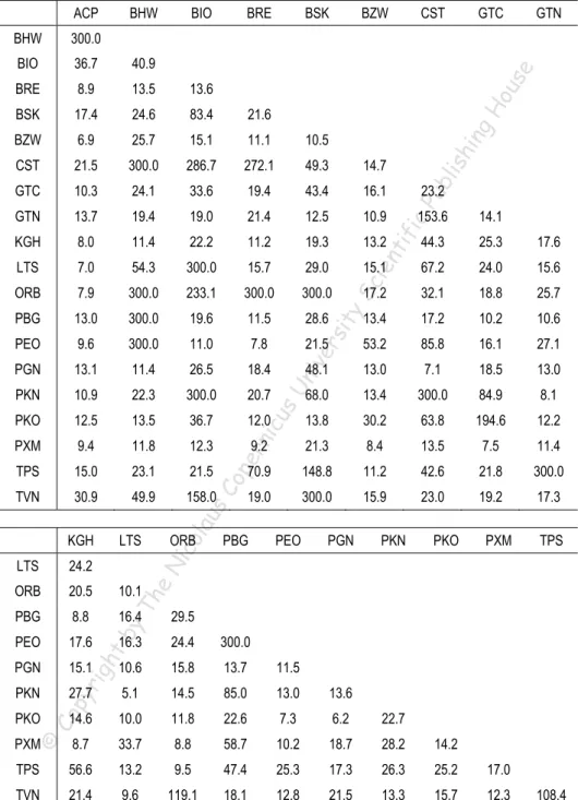
(7) Modeling the Dependence Structure of the WIG20 Portfolio Using a Pair-copula…. 37. gH. ou. se. The number of parameters depends on copula types used in the model specification. In the presence of temporal dependence, as is in the case of real data, usually some ARMA-GARCH models are fitted to the margins, and the estimation is performed for the standardized residuals. Thus in fact, the estimation method is that of maximum pseudo-likelihood. The consistency and asymptotic normality of the estimators obtained in such a way is discussed by Genest et al. (1995) and Joe (1997).. hin. 4. The Data and Model Specification. rig ht. by. Th. eN. ico lau. sC. op er n. icu sU. niv er. sit y. Sc. ien. tif. ic. Pu b. lis. The data we use in this paper consist of daily returns on the stocks of the companies that constituted the WIG20 index of the Warsaw Stock Exchange during the period from September 23, 2005 to May 29, 2009.The tickers of the securities under scrutiny are as follows: ACP, BHW, BIO, BRE, BSK, BZW, CST, GTC, GTN, KGH, LTS, ORB, PBG, PEO, PGN, PKN, PKO, PXM, TPS, TVN. The returns are calculated as rt = 100(ln Pt − ln Pt −1 ) , where Pt is the closing quotation on day t. The return series showed some autocorrelation and in all cases conditional homoskedasticity was strongly rejected by the Engle test. Following a commonly accepted approach, we first estimated the ARMA-GJR-GARCH models for the marginal returns. In each case a standardized skewed Student’s t distribution (Lambert, Laurent, 2001) was applied as the error distribution. Next, the standardized residuals series were transformed into uniform on [0,1] by using the corresponding probability integral transforms. For the transformed data, we estimated a D-vine, described by the decomposition (15). Prior to choosing an ordering of the univariate series we estimated a bivariate Student’s t copula for each of the possible 190 pairs. Next, we analyzed the pairs with respect the estimated number of degrees of freedom, which was assumed to be a risk factor. We decided to apply bivariate Student’s t copulas for all pairs in estimated pair-copula decomposition. The final ordering of the marginal univariate series was chosen in such a way that the numbers of degrees of freedom of copulas connecting the consecutive series in tree 1 of the D-vine formed a non-decreasing sequence.. Co py. 5. Empirical Results. ©. In applications of pair-copula constructions it is of great importance to carefully consider the selection of specific factorization, and the choice of bivariate copula types. Thus in the first stage of our investigation we tried to fit bivariate copulas of diverse type to each of the possible pairs of the series from our dataset. Finally we decided to use Student’s t copulas, and focus on their numbers of degrees of freedom considered as risk factors. The obtained estimates of the numbers of degrees of freedom are presented in Table 1..

(8) Table 1. Estimates for the number of degrees of freedom in bivariate Student’s t copulas fitted to the pairs of the return series, period Sept. 23, 2005 – May 29, 2009. 40.9. BRE. 8.9. 13.5. CST. GTC. GTN. 13.6. ou. 36.7. BZW. 17.4. 24.6. 83.4. 21.6. 6.9. 25.7. 15.1. 11.1. 10.5. CST. 21.5. 300.0. 286.7. 272.1. 49.3. 14.7. GTC. 10.3. 24.1. 33.6. 19.4. 43.4. 16.1. GTN. 13.7. 19.4. 19.0. 21.4. 12.5. 10.9. KGH. 8.0. 11.4. 22.2. 11.2. 19.3. 13.2. 44.3. 25.3. 17.6. LTS. 7.0. 54.3. 300.0. 15.7. 29.0. 15.1. 67.2. 24.0. 15.6. ORB. 7.9. 300.0. 233.1. 300.0. 300.0. 32.1. 18.8. 25.7. PBG. 13.0. 300.0. 19.6. 11.5. 28.6. 13.4. 17.2. 10.2. 10.6. PEO. 9.6. 300.0. 11.0. 7.8. 21.5. 53.2. 85.8. 16.1. 27.1. PGN. 13.1. 11.4. 26.5. 18.4. 13.0. 7.1. 18.5. 13.0. PKN. 10.9. 22.3. 300.0. 20.7. 68.0. 13.4. 300.0. 84.9. 8.1. PKO. 12.5. 13.5. 36.7. 12.0. 13.8. 30.2. 63.8. 194.6. 12.2. PXM. 9.4. 11.8. 12.3. 9.2. 21.3. 8.4. 13.5. 7.5. 11.4. TPS. 15.0. 23.1. 21.5. 70.9. 148.8. 11.2. 42.6. 21.8. 300.0. TVN. 30.9. 49.9. 158.0. 19.0. 300.0. 15.9. 23.0. 19.2. 17.3. ORB. icu sU. PBG. PEO. lis Pu b ic. 153.6. tif. sit y. 17.2. 48.1. op er n. sC. ico lau. LTS. 23.2. PGN. PKN. PKO. 14.1. PXM. 24.2 20.5. 10.1. PBG. 8.8. 16.4. 29.5. PEO. 17.6. 16.3. 24.4. 300.0. PGN. 15.1. 10.6. 15.8. 13.7. 11.5. PKN. 27.7. 5.1. 14.5. 85.0. 13.0. 13.6. 14.6. 10.0. 11.8. 22.6. 7.3. 6.2. 22.7. PXM. 8.7. 33.7. 8.8. 58.7. 10.2. 18.7. 28.2. 14.2. TPS. 56.6. 13.2. 9.5. 47.4. 25.3. 17.3. 26.3. 25.2. 17.0. TVN. 21.4. 9.6. 119.1. 18.1. 12.8. 21.5. 13.3. 15.7. 12.3. Th. rig ht. Co py. ©. PKO. TPS. eN. LTS ORB. by. KGH. hin. BSK BZW. ien. BIO. BSK. Sc. 300.0. BRE. niv er. BHW. BIO. se. BHW. gH. ACP. 108.4. Note: We estimated the number of degrees of freedom parameter subject to upper bound equal to 300. In practice, the value 300 means that the Gaussian copula is the proper one..

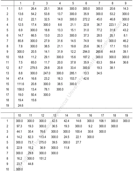
(9) Modeling the Dependence Structure of the WIG20 Portfolio Using a Pair-copula…. 39. 2. 3. 4. 5. 6. 7. 8. 9. 5.1. 26.4. 25.1. 38.6. 300.0. 300.0. 300.0. 20.6. 14.3. 2. 13.6. 54.2. 53.8. 13.7. 300.0. 35.9. 300.0. 53.2. 300.0. 3. 6.2. 22.1. 32.5. 14.0. 300.0. 272.2. 45.0. 46.8. 300.0. 4. 12.5. 17.4. 300.0. 8.6. 21.1. 22.8. 36.7. 223.1. 24.2. 5. 6.9. 300.0. 18.8. 13.3. 15.1. 31.0. 77.2. 31.8. 43.2. 6. 14.7. 66.5. 13.0. 23.3. 300.0. 37.3. 28.5. 20.1. 8.1. 7. 85.8. 300.0. 27.9. 31.6. 14.5. 74.9. 18.0. 300.0. 46.2. 8. 7.8. 300.0. 38.5. 21.1. 19.8. 25.6. 36.1. 17.1. 15.0. 9. 300.0. 20.5. 14.1. 31.9. 12.2. 294.0. 260.6. 44.8. 39.1. 10. 18.8. 11.2. 29.1. 300.0. 15.6. 187.2. 300.0. 11. 7.5. 65.0. 11.7. 20.0. 37.8. 35.9. 12. 8.7. 279.5. 29.8. 20.8. 33.4. ien. 13. 8.8. 300.0. 247.0. 300.0. 285.1. 14. 47.4. 16.6. 23.2. 16.3. 153.7. 42.6. 15. 111.6. 20.8. 300.0. 38.5. 300.0. 16. 158.0. 13.4. 78.1. 300.0. 17. 19.0. 50.4. 300.0. 18. 19.4. 15.6. 19. 24.6 10. 11. 12. 1. 300.0. 300.0. 300.0. 2. 97.3. 19.3. ou. gH. hin. lis. Pu b. 38.1. tif. ic. 19.3 34.5. op er n. icu sU. niv er. sit y. 13.3. 15. 16. 17. 18. 19. 300.0. 108.1. 300.0. 300.0. 300.0. 36.5. 19.3. 300.0. 9.2. 300.0. 300.0. 76.6. 300.0. 300.0. 100.4. 30.6. 300.0. 113.4. 300.0. 24.5. 22.1. 300.0. 27.7. ico lau. 5. 300.0. 73.7. 275.0. 39.5. 300.0. 6. 22.9. 15.2. 36.9. 300.0. 11.8. 7. 300.0. 29.8. 300.0. 300.0. 8. 16.2. 300.0. 9. 23.7. 44.8. eN. 30.4 82.3. Th. 300.0. 14.6. 44.1. by. 36.6. 14. 14.2. rig ht. 300.0. 59.4. 42.4. sC. 13. 4. Co py. 300.0. 63.3. 42.5. 3. 10. se. 1 1. Sc. Table 2. Estimates for the number of degrees of freedom in the fitted D-vine. 151.2. 300.0. ©. Note: The numbers of degrees of freedom for the copulas appearing in trees 1-19 of the estimated D-vine are presented in columns. We estimated the number of degrees of freedom parameter subject to upper bound equal to 300. In practice, the value 300 means that the Gaussian copula is the proper one.. We used the obtained estimates of the number of degrees of freedom for the bivariate return series to chose an efficient ordering of the variables included in.

(10) Ryszard Doman. 40. Th by. w1 = u1 ,. eN. ico lau. sC. op er n. icu sU. niv er. sit y. Sc. ien. tif. ic. Pu b. lis. hin. gH. ou. se. the decomposition (15). Our choice was the following: 1. LTS, 2. PKN, 3. PGN, 4. PKO, 5. ACP, 6. BZW, 7. CST, 8. PEO, 9. BRE, 10. ORB, 11. GTC, 12. PXM, 13. KGH, 14. PBG, 15. TPS, 16. TVN, 17. BIO, 18. GTN, 19. BHW, 20. BSK. The motivation was that in that case, for the 19 bivariate copulas fitted to the pairs of the returns in accordance to the formula of tree 1 of the estimated D-vine, the sequence of the corresponding numbers of degrees of freedom is non-decreasing. The D-vine estimation results are presented in table 2. For a comparison we fitted to the investigated vector return series a standard 20-dimensional Student’s t copula. As an estimate for the number of degrees of freedom we obtained 34.4265. Looking at the estimates for the bivariate copulas in tree 1 of the estimated D-vine, which vary from 5.1 to 300, we can state that the superiority of the pair-copula construction approach over the standard multidimensional copula approach is strongly supported. A significantly better fit of the D-vine model has been also indicated by the Akaike information criterion. Our next objective was to use the estimated D-vine to compute in-sample VaR estimates for long and short positions (Giot, Laurent, 2003) for the portfolio composed of the considered stocks, and compare them to the ones obtained by using Engle’s (2002) DCC model with multivariate Student’s t distribution. In the DCC model case we could use the well-known formulas for a portfolio VaR (see e.g. Giot, Laurent, 2003), having the estimates of the conditional covariances and the degree of freedom for the conditional Student’s t distribution, which was estimated as 13.7881. For the approach using the pair-copula construction, we simulated for each day 1000 20-dimensional vectors from the fitted D-vine. Then we transformed them into the one-dimensional standardized residuals, and, finally, into the daily returns of the portfolio components. After that we obtained the daily VaR estimates as the corresponding quantiles. The VaR calculation was performed for significance levels 0.01, 0.025, and 0.05. An algorithm for sampling from an n-dimensional D-vine proceeds as follows (see Aas et al., 2009). Start with sampling variates u1 ,…, un independent uniform on [0, 1]. Then set. rig ht. w2 = F −1 (u2 | w1 ) ,. Co py. w3 = F −1 (u3 | w1 , w2 ) ,. ©. wn = F −1 (un | w1 ,…, wn −1 ) .. The general formula for the functions F ( x j | x1 ,…, x j −1 ) involves (12) and (13), and it is given in the paper by Aas et al. (2009), where one can also find explicit formulas for the inverse in the case in which all the bivariate copulas of a pair copula construction are Student’s t copulas..

(11) Moddeling the Depeendence Structuure of the WIG2 20 Portfolio Usiing a Pair-copuula…. 41. sit y. Sc. ien. tif. ic. Pu b. lis. hin. gH. ou. se. Our results r conceerning in-sam mple VaR callculation aree not unambiguous. To assess thee quality of the VaR esttimates we applied a the coverage c andd independence tessts by Chrisstoffersen (1998). Generrally speakinng, we obtaained very good resuults for longg trading possitions, and rather poor results for sshort positions. Foor long posittions, howevver, the pairr-copula moodel outperfoormed the DCC model definitelly, especiallyy at tolerance level 0.05 where the pp-value of the coverrage test waas close to 1. 1 The resultts corresponnding to this tolerance level are shown in Figgures 1 and 2. 2. eN. ico lau. sC. op er n. icu sU. niv er. Figure 1. In-sample VaR V calculatedd by means of o the fitted pair-copula p coonstruction. Tolerance leevel equal to 0.05 0. by. Th. Figure 2. In-sample VaR V calculatedd by means of Engle’s DC CC model withh Student’s t conditionall distribution. Tolerance lev vel equal to 0.05. rig ht. 5. Concclusions. ©. Co py. In thiis paper we applied a the pair-copula p construction c methodologgy to modeling the dependence structure off the returns on stocks coonstituting thhe WIG20 index. We W focused onn the numbeer of degreess of freedom m of the bivaariate Student’s t copulas c entering the connstruction, co onsidering itt as a risk faactor. The results off our investiigation show w that the raange of the estimates e caan be very large. Thhis fact suppports usefulnness of the new methoddology and pproves its superioritty over the classical c appproaches. In addition, wee used the ffitted paircopula coonstruction for f simulation from the joint multidim mensional diistribution of the WIIG20 index portfolio, p and applied thee simulation output for ccalculating.

(12) Ryszard Doman. 42. Value-at-Risk. Our results show that the VaR estimates for long trading positions at tolerance level 0.05 obtained in this way definitely outperform the ones calculated by using a fitted DCC model with Student’s t conditional distribution.. ou. se. References. by. Th. eN. ico lau. sC. op er n. icu sU. niv er. sit y. Sc. ien. tif. ic. Pu b. lis. hin. gH. Aas, K., Czado, C., Frigessi, A., Bakken, H. (2009), Pair-Copula Constructions of Multiple Dependence, Insurance: Mathematics and Finance, 44, 182–198. Bauwens, E. Laurent, S. Rombouts, J.V.K. (2006), Multivariate GARCH Models: A Survey, Journal of Applied Econometrics, 21, 79–109. Bedford, T., Cooke, R.M. (2001), Probability Density Decomposition for Conditionally Dependent Random Variables Modeled by Vines, Annals of Mathematics and Artificial Intelligence, 32, 245–268. Bedford, T., Cooke, R.M. (2002), Vines – a New Graphical Model for Dependent Random Variables, Annals of Statistics, 30, 1031–1068. Christoffersen, P. F. (1998), Evaluating Interval Forecasts, International Economic Review, 39, 841–862. Engle, R. F., (2002), Dynamic Conditional Correlation: A Simple Class of Multivariate Generalized Autoregressive Conditional Heteroskedasticity Models, Journal of Business & Economic Statistics, 20, 339–350. Genest, C. Ghoudi K. Rivest, L.-P. (1995), A Semiparametric Estimation Procedure of Dependence Parameters in Multivariate Families of Distributions, Biometrika, 82, 543–552. Giot, P., Laurent, S. (2003), Value-at-Risk for Long and Short Trading Positions, Journal of Applied Econometrics, 18, 641–664. Joe, H. (1996), Families of m-variate Distributions with Given Margins and m(m - 1)/2 Bivariate Dependence Parameters. In: Rüschendorf, L., Schweizer, B.,Taylor, M.D. (Eds.), Distributions with Fixed Marginals and Related Topics, IMS Lecture Notes Monograph Series 28, Institute of Mathematical Statistics, Hayward, CA, 120–141. Joe, H. (1997), Multivariate Models and Dependence Concepts, Chapman & Hall, London. Kurowicka, D., Cooke, R. M., (2006), Uncertainty Analysis with High Dimensional Dependence Modelling, Wiley, New York. Lambert, P., Laurent, S. (2001), Modelling Financial Time Series Using GARCH-type Models with a Skewed Student Distribution for the Innovations, Institut de Statistique, Université Catholique de Louvain, Discussion Paper 0125. Nelsen, R. B. (2006) An Introduction to Copulas (2nd ed.), Springer, New York Sklar, A. (1959), Fonctions de rérpartition à n dimensions et leurs marges, Publications de l’Institut Statistique de l’Université de Paris, 8, 229–231.. Co py. rig ht. Modelowanie struktury zależności portfela indeksu WIG20 za pomocą kaskady kopuli dwuwymiarowych. ©. Z a r y s t r e ś c i. W artykule przedstawiono wyniki zastosowania nowej metodologii modelowania zależności pomiędzy zwrotami składników portfela wysokowymiarowego. Idea tego podejścia polega na dekompozycji gęstości rozkładu łącznego na iloczyn, w którym występują jedynie gęstości kopuli dwuwymiarowych pewnych rozkładów warunkowych wyznaczonych przez modelowane zmienne. Badania dotyczą stóp zwrotu z akcji wchodzących w skład indeksu WIG20 i potwierdzają pewną przewagę nowej metodologii nad podejściem, w którym stosowany jest model DCC Engle’a z wielowymiarowym rozkładem t Studenta. S ł o w a k l u c z o w e: zależność, portfel, kopula, kaskada kopuli dwuwymiarowych..

(13)

No results found