Theses & Dissertations Boston University Theses & Dissertations
2017
Evaluating multiple imputation
methods for longitudinal healthy
aging index - a score variable with
data missing due to death, dropout
and several missing data
mechanisms
https://hdl.handle.net/2144/27352 Boston UniversityGRADUATE SCHOOL OF ARTS AND SCIENCES
Dissertation
EVALUATING MULTIPLE IMPUTATION METHODS FOR LONGITUDINAL HEALTHY AGING INDEX – A SCORE VARIABLE WITH DATA MISSING DUE
TO DEATH, DROPOUT AND SEVERAL MISSING DATA MECHANISMS
by
ELIZABETH L. KANE
B.A., Hartwick College, 2006 M.S., University of Rhode Island, 2008
Submitted in partial fulfillment of the requirements for the degree of
Doctor of Philosophy 2017
© Copyright by
ELIZABETH L KANE 2017
All rights reserved except for Chapter 2, which is ©2016 by Oxford University Press. The full article, Association of an Index of Healthy Aging With Incident Cardiovascular Disease and Mortality in a Community-Based Sample of Older Adults by Elizabeth L. McCabe, Martin G. Larson, Kathryn L. Lunetta, Anne B. Newman, Susan Cheng, Joanne M. Murabito; ©2016, reproduced by permission of Oxford University.
http://biomedgerontology.oxfordjournals.org/cgi/ content/abstract/glw077?ijkey=sczt52voaFo4yl9 &keytype=ref
Approved by First Reader ____________________________________________________ Martin G. Larson, ScD Professor of Biostatistics Second Reader ____________________________________________________ Joseph M. Massaro, PhD Professor of Biostatistics Third Reader ____________________________________________________ Kathryn L. Lunetta, PhD Professor of Biostatistics
iv
ACKNOWLEDGEMENTS
I wish to thank my thesis advisor, Marty Larson, for being a great mentor and sharing all of his knowledge of statistics and grammar. Thank you to my
committee: Joe Massaro, Kathy Lunetta, Susan Cheng and Tim Heeren. A special thank you to Susan for her funding support throughout my time at BU. I would also like to thank Joanne Murabito for taking the senior author position on my HAI paper, and for all her mentoring and patience while I learned how to prepare a manuscript for publication.
Finally, I would like to thank my family and friends. To my parents: thank you for always supporting me and believing in me. Thank you for teaching me to set goals and helping me realize I can achieve them. Thank you, Phil, for being patient with me over the past several years. Your love and support was imperative for my success. To Heather: thank you for being my birdie, and for being here for every step of the process – I could never have done this without you. To the rest of my family, BU friends, dinner club and everyone else – thank you for your support. I love you all and I appreciate you keeping me grounded while I embarked on this crazy and wild ride.
v
EVALUATING MULTIPLE IMPUTATION METHODS FOR LONGITUDINAL HEALTHY AGING INDEX – A SCORE VARIABLE WITH DATA MISSING DUE
TO DEATH, DROPOUT AND SEVERAL MISSING DATA MECHANISMS
ELIZABETH L. KANE
Boston University Graduate School of Arts and Sciences, 2017
Major Professor: Martin G. Larson, Professor of Biostatistics
ABSTRACT
The healthy aging index (HAI) is a score variable based on five clinical components. I assess how well it predicts mortality in a sample of older adults from the Framingham Heart Study (FHS). Over 30% of FHS participants have missing HAI across time; I investigate how well imputation methods perform in this setting. I run simulations to compare four methods of multiple imputation (MI) by fully conditional specification (FCS) and the complete case (CC) approach on estimation of means, correlations, and slopes of the HAI over time. I simulate multivariate normal data for each component of HAI at four time points, along with age and sex, using within and across-time correlation patterns at the percent of missing data seen in observed FHS data. My methods of MI are
cross-sectional FCS (XFCS, imputation model uses other components at same time), longitudinal FCS (LFCS, uses same component at all times ignoring
cross-vi
component correlation), all FCS (AFCS, uses all components at all times) and 2-fold FCS (2fFCS, uses all components at current and adjacent times). I compare percent bias, confidence interval width, coverage probability and relative
efficiency for three mechanisms of missing data (MCAR,MAR,MNAR), two sample sizes (n=1000,100), and two numbers of imputed datasets (m=5,20). All longitudinal methods (not XFCS) yield nearly identical results with unbiased estimates of means, correlations and slopes. Increase in precision and relative efficiency is small when augmenting from 5 to 20 imputations.
Finally, I compare the imputation methods and CC analysis in survival models using HAI as a time-dependent variable to predict mortality. I simulate HAI data as described above, time-to-death using piece-wise exponential models, and I impose type I and random censoring on 32% of observations. CC analysis
reduces sample size by 10%, produces unbiased estimates, but inflates standard errors. The three longitudinal imputation methods introduce minimal bias (<5%) in the hazard ratio estimates, while reducing the standard error up to 10% compared with CC.
Overall, I show that multiple imputation using longitudinal methods is
beneficial in the setting of repeated measurements of a score variable. It works well in analyzing changes over time and in time-dependent survival analyses.
vii
TABLE OF CONTENTS
ACKNOWLEDGEMENTS ...iv
ABSTRACT ... v
TABLE OF CONTENTS ... vii
LIST OF TABLES ... x
LIST OF FIGURES ... xiii
LIST OF ABBREVIATIONS ... xxi
CHAPTER 1 - INTRODUCTION ... 1
Missing Data ... 1
Healthy Aging Index ... 2
Literature Review ... 4
Thesis ... 13
CHAPTER 2 – HEALTHY AGING INDEX IN THE FRAMINGHAM HEART STUDY: A MOTIVATING EXAMPLE ... 15
Introduction ... 15
Methods ... 16
Results ... 23
Discussion ... 27
viii
Figures ... 41
CHAPTER 3 – MEANS, CORRELATIONS AND SLOPES ... 45
Introduction ... 45 Methods ... 46 Results ... 54 FHS Application ... 66 Discussion ... 68 Tables ... 70 Figures ... 82
CHAPTER 4 – SURVIVAL MODELS ... 127
Introduction ... 127 Methods ... 128 Results ... 132 FHS Application ... 135 Discussion ... 135 Tables ... 141 Figures ... 146 CHAPTER 5 ... 156 BIBLIOGRAPHY ... 160
ix
x
LIST OF TABLES
Table 1. Cut-points Used to Group Each Component of the HAI... 30
Table 2. Variables Used to Impute Each HAI Component and Covariates ... 31
Table 3. Sample Characteristics ... 32
Table 4. Associations of Modified HAI with All-Cause Mortality ... 33
Table 5. Numbers of Events and Sample Size per Category of HAI... 34
Table 6. Associations of Modified HAI with CVD ... 35
Table 7. Association between HAI and Cancer ... 36
Table 8. Spearman Correlations of HAI Components with Other Markers of Aging ... 37
Table 9. Associations of Other Markers of Aging with Mortality and CVD in Sample with Complete HAI Data ... 38
Table 10. C-Statistics for Models Including Original and Modified HAI ... 39
Table 11. Associations in Imputed Data Between HAI and All-Cause-Mortality and CVD ... 40
Table 12. Target Correlation Matrix ... 70
xi
Table 14. Thresholds Used to Group Each Component of the HAI ... 72
Table 15. Target Percent of Missing Values ... 73
Table 16. Mean HAI in Full Simulated Data ... 74
Table 17. Correlation of HAI across Exams in Full Simulated Data ... 75
Table 18. Percent Missing Values in Full Simulated Data ... 76
Table 19. Potential Scale Reduction Factor (𝑹𝒄) for Imputed Values for Means, Correlations and Slopes ... 77
Table 20. Mean HAI in Complete Case and Imputed Data in FHS ... 78
Table 21. Correlation of HAI in Complete Case and Imputed FHS Data ... 79
Table 22. Slope of Linear Mixed Effect Model Estimating Change in HAI over Time in Complete Case and Imputed FHS Data ... 80
Table 23. Computation Times for Multiple Imputation Methods in Framingham Heart Study Data ... 81
Table 24. Comparing Complete Case Analysis vs. Last Observation Carried Forward Methods in Time-Dependent Survival Models ... 141
Table 25. Coverage Probabilities for Estimates of Log Hazard Ratio in Imputed Data ... 142
xii
Table 26. Potential Scale Reduction Factor (𝑹𝒄) to Assess Convergence in Imputations for Time-Dependent Survival Analyses ... 143 Table 27. Results from Multiple Imputation Methods in FHS Data for
Time-Dependent Survival Analysis ... 144 Table 28. Computation Times for Multiple Imputation Methods in Framingham Heart Study Data ... 145
xiii
LIST OF FIGURES
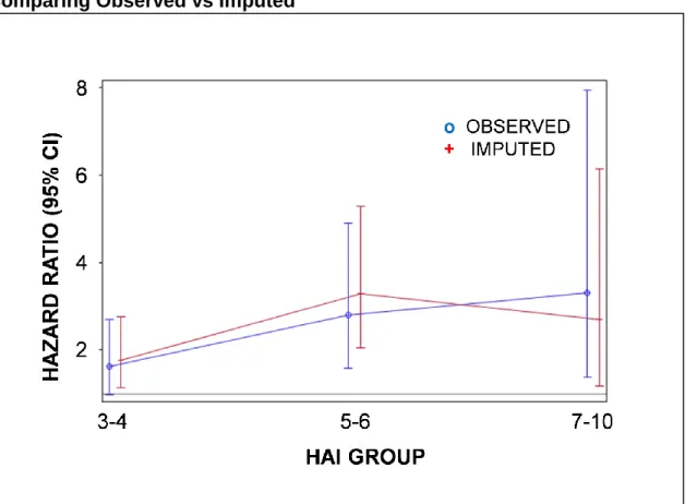
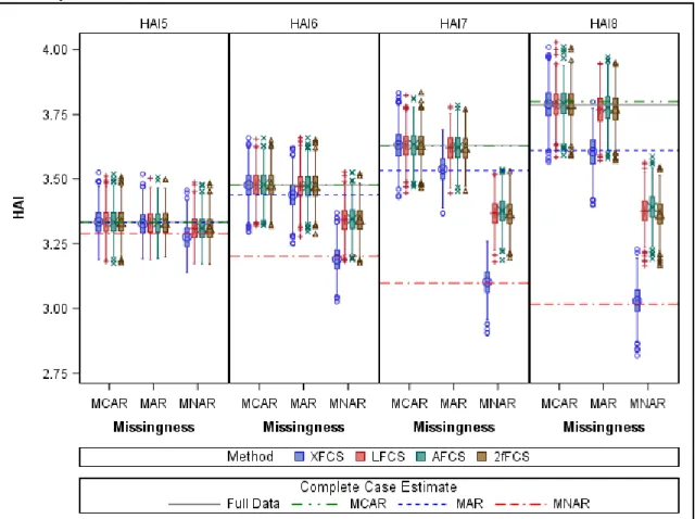
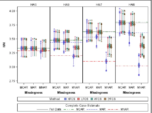
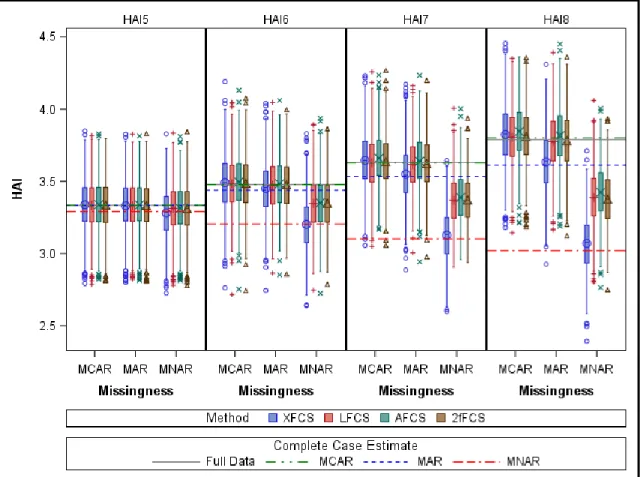
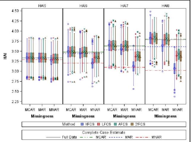
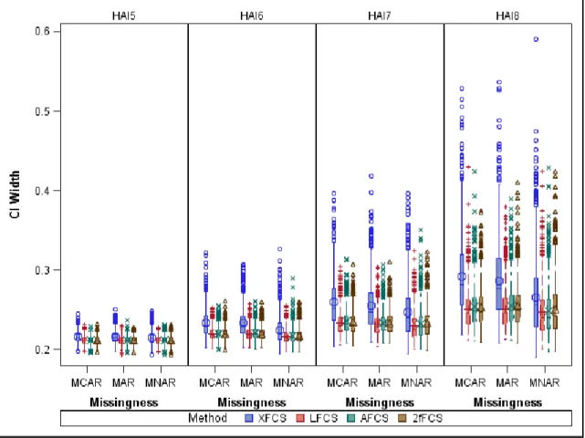
Figure 1. Histograms of Healthy Aging Index and Self-Reported Health at Exam 5 (n=934) ... 41 Figure 2. Side-by-side Boxplots of HAI by Self-Reported Health ... 42 Figure 3. Hazard Ratio for All-Cause Mortality by HAI Group in Multivariable Models Comparing Observed vs Imputed ... 43 Figure 4. Hazard Ratio for CVD by HAI Group in Multivariable Models Comparing Observed vs Imputed ... 44 Figure 5. Mean HAI across Exams for Different Missing Data Mechanisms and Imputation Methods with N=1000 and m=5 ... 82 Figure 6. Mean HAI across Exams for Different Missing Data Mechanisms and Imputation Methods with N=1000 and m=20 ... 83 Figure 7. Mean HAI across Exams for Different Missing Data Mechanisms and Imputation Methods with N=100 and m=5 ... 84 Figure 8. Mean HAI across Exams for Different Missing Data Mechanisms and Imputation Methods with N=100 and m=20 ... 85 Figure 9. Confidence Interval Width for Mean HAI across Exams for Different Missing Data Mechanisms and Imputation Methods with N=1000 and m=5 ... 86
xiv
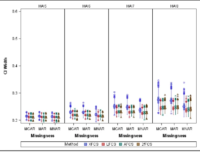
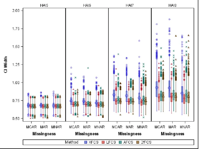
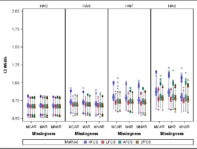
Figure 10. Confidence Interval Width for Mean HAI across Exams for Different Missing Data Mechanisms and Imputation Methods with N=1000 and m=20 .... 87 Figure 11. Confidence Interval Width for Mean HAI across Exams for Different Missing Data Mechanisms and Imputation Methods with N=100 and m=5 ... 88 Figure 12. Confidence Interval Width for Mean HAI across Exams for Different Missing Data Mechanisms and Imputation Methods with N=100 and m=20 ... 89 Figure 13. Coverage Probability of Confidence Intervals for Mean HAI across Exams for Different Missing Data Mechanisms and Imputation Methods with N=1000 and m=5 ... 90 Figure 14. Coverage Probability of Confidence Intervals for Mean HAI across Exams for Different Missing Data Mechanisms and Imputation Methods with N=1000 and m=20 ... 91 Figure 15. Coverage Probability of Confidence Intervals for Mean HAI across Exams for Different Missing Data Mechanisms and Imputation Methods with N=100 and m=5 ... 92 Figure 16. Coverage Probability of Confidence Intervals for Mean HAI across Exams for Different Missing Data Mechanisms and Imputation Methods with N=100 and m=20 ... 93
xv
Figure 17. Relative Efficiency for Mean HAI across Exams for Different Missing Data Mechanisms and Imputation Methods with N=1000 and m=5... 94 Figure 18. Relative Efficiency for Mean HAI across Exams for Different Missing Data Mechanisms and Imputation Methods with N=1000 and m=20... 95 Figure 19. Relative Efficiency for Mean HAI across Exams for Different Missing Data Mechanisms and Imputation Methods with N=100 and m=5... 96 Figure 20. Relative Efficiency for Mean HAI across Exams for Different Missing Data Mechanisms and Imputation Methods with N=100 and m=20... 97 Figure 21. Percent Missing Data and Relative Efficiency of Mean of HAI across Exams in Samples of n=1000 ... 98 Figure 22. Correlation of HAI across Exams in Samples of n=1000 and Data Imputed with m=5 ... 99 Figure 23. Alternate View of Correlation of HAI across Exams in Samples of n=1000 and Data Imputed with m=5 ... 100 Figure 24. Correlation of HAI across Exams in Samples of n=1000 and Data Imputed with m=20 ... 101 Figure 25. Correlation of HAI across Exams in Samples of n=100 and Data Imputed with m=5 ... 102
xvi
Figure 26. Correlation of HAI across Exams in Samples of n=100 and Data Imputed with m=20 ... 103 Figure 27. Comparing 2fFCS with Time Window Width of One Exam vs Two Exams ... 104 Figure 28. Confidence Interval Width of Correlation of HAI across Exams in Samples of n=1000 and Data Imputed with m=5 ... 105 Figure 29. Alternate View of Confidence Interval Width of Correlation of HAI across Exams in Samples of n=1000 and Data Imputed with m=5... 106 Figure 30. Confidence Interval Width of Correlation of HAI across Exams in Samples of n=1000 and Data Imputed with m=20 ... 107 Figure 31. Confidence Interval Width of Correlation of HAI across Exams in Samples of n=100 and Data Imputed with m=5 ... 108 Figure 32. Confidence Interval Width of Correlation of HAI across Exams in Samples of n=100 and Data Imputed with m=20 ... 109 Figure 33. Coverage Probability of Confidence Intervals for Correlation of HAI across Exams for Different Missing Data Mechanisms and Imputation Methods with N=1000 and m=5 ... 110
xvii
Figure 34. Coverage Probability of Confidence Intervals for Correlation of HAI across Exams for Different Missing Data Mechanisms and Imputation Methods with N=1000 and m=20 ... 111 Figure 35. Coverage Probability of Confidence Intervals for Correlation of HAI across Exams for Different Missing Data Mechanisms and Imputation Methods with N=100 and m=5 ... 112 Figure 36. Coverage Probability of Confidence Intervals for Correlation of HAI across Exams for Different Missing Data Mechanisms and Imputation Methods with N=100 and m=20 ... 113 Figure 37. Relative Efficiency of Correlation of HAI across Exams in Samples of n=1000 and Data Imputed with m=5 ... 114 Figure 38. Relative Efficiency of Correlation of HAI across Exams in Samples of n=1000 and Data Imputed with m=20 ... 115 Figure 39. Relative Efficiency of Correlation of HAI across Exams in Samples of n=100 and Data Imputed with m=5 ... 116 Figure 40. Relative Efficiency of Correlation of HAI across Exams in Samples of n=100 and Data Imputed with m=20 ... 117 Figure 41. Percent Missing Data and Relative Efficiency of Correlation of HAI across Exams in Samples of n=1000 ... 118
xviii
Figure 42. Slope of Linear Mixed Effects Models for HAI across Exams in
Samples of n=1000 ... 119 Figure 43. Slope of Linear Mixed Effects Models for HAI across Exams in
Samples of n=100 ... 120 Figure 44. Confidence Interval Width for Slope of Linear Mixed Effects Models for HAI across Exams in Samples of n=1000 ... 121 Figure 45. Confidence Interval Width for Slope of Linear Mixed Effects Models for HAI across Exams in Samples of n=100 ... 122 Figure 46. Coverage Probability of Confidence Intervals for Slope of Linear Mixed Effects Models for HAI across Exams for Different Missing Data Mechanisms and Imputation Methods with N=1000 ... 123 Figure 47. Coverage Probability of Confidence Intervals for Slope of Linear Mixed Effects Models for HAI across Exams for Different Missing Data Mechanisms and Imputation Methods with N=100 ... 124 Figure 48. Relative Efficiency for Slope of Linear Mixed Effects Models for HAI across Exams with m=5 ... 125 Figure 49. Relative Efficiency for Slope of Linear Mixed Effects Models for HAI across Exams with m=20 ... 126
xix
Figure 50. Cumulative Distribution Function for Censoring Time in Random Censoring ... 146 Figure 51. Comparing Type I Censoring to Random Censoring for Parameter Estimates of Time-Dependent HAI in Imputed Results for n=1000 and m=5 ... 147 Figure 52. Comparing Type I Censoring to Random Censoring for Confidence Interval Width of Parameter Estimates of Time-Dependent HAI in Imputed
Results for n=1000 and m=5 ... 148 Figure 53. Comparing Type I Censoring to Random Censoring for Relative
Efficiency of Parameter Estimates of Time-Dependent HAI in Imputed Results for n=1000 and m=5 ... 149 Figure 54. Log Hazard Ratio for HAI as a Time-Dependent Variable in Cox
Proportional Hazard Model with Type I Censoring for n=1000 ... 150 Figure 55. Log Hazard Ratio for HAI as a Time-Dependent Variable in Cox
Proportional Hazard Model with Type I Censoring for n=250 ... 151 Figure 56. Confidence Interval Width for the Log Hazard Ratio of HAI as a Time-Dependent Variable in Cox Proportional Hazard Model with Type I Censoring for n=1000 ... 152
xx
Figure 57. Confidence Interval Width for the Log Hazard Ratio of HAI as a Time-Dependent Variable in Cox Proportional Hazard Model with Type I Censoring for n=250 ... 153 Figure 58. Relative Efficiency for the Log Hazard Ratio of HAI as a
Time-Dependent Variable in Cox Proportional Hazard Model with Type I Censoring for n=1000 ... 154 Figure 59. Relative Efficiency for the Log Hazard Ratio of HAI as a
Time-Dependent Variable in Cox Proportional Hazard Model with Type I Censoring for n=250 ... 155
xxi
LIST OF ABBREVIATIONS
2fFCS………. Two-Fold Fully Conditional Specification AFCS………. All Fully Conditional Specification BMI……… Body Mass Index CHS………...… Cardiovascular Health Study CI……… Confidence Interval CRP……… C-Reactive Protein CVD……… Cardiovascular Disease FCS………. Fully Conditional Specification FHS………. Framingham Heart Study FVC……… Forced Vital Capacity HAI………..….…….... Healthy Aging Index HR………. Hazard Ratio LFCS……… Longitudinal Fully Conditional Specification LME………...Linear Mixed Effects m……… Number of Imputed Datasets
xxii
MAR………Missing at Random MCAR………Missing Completely at Random MCMC………...Markov Chain Monte Carlo MI……… Multiple Imputation MNAR………. Missing Not at Random MMSE……… Mini-Mental State Exam MSE……… Mean Square Error n………. Sample Size pp………...Predicted Probabilities PSRF………. Potential Scale Reduction Factor RE……… Relative Efficiency SBP……… Systolic Blood Pressure SD………Standard Deviation XFCS………. Cross-Sectional Fully Conditional Specification
CHAPTER 1 - INTRODUCTION
Missing Data
Missing data is a problem in most clinical studies. Data can be missing for many reasons including - but not limited to - subjects randomly dropping out of studies prior to the planned end of follow-up, subjects choosing to discontinue prematurely from a clinical trial because the randomized treatment is not effective, or death. Sometimes the fact that the data are missing is
non-informative, in which case the missing data can be ignored and analyses can be done on the complete cases (albeit, with loss of efficiency). Other times there is informative missing data, where the statistical analyses must account for the missing data in order to reduce bias in estimates that may come from ignoring missing data. Many methods exist to account for missing data in statistical analysis, but the most appropriate method depends on the missing data
mechanism (which usually cannot be verified) and statistical methodology to be used to analyze the data. I examined the properties of various imputation methods on healthy aging index (HAI) data, a composite score developed to measure subclinical disease in older populations, as collected on participants of the Framingham Heart Study (FHS).
Healthy Aging Index
The motivation behind this dissertation was the use of the HAI to predict mortality and cardiovascular disease (CVD) risk in the FHS Offspring cohort. The HAI was developed in epidemiologic studies using noninvasive measures
intended to capture subclinical disease status across multiple organ systems.1 It
comprises information from five physiologic systems: cardiovascular measured by systolic blood pressure (SBP); metabolic represented by fasting glucose; kidney measured by creatinine; brain evaluated by Mini-Mental State Exam (MMSE); and pulmonary explained by forced vital capacity (FVC). Data values for each component are arranged into three ordinal groups; the least healthy group is assigned a score of 2, the middle group a score of 1, and the healthiest group a score of 0. The component scores are summed to create the HAI, ranging from 0 (healthiest) to 10 (least healthy).
In the Cardiovascular Health Study (CHS) and Long Life Family Study2,
Sanders et al2 assigned patients to one of the three groups. For each
component, they used the following methods: clinical cut-points for glucose; tertiles from their samples for SBP and MMSE; and sex-specific tertiles from their samples for FVC and serum creatinine, as little overlap existed in the values between men and women for these measures. Participants using related medications or who had previously reported being diagnosed with a relevant disease were assigned a score of 2 for that component. For the FHS Offspring
cohort, we used the same cut-points to define risk groups as Sanders et al.2 The
HAI score has previously been analyzed per unit of index as well as in a categorical variable with groups 0-2 (reference), 3-4, 5-6, and 7-10.1-4
The HAI is positively associated with mortality and disability, and negatively associated with longevity in the CHS1-3 and the Health, Aging, and Body
Composition Study.3 Both studies were conducted using participants with
advanced age (CHS is 65+ with average age of 75, and Health, Aging and Body Composition Study is 70-79 years old with average age of 74) and fairly
symmetric HAI values (i.e., few participants were characterized as very healthy or very unhealthy). In the FHS Offspring cohort, the HAI components are available at examinations 5-8. At exam 5, the individuals in the FHS Offspring study are approximately ten years younger, on average (66±5 years), than the participants in the previous HAI studies.
Missing data on HAI components is a frequently encountered problem. For example, Sanders et al. reported 31% of the sample missing HAI in the CHS2; in
FHS, 20-30% of the HAI data are missing at each exam, and only 35% of the FHS sample has complete HAI data. There are most likely multiple mechanisms causing missing HAI data.
Literature Review
Mechanisms of Missing Data
We expect some missing data in studies of human subjects. Using capital letters to represent random variables, and lower case letters to indicate their realized values, the set of all data are denoted as the n x 1 vector 𝒀.𝒀 is partitioned into observed (𝒀𝒐) and missing (𝒀𝒂) data such that 𝒀 = {𝒀𝒐, 𝒀𝒂}. For
each observation 𝑌 ∈ 𝒀, there is a missing value indicator R, such that 𝑅 =
{1, 𝑌 𝑜𝑏𝑠𝑒𝑟𝑣𝑒𝑑; 0, 𝑌 𝑚𝑖𝑠𝑠𝑖𝑛𝑔}.5
Little and Rubin6 described the three mechanisms of missing data. Data are
missing completely at random (MCAR) if the missingness of the data does not depend on the values of the data. This is denoted as Pr(𝒓|𝒚𝒐, 𝒚𝒂) = Pr(𝒓).
Missing at random (MAR) means that the value of the missing data depends only on the observed data, or Pr(𝒓|𝒚𝒐, 𝒚𝒂) = Pr(𝒓|𝒚𝒐). Finally, missing not at random
(MNAR) indicates that the missingness of the data depends on the value of the missing data. MNAR is assumed when neither MCAR nor MAR hold.4 Further, if
data are not MCAR, it is impossible to determine whether data are MAR or MNAR, as it requires unverifiable assumptions about the data.
Overview of Multiple Imputation
Single imputation involves filling in a single value for each missing value prior to carrying out the main analyses. The advantages are that it is very simple to
implement and once implemented, we can use complete-data methods on the filled-in dataset, and the imputing only needs to be done once. The
disadvantages are that the resulting estimates can be biased, and it does not reflect the uncertainty due to sampling or comparing different models, hence potentially underestimating the variance of the estimates.7
Multiple imputation (MI) was introduced by Rubin6-8 more than 30 years ago
as a better way of dealing with data that are MAR. Rather than filling in a single value for each missing data point, MI creates 𝑚 complete datasets. In each complete dataset, the missing values are filled in by random draws from a distribution of plausible values.9 Rubin discusses the advantages of MI over
single imputation: 1) MI increases the efficiency of estimation; 2) MI allows for combining results from complete-data methods, which produces inferences that account for the variability in non-response; and 3) MI is straightforward to employ for studying the effect of various models on the inferences.
Methods of Multiple Imputation
Many methods of MI have been developed since Rubin first introduced MI over 30 years ago. Two of the most widely used methods are Markov Chain Monte Carlo (MCMC) and fully conditional specification (FCS). Both of these methods are available in many software packages, making them easily
as well as an extension of FCS used for longitudinal data called two-fold FCS (2fFCS).
Markov Chain Monte Carlo (MCMC)
MCMC and the progression of computing environments made it possible to generate multiple imputations in a multivariate setting efficiently.10 Shafer first
published this method in 1997, and it is now widely available in many software packages. The method assumes multivariate normality and imputes missing data for all variables simultaneously using a two-step iterative stochastic procedure. The imputation, or I-step, involves simulating random normal vectors for each observation independently using the estimated mean and covariance matrix, and the current (or initial) parameter estimate, 𝜽(𝒕), from the conditional distribution
Pr (𝒀𝒂|𝒀𝒐, 𝜽(𝒕)). The posterior, or P-step, simulates the posterior mean and
covariance matrix, 𝜽(𝑡+1), from the complete sample Pr (𝜽|𝒀𝒐, 𝒀𝒂(𝒕+𝟏)).The new
estimates are used in the I-step, and the process is iterated until the results converge to a stationary distribution.11 The MCMC imputation method is
generally robust to departures from normality, and techniques like normalization can be performed prior to imputation to make the data more normal.12
Fully Conditional Specification (FCS)
MI using chained equations, or FCS, was implemented independently by van Buuren et al.13 and Raghunathan et al.14 as a solution for imputing missing data
too computationally intensive, without the restriction of imposing multivariate normality. Imputing data conditionally using MCMC on all observed information yields unbiased estimates with desirable sampling properties,14 but is not always
feasible in very large datasets. FCS is a more flexible method that allows each variable with missing data to be imputed with a potentially different set of
specified variables and different types of regression (e.g., linear, logistic, ordered logistic, etc.). Lee and Carlin12 showed through a simulation study with data
missing on multiple covariates that FCS yields similar bias, confidence interval coverage, and precision as multivariate normal imputation (MCMC) in a standard regression analysis.
Two-fold Fully Conditional Specification (2fFCS)
Nevalainen et al. extended standard FCS to a repeated measurements setting with the possibility of non-monotone missing data patterns in
time-dependent covariates by creating the 2fFCS.15 The 2fFCS accounts for missing
individual measures within each follow-up time, and for subjects missing completely at certain times due to non-attendance, with a doubly iterative
procedure. The algorithm does bw within-time iterations (for each variable at time
i), followed by ba among-time iterations (second imputation iteration among index
i). One drawback to this method is that once it reaches a certain time point, the imputations for that time begin again from the starting values rather than using the previously imputed values due to constraints in the IVEware software
Nevalainen used to implement the method. This nonparametric method is computationally intensive, so they used a variable selection procedure prior to imputation, similar to FCS. Nevalainen et al. used simulations to determine appropriate values for bw (10 vs 50) and ba(1 vs 5) and to evaluate the impact of
the variable selection procedure in a dataset where individuals had all measurements at a given time point masked MAR. The motivating dataset
contained measurements at three time points and had up to 40% missing data in samples of size n=1000. The authors compared bias, relative efficiency and coverage probability between 2fFCS and CC analysis to assess 2fFCS
performance.15 They found that 2fFCS leads to valid statistical inferences, with
acceptably small bias. They also advise using more within-time and among-time iterations when it is computationally feasible; however, the gain in using more was surprisingly small.
Welch et al. extended Nevalainen’s approach to include more than three time points, to allow for a higher percentage of missing data, to include an additional step that imputes time independent variables, and to allow imputation of time-to-event data.16 In simulations, they generated data for several risk factors for
coronary heart disease, as well as the outcome, coronary heart disease, using exponential time-to-event model, with hazard depending on the health indicator values at the first time point. They justified using event indicator and time instead of cumulative hazard because the data were generated from an exponential model where cumulative hazard is proportional to time. They masked data for
multiple health indicator covariate values using MCAR missing data mechanism. They compared three different imputation approaches: all FCS (AFCS), cross-sectional FCS (XFCS) and 2fFCS. In the AFCS imputations, they applied standard FCS to data at all time blocks. Unfortunately, this method failed to run successfully on 25% of data sets due to collinearity issues, so this method was ignored in comparisons. The XFCS imputations applied standard FCS to data at the baseline time block only, and the 2fFCS imputations were run as described above with bw = 5 and ba = 20. They used efficiency (ratio of empirical variance of
the full data estimator to the partial data estimators) and coverage of confidence intervals to compare imputation methods. Their motivating dataset had ten time points, and missing data were MCAR with up to 70% of the data missing.16 Their
results indicate that 2fFCS performs better than XFCS especially when correlation within and between variables is strong.
Using Imputed Data in Statistical Analyses
Once the 𝑚 complete datasets are created and analyzed using complete-data methods, the inferences are combined across the complete datasets using a set of rules Rubin developed to generate one overall inference.7 The point estimate
is the average of the complete-data point estimates, and we calculate the variance using the within-imputation variance (average of the complete-data variance estimates) and the between-imputation variance (variance of the complete-data point estimates). In the past 30 years, MI has been studied in a
multitude of settings, including methods for imputing data for ordinal scale variables,17,18 for survival analysis,16,19,20 and in longitudinal settings;15,16,21,22
however, to my knowledge there is a gap in the literature regarding how to handle all of these situations at once.
Item-level vs Scale-level Imputation
When a variable is a composite of several other variables, we can impute the missing original variables individually (item-level) prior to creating the composite variable, or we can directly impute the missing composite variable itself (scale-level). Item-level imputation typically incorporates other observed item-level responses in the imputation model, and these tend to be stronger correlates of the incomplete variable than scale-level imputation, which uses other observed scale-level responses. However, scale-level imputation may be more reasonable in studies with several multiple-item measures where imputing at the item-level may cause convergence problems when the ratio of variables to sample size is too large. The general recommendation is to impute variables at the item-level.17,18,23
Gottschall et al. did a simulation study to compare item- and scale-level imputation approaches. Their simulated data contained several composite variables (scales). For the MI, the item-level imputation model included all
observed item-level responses, and the scale-level imputation model included all observed scale-responses (but did not include observed item-level responses
within the scale that is missing). In addition to varying the imputation approach, they also looked at rate of item-level missing data (5% or 15%), number of scales (3 or 6), magnitude of between-scale correlations (r=0.1 or 0.5), number of items per scale (3 or 12), homogeneity of within-scale correlations (uniform, moderate homogeneity, low homogeneity) and sample size (N=200, 400 or 800).
They used a factor analysis model as the data-generating population model, and an auxiliary variable to represent the cause of missing data when masking data MAR. They used continuous imputations and did not force the imputed values to be integers. Bias, mean square error (MSE), confidence interval width and power were used to evaluate the parameter estimates, with Cohen’s small effect size benchmark as a guide to determine which design effects should be interpreted. There was a minimal amount of bias using both item-level and scale-level imputation approaches. Item-scale-level imputation had much better precision than scale-level imputation. The authors suggest implementing item-level imputation whenever possible (i.e. when the sample size is large enough).17
Similarly, Carpenter and Kenward discuss scale-level variables that comprise answers to a series of questions organized within several domains. The scale-level variable is created by summing items within each domain and then across domains for a total score, as illustrated with the SF-36 test for state of health.18
They discuss a simple example with L binary responses for each of J domain scores measured in n individuals. They recommend imputing missing domain
averages, calculated by averaging the binary response to each question within the domain, using a multivariate normal distribution with completely observed domain averages in the imputation model. They incorporate partially observed data by calculating a range of plausible scores and using them as bounds for imputed values. However, since the HAI is comprised of five continuous components, I cannot apply this method directly to our current approach of imputing each component on its original scale.
Survival Models
It is the general consensus that, when using MI on covariates with missing values in time-to-event analysis, the imputation model should contain information about both the event and the time-to-event.18-20,24 The recommendation of what
variable to use to capture time-to-event has evolved over time. White and Royston considered the case of missing covariates when event or censoring time, T, and the event indicator are observed, and they recommend using an event indicator, cumulative baseline hazard H0(T), and other covariates to impute
missing covariates for a Cox regression model. They show that using log(T)
instead of H0(T) produces biased estimates of covariate-outcome associations. If H0(T) is unknown, we can use the Nelson-Aalen estimator or Cox regression to
estimate it.20 Carpenter and Kenward agree that this approach works as well, if
not better, than other proposed methods when the proportional hazards assumption is met.18
Thesis
This thesis explores the complex problem of how to handle a large amount of data missing due to multiple mechanisms in longitudinal analyses for a score variable such as the HAI. The motivation for this thesis began with a series of papers showing an association between the HAI and mortality in populations of older adults (aged 65+ with average age of about 75 years).1-3 In these studies,
the researchers used baseline HAI measurements with 9-15 years of follow-up in Cox proportional hazards models. Here, I tackle a broader problem, extending the literature to assess if an association between the HAI and mortality exists in a slightly younger population (aged 60+, with average age of 66 years), and
incorporating longitudinal HAI data measurements. I generalize the statistical methods by looking at how the HAI changes over time, and using it as a time-dependent covariate in Cox proportional hazards models for mortality.
I begin with the motivating problem, assessing if the association previously seen between the HAI and mortality in an older population also exists in a
sample of individuals in earlier old age to see if HAI can be used as a predictor of mortality earlier in life. I also investigate how MI performs in a study of older adults, where, to my knowledge, MI has never been used in studies of the HAI.1-3
Then, in a more general setting, I investigate imputation methods for missing HAI data in analyses of correlation and linear mixed effects (LME) models
the imputation methods to the motivating FHS Offspring cohort data. I use four different MI methods to handle missing longitudinal HAI data. All four methods are based on FCS, a flexible, popular, and widely available method that would be easy to implement in studies of older adults. Three of the methods use traditional FCS, varying which HAI components and time points are used in the imputation model. The fourth method is 2fFCS.
I use the available longitudinal HAI information in survival analyses by treating HAI as a time-dependent covariate, investigating the strengths of my MI methods in a simulation study. Finally, I apply the MI methods in the motivating FHS Offspring cohort data.
CHAPTER 2 – HEALTHY AGING INDEX IN THE FRAMINGHAM HEART STUDY: A MOTIVATING EXAMPLE
Introduction
The healthy aging index (HAI), a modified version of the physiologic index of comorbidity,1 was developed in epidemiologic studies using noninvasive
measures across multiple organ systems.2,3 The HAI score, which ranges from 0
(most healthy) to 10 (least healthy), is associated positively with mortality and disability in the Cardiovascular Health Study (CHS) and Health, Aging, and Body Composition Study,1-3 and negatively with longevity in the Long Life Family
Study.2 All of these studies were conducted using participants with advanced old
age and fairly symmetric HAI values (i.e., few participants were characterized as very healthy or very unhealthy).
We examined the association of the HAI with all-cause mortality and incident cardiovascular disease (CVD) and cancer in a sample of participants in earlier old age from the Framingham Heart Study (FHS) Offspring Cohort. We
hypothesized that participants with higher scores, indicating a greater burden of disease across multiple physiologic systems, would not only have increased mortality, but a higher incidence of CVD and cancer, the two leading causes of death in older adults. We assessed how including C-reactive protein (CRP), an established marker of systemic inflammation,25 and resting heart rate, a
recognized measure of overall autonomic function and physical fitness,26 in the
HAI may modify the observed associations between the HAI and mortality or CVD. CRP is particularly interesting because chronic inflammation is considered a marker of biological aging across multiple organ systems27 and is a common
pathway to all-cause mortality.28,29 Finally, we examined if multiple imputation
methods are appropriate to increase sample size for the HAI in this study of older participants under longitudinal follow-up. Missing data is a common problem, with up to 31% of the sample missing an individual component in prior reports.2
Methods
Study Sample
The FHS Original Cohort participants were enrolled, beginning in 1948, to study risk factors for CVD. In 1971, the Offspring and Offspring spouses of the Original cohort were enrolled in the Framingham Offspring Study; they have been examined every 4 to 8 years.30 Of 3799 Framingham Offspring participants who
attended the fifth examination cycle (1991-1995), 1348 were at least 60 years of age and eligible for this study. This was the first exam where all the HAI
components were measured, and we limited our study to participants 60 years and older because the HAI was developed in an older population and does not show much variability in younger adults. Complete HAI and covariate data were available for 934 participants. The Institutional Review Board of Boston
University Medical Campus approved all study protocols, and all participants provided written informed consent.
Offspring Exam 5 Data
At each research examination, participants underwent a physician administered medical history interview and physical examination including measurement of resting blood pressure, technician-administered questionnaires including cognitive function, pulmonary function testing, and laboratory
measurements. The HAI comprised information from five physiologic systems: systolic blood pressure (cardiovascular), fasting glucose (metabolic), creatinine (kidney), Mini-Mental State Exam (brain), and forced vital capacity (pulmonary). Systolic blood pressure was computed by averaging two physician-obtained measurements, while fasting glucose and serum creatinine were collected from routine laboratory tests.31 The Mini-Mental State Exam was administered by
trained interviewers following a standard protocol.32 Forced vital capacity was
collected according to American Thoracic Society standards using a Collins Survey II spirometer (SandM Instruments, Doylestown, PA).33,34
Healthy Aging Index
Data values for each component were arranged into three groups; the least healthy group was assigned a score of 2, the middle group a score of 1, and the healthiest group a score of 0. The component scores were summed to create the HAI, ranging from 0 (healthiest) to 10 (unhealthiest). Cutoffs for the three groups
were replicated from Sanders et al,2 which used clinical cut-points for glucose,
tertiles from their samples for systolic blood pressure and Mini-Mental State Exam, and sex-specific tertiles for forced vital capacity and serum creatinine (Tables
Table 1). Participants using anti-hypertensives, medication for diabetes, or who had previously reported being diagnosed with pulmonary disease (chronic obstructive pulmonary disease, emphysema or chronic bronchitis) were assigned a score of 2 for that component.
We investigated the relation of HAI with several other measures previously reported to be associated with mortality, including subjective health,35 CRP25,36
and heart rate.26 Subjective health was self-reported by the participants
answering the question “In general, how is your health now?” with response choices: excellent, good, fair or poor. CRP was obtained at exam five from a fasting morning blood sample. Details of the assay for CRP measurements has been described, with a correlation coefficient of 0.86 on split specimens.37
Resting heart rate was obtained from an electrocardiogram at the time of exam five by trained technicians.
In secondary analyses, three modified healthy aging indices were constructed, adding CRP and heart rate, individually and then combined. We constructed tertiles based on all exam participants (Tables
Table 1). In the community setting, the prevalence of individuals with low heart rates of potential clinically significance is very low; the prevalence of individuals with heart rates higher than the normal range is higher and has been consistently associated with adverse outcomes.26 Thus, higher compared to
lower heart rate has been consistently associated with greater age-related risk across the community, potentially as a marker of abnormal autonomic function as well as lower general physical fitness. We scored participants into heart rate tertiles assuming that higher heart rate meant greater risk, while considering people with heart rates altered by medical intervention still at high risk.
Participants who had a pacemaker or reported use of cardiac glycosides, calcium channel blockers, beta blockers, reserpine derivatives or methyldopa were
assigned a score of 2 for heart rate. We added these components to the original HAI, which ranged from 0 (healthiest) to 12 (unhealthiest) when adding in CRP or heart rate individually, or 0 to 14 when including both CRP and heart rate.
Covariates
Covariates include body mass index, smoking status, physical activity index (PAI), hypertension, diabetes, prevalent CVD (in all-cause mortality and cancer models), kidney disease, and pulmonary disease. Cupples et al. provide a
detailed description of how risk factors were measured.38 Body mass index (BMI)
was calculated as weight (in kilograms) divided by height (in meters squared). Hypertension was defined as a SBP≥140 mmHg, diastolic blood pressure ≥90
mmHg or use of anti-hypertensive medications. Diabetes was defined as fasting glucose≥126 mg/dL, or use of insulin or oral hypoglycemic medications (1 participant with non-fasting glucose≥200 mg/dL was also coded as having
diabetes). PAI and current smoking status were obtained via self-report. PAI was calculated as a weighted sum of time within a 24-hour day spent sleeping and performing sedentary, slight, moderate, or heavy activities. Participants were considered current smokers if they had smoked at least one cigarette per day within the past year. Prevalent kidney disease was defined as having an estimated glomerular filtration rate <60 mL/min per 1.73m2, and prevalent
pulmonary disease was a clinical diagnostic impression of emphysema, chronic bronchitis or asthma by the examining physician.
Outcomes: Mortality, CVD and Cancer
The FHS follows all participants for CVD events and death. A panel of three physicians (or a panel of study neurologists for cerebrovascular outcomes) adjudicates all suspected CVD events and deaths using data collected from FHS examinations, hospitalization records and physician office visit records.39 For this
study, the three outcomes of interest are all-cause mortality, and incidence of cancer or CVD (defined as myocardial infarction, coronary insufficiency, stroke, cerebral embolism, death due to CVD). The FHS validates cancer diagnoses with pathology reports; 5% of cancer cases in this study were validated based on death certificate or clinical diagnosis alone. Follow-up time was limited to the
minimum of 10 years, date of event, date of death (in CVD and cancer analyses) or date of last contact.
Statistical Methods
We summarized continuous variables using means and standard deviations (SD), except for CRP, for which we used median and first and third quartiles due to the skewed distribution. We used frequency and percent to summarize
categorical variables. Clinical characteristics were provided for the entire group of eligible participants (n=1348), and subsets with complete data (n=934), or
incomplete data (n=414), with p-values for comparison provided from t-tests (continuous), chi-square tests (categorical) or Wilcoxon Rank Sum tests (CRP and self-reported health). We analyzed the HAI per unit of index and as a categorical variable.1-3
To assess whether the HAI is predictive of any of the outcomes of interest (all-cause mortality or incident CVD or cancer), we used two different Cox
proportional hazards regression models. The first model adjusts for age, sex and behavioral risk factors: physical activity index, current smoking status and BMI. The second model also adjusts for co-morbidities: prevalent cancer,
hypertension, diabetes, CVD, kidney disease and pulmonary disease. C-statistics were used as a descriptive method40 to assess model performance and the
predictive power of HAI over traditional risk factors. We removed participants with prevalent CVD or cancer from analyses with respective outcome.
We examined the association of prevalent CVD, self-reported health, heart rate and CRP with the HAI and its components. We used Spearman correlation to see how these measures tracked with HAI, and to ensure that they were not highly correlated with the original components. Heart rate and CRP were also used as predictors in a series of three Cox regression models, including the two models described above, and a model adjusting for age, sex, behavioral risk factors and HAI. We created modified indices of HAI by adding in heart rate and CRP as additional components. Analyses on the modified HAIs were the same as for the original HAI (described above). For the analyses per category of index, we kept the HAI groups the same when adding in only one additional component (extending the last group to include HAI values of 7-12). However, when we added both heart rate and CRP, we created an additional category for HAI values 11-14.
Due to missing data in some components (notably forced vital capacity and creatinine), we also used multiple imputation by fully conditional specification.13
Blom’s method of rank normalization was performed on all continuous variables prior to imputation.41 All HAI components were multiply imputed using linear
regression models adjusting for all of the variables in the multivariable Cox model including behavioral risk factors and co-morbidities, as well as event indicators and cumulative hazards for death and CVD.20 Continuous estimated glomerular
filtration rate was used in imputation models instead of kidney disease to avoid issues with convergence. When possible, the prior exam’s value of the
component being imputed was used in the model (i.e., SBP at exam 4 was used to impute SBP at exam 5). Additionally, to improve imputation of the two
components with the most missing values (creatinine and FVC) we used covariates known to be correlates of these components: CRP and high-density lipoprotein cholesterol were used to impute creatinine; height and weight were used to impute FVC.42-44
Continuous variables were imputed using linear regression models with variables listed in Table 2. We imputed hypertension treatment and diabetes status using logistic models. We used SAS defaults for multiple imputation, imputing variables in order of increasing missing data, creating five imputed datasets, with ten burn-in iterations between each. We looked at the association of the HAI with mortality and CVD using the imputed data in Cox regression models, and we compared results to the analyses run on the observed data. All analyses were performed using SAS version 9.3 (SAS Institute, Cary, N.C.).
Results
The mean age of the 934 participants with complete HAI and covariate data was 66 years, and 51% were female (Table 3). The distribution of HAI was right-skewed with first and third quartiles of two and four, respectively; 39% of the participants fell into the healthiest HAI group with values less than two (Figures
Figure 1). There were 414 participants with incomplete data: they were older, and had a higher prevalence of CVD (12% vs 8%) and kidney disease (21% vs
14%), but lower prevalence of pulmonary disease (7% vs 13%) than those with complete HAI data.
Association of HAI with mortality, incident CVD, and cancer
In the multivariable model adjusting for behavioral risk factors (Model 1), each unit of HAI was associated with a 24% higher hazard for death over an average follow-up time of 9.33 (SD=1.95) years (Table 4). The HAI also improved
prediction of mortality, increasing the c-statistic substantially from 0.703 to 0.730 in Model 1. The hazard ratios (HR) for the categorized HAI showed a similar gradient: compared with the reference group (HAI 0-2), the group with HAI 7-10 had 3.4 fold greater risk of mortality in Model 1 (Table 4). In the multivariable model further adjusting for co-morbidities (Model 2) there was a 7% attenuation in the HAI effect (HR=1.15, 95% Confidence Interval (CI): 1.00-1.34), and including HAI incremented the c-statistic by 0.007. The rates of mortality increased across HAI category, as expected (Table 5).
In the subset of participants without prevalent CVD, association of HAI with incident CVD mirrored the results above with a mean (SD) follow-up time of 9.03 (2.28) years. In Model 1, each unit of HAI was associated with a HR of 1.27 (95% CI: 1.13, 1.42) for CVD (Table 6), and showed a substantial increase in the c-statistic from 0.670 to 0.703. Associations were slightly attenuated in Model 2, with a 20% (95% CI: 1.01, 1.42) increase per unit HAI in hazards for CVD and a 0.011 increase in the c-statistic. In the subset of participants without prevalent
cancer, no association of the HAI with incident cancer in this sample of FHS participants was observed (Table 7).
Consideration of additional measures for HAI
The correlation between HAI and self-reported health was 0.27 (Table 8), and the two variables had similar distributions (Figures
Figure 1). Participants who believed themselves to be in poorer health had higher HAI values (Figure 2).
The Spearman correlations of heart rate, CRP, self-reported health and prevalent CVD with the HAI (Table 8) indicated that the HAI tracked with other predictors of mortality. The HRs for heart rate and CRP across the series of Cox models remained consistent. After adjusting for HAI, the HR for heart rate (per 1SD difference) was 1.39 (95% CI: 1.20, 1.61), and the HR for CRP (per 1SD of log difference) was 1.41 (95% CI: 1.19, 1.67), indicating these markers were likely to increase the ability of HAI to predict mortality and CVD (Table 9). Since these markers were not highly correlated with the original HAI components (Table 8), we created three modified HAI. The HRs per unit of index and per category of HAI were consistent across the models predicting mortality using the original and modified HAI (Table 4), though the c-statistics were 0.1-0.2 higher for the modified versus the original HAI. Including heart rate and CRP in the HAI maintains stable HR per unit of index when further adjusting for co-morbidities in Model 2 (Table 4), and substantially increased the c-statistic from 0.728 to 0.753
(Table 10). Compared to participants in the reference group (HAI 0-2), those with a modified HAI between seven and 12 were at a 4-fold increased risk of mortality with heart rate included in the HAI, and a 5-fold increased risk of mortality with CRP included. With both components included, participants with a modified HAI between 11 and 14 were at a 6.6-fold increased risk of mortality. Similar results were seen for CVD; however, the group with HAI 11-14 had a 10-fold increase in hazards for CVD as compared with the reference group (HAI 0-2) in Model 2 when using the HAI with both heart rate and CRP included (Table 6).
Imputation of missing values
In tertiary analyses, we used fully conditional specification to impute missing values for each component of the HAI. By imputing missing values, the sample size increased by 44% and the number of deaths by 69%. The results per unit of HAI were very similar to those in the complete case analysis, with a 26%
increase in mortality per unit of HAI in Model 1 (Table 11). The results by HAI group were also similar to complete case analysis, but with a steeper gradient in HR between the 5-6 and 7-10 groups (Figure 3). Participants with HAI values between 7 and 10 had 3.7-fold greater risk of mortality compared with the reference group (HAI 0-2). Results per unit of HAI were also similar to the complete case analysis for CVD with one anomaly: the HR for the 7-10 group was lower due to a small sample size, and of the ten people imputed into this group, only one had CVD (Figure 4).
Discussion
In our community based sample of older adults our main findings are three-fold. First, the HAI was a strong predictor of mortality and incident CVD, but not cancer. Second, incorporation of heart rate and CRP into the HAI reduced the attenuation of the association of the HAI with mortality and CVD when adjusting for co-morbidities, improved prediction, and better defined the risk in the
unhealthiest HAI group. Third, multiple imputation methods worked well in this setting.
Previous studies have shown the HAI is associated with mortality, incident disability, mobility limitations, slow gait speed and a decline in gait speed.1-3,45
The ability of HAI to predict mortality and multiple other age-related outcomes suggests that it can distinguish between individuals who age well and those who do not. Compared with previous studies done on HAI (in CHS1 and Long Life
Family Study),2 our sample is 10 years younger, on average, and has a more
balanced gender distribution. The FHS is also not as restrictive as the Health, Aging, and Body Composition Study (70-79 years old and high functioning).3 Our
mortality results mirror those of Newman et al. in the CHS,1 but had a weaker
association of HAI with mortality than Sanders et al. found in the Health, Aging, and Body Composition study3 and CHS.2 We further extend the literature by
Components of the original HAI represent signs of end-organ dysfunction rather than any specific process by which dysfunction develops. Biomarkers, such as CRP and heart rate, have been proposed as markers of the biological aging process that are not specific to a particular organ system, and may be more representative of a global aging process. As our data suggest, biomarkers appear to add information about the biological aging process that is not
necessarily represented by functional measures of any particular organ system(s). Capturing unhealthy aging processes that are present, even when measures of end-organ dysfunction are unchanged or only incrementally altered, could provide a more sensitive and potentially clinically useful metric of unhealthy aging.
We used multiple imputation by fully conditional specification to impute missing values, increasing sample size. A comparison of those with and without HAI supports the assumption that the data are missing at random, with some relation between missingness and observed variables: there are statistically significant differences for age, prevalent CVD, kidney disease, pulmonary disease and Mini-Mental State Exam between those with complete HAI and those missing at least one component. Therefore, we believe that the assumptions for multiple imputation hold.
Several limitations of our study merit consideration. FHS is a predominantly white population, limiting generalizability to other race/ethnic groups. We also did
not have reliable data on all relevant co-morbidities, and pulmonary disease is based mainly on self-report. Model 2 adjusts for several co-morbidities that are associated with the HAI, and may be over-adjusted. An inadequate number of event subtypes precluded analyses of the HAI association with specific causes of death. Finally, in some individuals living in the community, very low heart rates may yet be associated with increased risk for adverse events, so analyses using heart rate as a biomarker of aging should be interpreted with caution.
Nevertheless, this study has several strengths. We replicated the association between HAI and mortality.1,3 extending prior results to a study of all comers who
are in earlier older age and have a higher percent of females. To our knowledge, this is the first use of multiple imputation for the HAI, and it enabled us to
increase the sample size and number of events. Since missing data is a common problem in studies of the aging population, it may benefit other studies.
In summary, we found an association between the HAI and mortality in a community based study of folks in early older age, as well as an association between the HAI and CVD, the leading cause of death among the elderly.46
Including heart rate and CRP as additional components created a modified HAI that has improved prediction of CVD per category of index, indicating that adding these to the HAI may be a valuable next step.
Tables
Table 1. Cut-points Used to Group Each Component of the HAI
Component Gender Score for Group 0 1 2 SBP, mm Hg <126 126-143 ≥143 MMSE, points ≥27 24-27 <24 FVC, L Men ≥3.84 3.19-3.84 <3.19 Women ≥2.61 2.14-2.61 <2.14 Creatinine, mg/dL Men <1.1 1.1-1.3 ≥1.3 Women <0.8 0.8-1.0 ≥1.0 Glucose, mg/dL <100 100-125 ≥126 CRP, mg/dL ≤0.72 0.72-3.55 ≥3.55 Heart rate, bpm ≤60 60-70 ≥70
SBP=Systolic Blood Pressure; MMSE=Mini-Mental Status Exam; FVC=Forced Vital Capacity; CRP=C-reactive Protein; bpm=beats per minute
Table 2. Variables Used to Impute Each HAI Component and Covariates
Variable SBP Fasting
Glucose Creatinine FVC MMSE
Treatment for Hypertension Diabetes Age X X X X X X X Sex X X X X X X X PAI X X X X X Smoking Status X X X X X X BMI X X X X X X X Cancer X X X X X Hypertension X X X X X Diabetes X X X X X eGFR X X X X X Pulmonary disease X X X X X Incident Death X X X X X Cumulative
hazard for death X X X X X
Prevalent or Incident CVD X X X X X Cumulative hazard for CVD X X X X X Height X Weight X CRP X HDL X SBP at Exam 4 X Fasting Glucose at Exam 4 X Creatinine at Exam 4 X FVC at Exam 3 X History of Treatment for Hypertension X
HAI=Healthy Aging Index. SBP=Systolic Blood Pressure. FVC=Forced Vital Capacity. MMSE=Mini-Mental State Exam. PAI=Physical Activity Index. BMI=Body Mass Index.
eGFR=Estimated Glomerular Filtration Rate. CVD=Cardiovascular Disease. CRP=C-reactive Protein. HDL=High-density Lipoprotein.
Table 3. Sample Characteristics Total Sample Complete Data Incomplete Data p-value Complete vs Incomplete N=1348 N=934 N=414 Clinical Characteristics
Age, years (min=60) 65.9±4.5 65.6±4.4 66.6±4.8 0.0001 Female, N (%) 699 (52) 474 (51) 225 (54) 0.22 Body mass index, kg/m2 27.7±4.8 27.6±4.7 27.8±4.9 0.63 Physical activity index 33.8±5.7 33.8±5.6 33.7±6.1 0.80 Current smoker, N (%) 192 (14) 133 (14) 59 (14) 0.96 Cancer, N (%) 121 (9) 83 (9) 38 (9) 0.86 Hypertension, N (%) 721 (54) 489 (52) 232 (57) 0.14 Treatment for hypertension, N
(%)
473 (35) 315 (34) 158 (39) 0.07 Cardiovascular disease, N (%) 128 (10) 77 (8) 51 (12) 0.02 Diabetes, N (%) 171 (13) 115 (12) 56 (14) 0.38 Treatment for diabetes, N (%) 92 (7) 59 (6) 33 (8) 0.26 Kidney disease, N (%) 177 (15) 131 (14) 46 (21) 0.02 Pulmonary disease, N (%) 150 (11) 123 (13) 27 (7) 0.0003 CRP, mg/dL* 2.6 (0.8, 6.8) 2.5 (0.7, 6.6) 3.2 (0.9, 7.4) 0.20 Heart rate, bpm 66±10 66±12 67±12 0.07 Self-reported health 0.08 Excellent 509 (38) 367 (39) 142 (35) Good 676 (50) 466 (50) 210 (52) Fair 137 (10) 90 (10) 47 (12) Poor 17 (1) 10 (1) 7 (2) HAI Components
Systolic blood pressure, mm Hg 134±20 134±19 134±20 (N=413) 0.85 Fasting glucose, mg/dL 108±35 107±33 110±39 (N=379) 0.09 Creatinine, mg/dL 0.92±0.90 0.92±0.31 0.95±0.36 (N=225) 0.28 Forced vital capacity, L 3.47±0.85 3.48±0.86 3.43±0.82
(N=180)
0.46 Mini-mental status exam 28.4±1.8 28.5±1.7 28.2±2.0
(N=405)
0.004
HAI 3.1±1.8 3.1±1.8 -- --
HAI=Healthy Aging Index, CRP=C-reactive protein
Values are shown as means±standard deviation or percentages. *CRP values are shown as median (25th, 75th percentiles).
Table 4. Associations of Modified HAI with All-Cause Mortality
Outcome Events/N HR (95% CI) Model 1
HR (95% CI) Model 2 Original HAI
HR per unit of index 138/934 1.24 (1.13,1.36) 1.15 (1.00,1.34) HR per category of index
0-2 28/364 1.00 1.00
3-4 55/368 1.69 (1.06,2.68) 1.48 (0.89,2.48) 5-6 42/166 2.99 (1.81,4.92) 2.23 (1.13,4.40) 7-10 13/36 3.41 (1.70,6.83) 2.29 (0.89,5.88) HAI Including Heart Rate
HR per unit of index 132/914 1.24 (1.15,1.35) 1.22 (1.08,1.37) HR per category of index
0-2 12/193 1.00 1.00 3-4 23/277 1.30 (0.64,2.62) 1.24 (0.60,2.53) 5-6 52/271 2.88 (1.53,5.46) 2.62 (1.30,5.29) 7-12 45/173 3.95 (2.05,7.62) 3.03 (1.30,7.05) -- -- HAI Including CRP
HR per unit of index 132/914 1.25 (1.15,1.36) 1.21 (1.07,1.36) HR per category of index
0-2 11/202 1.00 1.00
3-4 35/314 1.88 (0.96,3.72) 1.67 (0.83,3.37) 5-6 44/247 2.81 (1.43,5.51) 2.37 (1.13,4.95) 7-12 42/151 4.88 (2.45,9.74) 3.59 (1.53,8.42)
-- --
HAI Including Heart Rate and CRP
HR per unit of index 132/914 1.24 (1.16,1.34) 1.24 (1.12,1.37) HR per category of index
0-2 7/115 1.00 1.00 3-4 9/203 0.72 (0.27,1.95) 0.64 (0.24,1.75) 5-6 39/261 2.48 (1.10,5.57) 2.36 (1.02,5.45) 7-10 67/310 3.51 (1.58,7.79) 2.95 (1.21,7.18) 11-14 10/25 6.57 (2.43,17.81) 4.88 (1.42,16.80) HAI=Healthy Aging Index, HR=Hazard Ratio
Model 1 is adjusted for age, sex, physical activity index, smoking status, and body mass index. Model 2 is adjusted for the covariates in Model 1 and baseline cancer, hypertension, CVD, diabetes, kidney disease and pulmonary disease
Original Including Heart Rate Including CRP Including CRP and Heart Rate Outcome Events/N Rate per
1000 pyrs Events/N Rate per 1000 pyrs Events/N Rate per 1000 pyrs Events/N Rate per 1000 pyrs All-Cause Mortality
Per unit of index 138/934 -- 132/914 -- 132/914 -- 132/914 -- Per category of index
0-2 28/364 7.9 12/193 6.4 11/202 5.6 7/115 6.2 3-4 55/368 16.0 23/277 8.6 35/314 11.7 9/203 4.5 5-6 42/166 28.8 52/271 21.1 44/247 19.4 39/261 15.9 7-10* 13/36 43.8 45/173 29.8 42/151 32.1 67/310 24.0 11-14 -- -- -- -- -- -- 10/25 52.7 CVD
Per unit of index 103/857 103/839 -- 103/839 -- 103/839 -- Per category of index
0-2 24/349 7.3 12/188 6.7 6/197 3.2 4/112 3.7
3-4 43/340 14.0 21/264 8.5 36/294 13.5 13/196 7.0 5-6 29/143 24.5 39/246 18.1 33/227 16.3 33/244 15.1 7-10* 7/25 35.1 31/141 26.6 28/121 28.6 48/272 20.4
11-14 -- -- -- -- -- -- 5/15 46.1
CVD = Cardiovascular disease, CRP = C-reactive protein, pyrs=person years
Table 6. Associations of Modified HAI with CVD
Outcome Events/N HR (95% CI) Model 1
HR (95% CI) Model 2 Original HAI
HR per unit of index 103/857 1.27 (1.13,1.42) 1.20 (1.01,1.42) HR per category of index
0-2 24/349 1.00 1.00
3-4 43/340 1.62 (0.97,2.70) 1.41 (0.79,2.53) 5-6 29/143 2.79 (1.58,4.91) 1.98 (0.90,4.36) 7-10 7/25 3.31 (1.38,7.93) 2.47 (0.84,7.25) HAI Including Heart
Rate
HR per unit of index 103/839 1.25 (1.14,1.38) 1.23 (1.07,1.41) HR per category of index
0-2 12/188 1.00 1.00
3-4 21/264 1.16 (0.57,2.38) 1.10 (0.52,2.32) 5-6 39/246 2.33 (1.20,4.51) 1.98 (0.93,4.24) 7-12 31/141 3.24 (1.62,6.49) 2.31 (0.90,5.93) HAI Including CRP
HR per unit of index 103/839 1.26 (1.14,1.39) 1.23 (1.08,1.41) HR per category of index
0-2 6/197 1.00 1.00
3-4 36/294 3.72 (1.56,8.85) 3.54 (1.46,8.62) 5-6 33/227 4.03 (1.66,9.76) 3.49 (1.35,9.07) 7-12 28/121 7.78 (3.14,19.26) 6.32 (2.20,18.19) HAI Including Heart
Rate and CRP
HR per unit of index 103/839 1.24 (1.14,1.35) 1.23 (1.10,1.39) HR per category of index
0-2 4/112 1.00 1.00
3-4 13/196 1.85 (0.60,5.69) 1.81 (0.58,5.61) 5-6 33/244 3.80 (1.34,10.79) 3.52 (1.20,10.32) 7-10 48/272 4.94 (1.75,13.94) 3.82 (1.22,11.95) 11-14 5/15 9.42 (2.44,36.38) 10.04 (2.18,46.36) HAI=Healthy Aging Index, CVD=Cardiovascular disease, HR=Hazard Ratio
Model 1 is adjusted for age, sex, physical activity index, smoking status, and body mass index. Model 2 is adjusted for the covariates in Model 1 and baseline cancer, hypertension, diabetes, kidney disease and pulmonary disease.
Table 7. Association between HAI and Cancer
Outcome Events/N HR (95% CI) Model 1
HR (95% CI) Model 2 Cancer
HR per unit of index 138/851 1.01 (0.91,1.11) 0.93 (0.79,1.08) HR per category of index 0-2 52/336 1.00 1.00 3-4 56/340 1.04 (0.71,1.53) 0.93 (0.60,1.45) 5-6 26/149 1.22 (0.75,1.99) 1.01 (0.51,1.99) 7-10 4/26 1.00 (0.36,2.81) 0.84 (0.25,2.83)
HAI=Healthy Aging Index, HR=Hazard Ratio
Model 1 is adjusted for age, sex, physical activity index, smoking status, and body mass index. Model 2 is adjusted for the covariates in Model 1 and baseline cancer, hypertension, CVD, diabetes, kidney disease and pulmonary disease.
37
Table 8. Spearman Correlations of HAI Components with Other Markers of Aging
Healthy Aging Index Systolic blood pressure Fasting glucose Creatinine Forced Vital Capacity Mini-Mental Status Exam Heart rate 0.13 P=0.0001 N=955 0.07 P=0.02 N=1347 0.10 P=0.0002 N=1312 -0.14 P<.0001 N=1158 -0.23 P<.0001 N=1068 -0.03 P=0.25 N=1337 CRP 0.28 P<.0001 N=934 0.15 P<.0001 N=1289 0.18 P<.0001 N=1276 -0.02 P=0.40 N=1135 -0.22 P<.0001 N=1037 -0.06 P=0.03 N=1285 Self-reported health 0.27 P<.0001 N=954 0.10 P=0.0004 N=1339 0.10 P=0.0002 N=1306 -0.02 P=0.47 N=1153 -0.16 P<.0001 N=1066 -0.12 P<.0001 N=1337 Prevalent CVD 0.16 P<.0001 N=955 -0.009 P=0.75 N=1347 0.13 P<.0001 N=1313 0.12 P<.0001 N=1159 -0.004 P=0.89 N=1069 -0.10 P=0.0002 N=1339