ANALYSIS AND VISUALIZATION OF
DIGITAL ELEVATION DATA FOR
CATCHMENT MANAGEMENT
A thesis submitted for the degree of Doctor of Philosophy
University of East Anglia, Norwich
School of Environmental Sciences
© This copy of the thesis has been supplied on condition that anyone who consults it is understood to recognise that its copyright rests with the author and that no quotation from the thesis, nor any information derived therefrom, may be published without the author’s prior, written consent.
September
2014
By
I
ABSTRACT
River catchments are an obvious scale for soil and water resources management, since their shape and characteristics control the pathways and fluxes of water and sediment. Digital Elevation Models (DEMs) are widely used to simulate overland water paths in hydrological models. However, all DEMs are approximations to some degree and it is widely recognised that their characteristics can vary according to attributes such as spatial resolution and data sources (e.g. contours, optical or radar imagery). As a consequence, it is important to assess the ‘fitness for purpose’ of different DEMs and evaluate how uncertainty in the terrain representation may propagate into hydrological derivatives.
The overall aim of this research was to assess accuracies and uncertainties associated with seven different DEMs (ASTER GDEM1, SRTM, Landform Panorama (OS 50),
Landform Profile (OS 10), LandMap, NEXTMap and Bluesky DTMs) and to explore the implications of their use in hydrological analysis and catchment management applications. The research focused on the Wensum catchment in Norfolk, UK. The research initially examined the accuracy of the seven DEMs and, subsequently, a subset of these (SRTM, OS 50, OS10, NEXTMap and Bluesky) were used to evaluate different techniques for
determining an appropriate flow accumulation threshold to delineate channel networks in the study catchment. These results were then used to quantitatively compare the positional accuracy of drainage networks derived from different DEMs. The final part of the thesis conducted an assessment of soil erosion and diffuse pollution risk in the study catchment using NEXTMap and OS 50 data with SCIMAP and RUSLE modelling techniques.
Findings from the research demonstrate that a number of nationally available DEMs in the UK are simply not ‘fit for purpose’ as far as local catchment management is concerned. Results indicate that DEM source and resolution have considerable influence on modelling of
II
hydrological processes, suggesting that for a lowland catchment the availability of a high resolution DEM (5m or better) is a prerequisite for any reliable assessment of the
consequences of implementing particular land management measures.
Several conclusions can be made from the research. (1) From the collection of DEMs used in this study the NEXTMap 5m DTM was found to be the best for representing
catchment topography and is likely to prove a superior product for similar applications in other lowland catchments across the UK. (2) It is important that error modelling techniques are more routinely employed by GIS users, particularly where the fitness for purpose of a data source is not well-established. (3) GIS modelling tools that can be used to test and trial
alternative management options (e.g. for reducing soil erosion) are particularly helpful in simulating the effect of possible environmental improvement measures.
III TABLE OF CONTENTS
Chapter 1: Introduction
1.1Research context……… 1
1.1.1 The importance of DEMs………... 2
1.1.2 Sources of DEMs……… 3
1.1.3 Error and uncertainty in DEMs………... 5
1.1.4 Drainage network extraction from DEMs……….. 7
1.1.5 Soil erosion modelling……… 9
1.1.6 The role of GIS………... 10
1.1.7 Summary………. 10
1.2 Amis and Objectives………... 11
1.2.1 Main aim………. 11
1.2.2 Objectives……….... 11
1.3 Structure of the thesis……… 12
Chapter 2: Literature review
2.1Introduction……… 142.2 Digital Elevation Models (DEMs)………. 15
2.2.1 Concept and definition……… 15
2.2.2 Elevation data structure………... 16
2.2.2.1 Contour lines………... 17
2.2.2.2 Grid or raster structure……… 19
2.2.2.3 Triangular Irregular Networks (TIN)……….. 20
2.2.3 DEM quality issues………. 21
2.2.3.1 Introduction………. 21
2.2.3.2 Source and type of DEM errors……….. 23
2.2.3.2.1 Errors in contour-based DEMs………. 23
2.2.3.2.2 Errors in passive sensors-based DEMs……… 24
2.2.3.2.3 Errors in active sensors-based DEMs……….. 25
2.2.3.3 Measures of DEM accuracy……… 26
2.2.4 DEM based topographic parameters………... 30
2.2.5 DEM resolution for representing topography………. 32
2.3 Drainage network extraction from DEMs………... 34
IV
2.3.2 Background………. 35
2.3.3 Treatment of depressions in DEMs………. 37
2.3.4 Flow direction………. 40
2.3.5 Flow accumulation……….. 42
2.3.6 Channel network identification………... 43
2.3.6.1 Threshold definition……… 44
2.3.7 Drainage network comparison………. 47
2.3.7.1Effect of DEM source and resolution on the accuracy of delineated drainage networks……….. 47
2.3.7.2 Measuring the positional accuracy of stream networks…….. 50
2.3.7.2.1 Root Mean Square Error (RMSE)………. 51
2.3.7.2.2 Epsilon band……….. 51
2.3.8 Conclusions………. 53
2.4 Soil loss and diffuse pollution modelling……….. 54
2.4.1 Introduction………. 54
2.4.2 Soil erosion……….. 55
2.4.3 Universal Soil Loss Equation model (USLE)………. 58
2.4.4 Sensitive Catchment Integrated Modelling and Analysis Platform (SCIMAP)……….. 61
2.5 Chapter conclusions………... 64
Chapter 3: Study Area
3.1Overview……….. 673.2 Catchment characteristics………. 68
3.3 Land use and land cover……… 71
3.4 The Demonstration Test Catchment (DTC) Programme………... 73
3.5 Conclusion………... 74
Chapter 4:
DEM quality assessment for the Wensum study area
4.1Introduction……… 754.2 Elevation dataset characteristics……….. 76
4.2.1 Remote sensing derived elevation data……….. 76
4.2.1.1 Shuttle Radar topography Mission (SRTM)……….. 76 4.2.1.2 Advanced Spaceborne Thermal Emission and Reflection 79
V
Radiometer (ASTER)………
4.2.1.3 LandMap DTM………... 80
4.2.1.4 Bluesky DTM………. 81
4.2.1.5 NEXTMap DTM……… 82
4.2.2 Ordnance Survey of Great Britain data………... 83
4.2.2.1 Landform Panorama (OS 50m)……….. 83
4.2.2.2 Landform Profile (OS 10m)………... 84
4.3 DEM quality assessment……… 86
4.3.1 Comparison of elevation and slope descriptive statistics…………... 86
4.3.2 Elevation histograms……….. 87
4.3.3 Cross-sectional profiles……….. 89
4.3.3.1 Cross-sectional elevation profile 1………. 90
4.3.3.2 Cross-sectional elevation profile 2………. 93
4.3.4 Common problems……….. 95
4.3.5 Assessing DEMs against higher accuracy reference data…………...
103
4.3.5.1 Reference data description………. 103
4.3.5.2 Test of normality……… 105
4.3.5.3 DEM comparisons with reference data (ground truth)…….. 109
4.3.5.4 Reference data limitatioms... 114
4.3.6 Statement about fitness for purpose……… 114
4.4 Conclusion………. 116
Chapter 5:
Threshold Definition
5.1Introduction……… 1175.2 Determining an adequate threshold………. 117
5.2.1 Reference river network………. 119
5.2.2 Trial and error approach (method 1)……….. 122
5.2.3 1% of the maximum accumulation value approach (method 2)……. 128
5.2.4 Area–slope relationship approach (method 3)……… 132
5.2.5 Threshold values for other elevation datasets based on Bluesky results……….. 149
5.2.6 The suitable threshold for stream delineation……….
152
VI
Chapter 6:
Comparing automated drainage networks derived
from DEMs
6.1Introduction……… 157
6.2 Comparing stream networks to each other and to reference data………… 158
6.2.1 Stream extraction from original DEMs……….. 159
6.2.1.1 Methods………. 160
6.2.1.2 Results……… 161
6.2.2 Extracting streams from DEMs after error modelling………... 167
6.2.2.1 Introduction……… 167
6.2.2.2 Modelling DEM error propagation to the stream network…. 169 6.2.2.3 Selecting the most probable stream network……….. 175
6.3 Stream network positional accuracy analysis………. 178
6.3.1 Root Mean Square Error (RMSE)……….. 178
6.3.1.1 Work process steps………. 179
6.3.1.2 Some special considerations………... 180
6.3.1.3 Results……… 182
6.3.1.3.1 Stream networks extracted from original DEMs…. 182 6.3.1.3.2 Stream networks extracted from DEMs after error modelling………. 187
6.3.2 Measuring positional accuracy by applying different buffer zones.... 191
6.3.2.1 Results……… 193
6.3.2.1.1 Stream networks extracted from original DEMs…. 193 6.3.2.1.2 Stream networks extracted from DEMs after error modelling………. 198
6.4 Conclusions………. 202
Chapter 7: Modelling of Soil Erosion and Diffuse pollution
7.1Introduction……… 2067.2 SCIMAP……….. 209
7.2.1 Introduction………. 209
7.2.2 Methods……….. 210
7.2.3 SCIMAP results……….. 212
7.2.3.1 SCIMAP risk maps using NEXTMap data……….... 213
7.2.4 SCIMAP Performance Assessment……….... 219
7.3 Universal Soil Loss Equation model (USLE/RUSLE)……… 222
VII
7.3.1.1 Rainfall erosivity factor (R)………... 223
7.3.1.2 Soil erodibility factor (K)……… 225
7.3.1.3Slope length and slope steepness factor (LS)……….. 227
7.3.1.4Crop management factor (C)………... 230
7.3.1.4.1C-factor values for crops in the Blackwater sub-catchment………... 232
7.3.1.5 Support practice factor (P)………. 239
7.3.2 Production of RUSLE maps………...
241
7.3.3 Results………. 242 7.3.3.1 NEXTMap data……….. 242 7.3.3.1.1 Season 2011/12………. 242 7.3.3.1.2 Season 2012/13………. 246 7.3.3.2 OS50 data………... 250 7.3.3.2.1 Season 2011/12………. 250 7.3.3.2.2 Season 2012/13………. 252
7.3.3.3 NEXTMap data downsampled to a coarser resolution DEM (50 m)... 254
7.3.4 Effect of DEM resolution on soil erosion……… 256
7.3.5 Validation of soil erosion results from the RUSLE……… 261
7.3.5.1 RUSLE results compared to reference values from literatur. 261 7.3.5.2 Relative comparison between the RUSLE results and water quality data………. 263 7.3.6 Different Scenarios………...……….. 272
7.3.6.1 Season 2011/12………... 273
7.3.6.1.1 First Scenario – different P values……… 273
7.3.6.1.2 Second Scenario – land use scenario (no potatoes, sugar beet or maize)………... 278 7.3.6.2 Season 2012/13………... 279
7.3.6.2.1 First Scenario – different P values………..…….. 279
7.3.6.2.2 Second Scenario – land use scenario (no potatoes, sugar beet or maize)………... 284 7.3.7 Summary and conclusion………. 284
7.4 SCIMAP vs RUSLE………... 287
VIII
Chapter 8: Conclusions
8.1Overview………. 294 8.2 Findings………... 295 8.2.1 Objective 1……….. 295 8.2.2 Objective 2……….. 298 8.2.3 Objective 3……….. 300 8.2.4 Objective 4……….. 3028.3 Implications and Recommendations……….... 307
8.3.1 Data implications……….... 307
8.3.2 Error modelling implications……….. 308
8.3.3 Implications for catchment management……… 308
8.3.4 Limitations and recommendations for future work……… 309
8.3.4.1 DEM accuracy assessment………. 310
8.3.4.2 SCIMAP………. 310
8.3.4.3 RUSLE………... 311
8.4 Concluding statement……… 313
References...
314IX LIST OF FIGURES
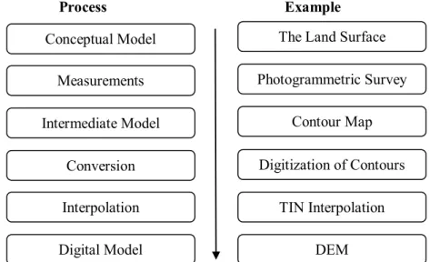
Figure 2.1 A flow chart showing the process of construction of a DEM through
the intermediary of a contour map. After Fisher and Tate (2006). 17 Figure 2.2 Examples of elevation data structure: (a) contour lines; (b) square grid;
and (c) triangular irregular network (TIN). Source: Wilson and Gallant (2000).
18
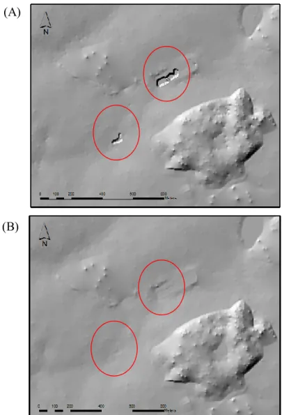
Figure 2.3 Digital elevation model and uncertainty (modified from Wilson, 2012) 26 Figure 2.4 Examples of spurious pits treatment using ArcGIS pit filling function
(A) snapshot of two pits from NEXTMap DTM shaded relief image (Wensum area) and (B) same area after pits filling treatment
38
Figure 2.5 Pit removal methods. The spurious pits are the two inner minima in
the graph (source: Peckham and Jordan, 2007) 39 Figure 2.6 Assignment of flow directions using the D8 model (modified from Li
et al. 2005)
42 Figure 2.7 Flow accumulation grid (A), flow accumulation with shading and (B),
and schematic of drainage network (C) (modified from Li et al. 2005). 43 Figure 2.8 Schematic illustration of relations between drainage area and local
slope depicting transition from hillslopes to valleys (Montgomery and Foufoula-Georgiou, 1993)
46
Figure 2.9 Two representations of the stream networks in the Blackwater sub-catchment of the River Wensum, reference network shown in blue and the derived stream network shown in red.
51
Figure 2.10 The epsilon band concept. The true position of the line (stream) will occur at some displacement from the measured position, between the two parallels of the epsilon band. Modified from Zhang and Goodchild (2002)
52
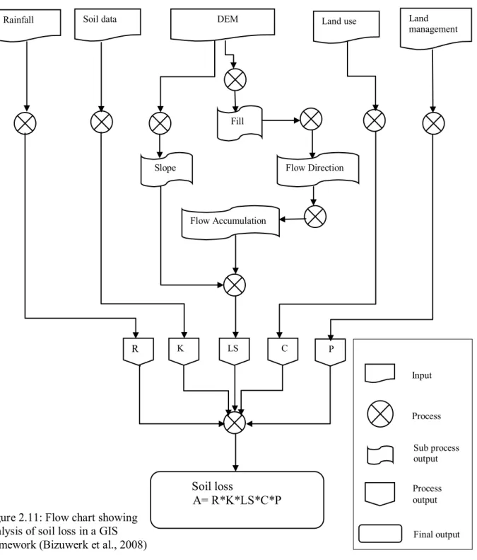
Figure 2.11 Flow chart showing analysis of soil loss in a GIS framework
(Bizuwerk et al., 2008) 60
Figure 2.12 SCIMAP model stages (SCIMAP project website:
www.scimap.org.uk) 64
Figure 3.1 Study area. 70
Figure 3.2 Land cover map 2007 for the study area 72
X
Figure 4.2 Locations of the cross-sectional lines 89
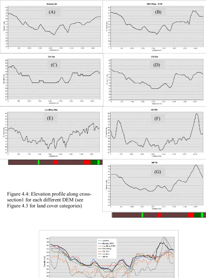
Figure 4.3 Location of cross-sectional line 1 overlaid on the land cover map. 90 Figure 4.4 Elevation profile along cross-section1 for each different DEM (see
Figure 4.3 for land cover categories) 92
Figure 4.5 Cross-section 1 showing difference between all the seven DEMs used
in this study. 92
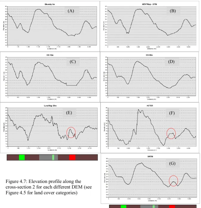
Figure 4.6 Location of the cross-sectional line 2 overlaid on the land cover map. 93 Figure 4.7 Elevation profile along the cross-section 2 for each different DEM
(see Figure 4.5 for land cover categories)
94 Figure 4.8 Cross-section 2 showing difference between all the seven DEMs used
in this study.
94 Figure 4.9 Examples of pit artifacts in an ASTER DEM normal image from the
Wensum area (A) and shown more clearly in shaded relief images (B & C).
96
Figure 4.10 Stripe effects (linear boundaries) in the LandMap dataset (A) and the associated abnormal elevation change is clear in the shaded relief images (B&C) and the elevation colour scheme image (D).
97
Figure 4.11 Land cover map 2007 (only three categories) overlaid on top of shaded relief image of the LandMap DTM form the River Wensum study area illustrating the effect of woodlands on the data.
98
Figure 4.12 Shaded relief map of Landform 10m DTM illustrating common problems associated with DTMs derived from contour data (triangular-shaped and stair-step) (A). Elevation profile indicates abnormal elevation change (2.3 meters) caused by unrealistic triangular-shaped relief (B).
99
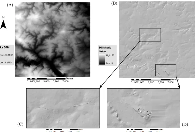
Figure 4.13 Examples of artifacts in the Bluesky DTM shaded-relief image (River Wensum area) that illustrate problems associated with DTMs derived from DSM data.
100
Figure 4.14 Examples of artifacts in the NEXTMap DTM shaded-relief image of Wensum area that illustrate problems associated with DTMs derived from DSM data.
101
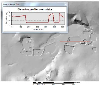
Figure 4.15 Elevation profile transect over a lake (Wensum River area) illustrating elevation differences between the lake and the surrounding terrain. 103 Figure 4.16 Examples of the spot heights used in this study as reference data (see
XI
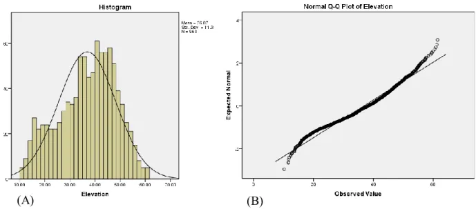
Figure 4.17 Distribution of the spot heights in the study area. 104 Figure 4.18 Histogram of the reference data with the normal curve superimposed
(A), and Normal Q – Q Plot for the reference data (B).
105 Figure 4.19 Cumulative probability distributions for K-S test. 108 Figure 4.20 Distribution of the differences comparing each DEM and the reference
data. 112
Figure 4.21 Cross-plots of reference heights versus corresponding heights from
each DEM (45 line would indicate perfect match). 113 Figure 5.1 Example of OS VectorMap™ water feature data for Blackwater study
area, (a) shows the breaks in the river segments (see red circles), and in (b) part of OS 1:1000 MasterMap illustrates that these breaks are indicative of road features intersecting the river, also in this figure the connected river segments are overlaid on the topographic map.
Source: Ordnance Survey.
121
Figure 5.2 Reference river network for the Wensum study area (OS MasterMap). 122 Figure 5.3 The stream networks extracted from each DEM using the selected
threshold value (0.625 km²). The reference river network is also illustrated.
126
Figure 5.4 The numbers of streams within each stream order from each DEM. 128 Figure 5.5 The stream networks extracted from each DEM using 1% of the
maximum flow accumulation value as the threshold (1.2 km²). The reference river network is also presented including the lakes layer.
130
Figure 5.6 Number of streams within each stream order from each DEM. 131 Figure 5.7 The differences between stream networks with 0.625 and 1.2 km²
thresholds.
132 Figure 5.8 Area-slope relationship with each data point being an average of 20
surrounding points (A), and cumulative area distribution (B) plots depicting the hillslope-to-valley transition (Hancock and Evans, 2006).
134
Figure 5.9 Area-slope relationship for Wensum study area. 135 Figure 5.10 Area-slope relationship for Wensum study area using Bluesky data
(arable and grass land cover categories only).
135 Figure 5.11 Area-aggregated slope relationship on semi-log scale separated into
regions based on scaling response. Vertical lines signify transitions between regions denoted by inflictions in the curve.
XII
Figure 5.12 Area-aggregated slope relationship in semi-log scale (A) and cumulative area distribution (B) for the entire study area using Bluesky data.
137
Figure 5.13 Area-aggregated slope relationship in semi-log scale (A) and cumulative area distribution (B) for the entire study area using NEXTMap data.
138
Figure 5.14 Stream networks extracted from Bluesky DTM in Blackwater sub-catchment at a contributing area of 25 pixels (0.000625 km²), transition between regions 1 and 2.
139
Figure 5.15 Stream networks extracted from Bluesky DTM in Blackwater sub-catchment at a contributing area of 200 pixels (0.005km²), transition between regions 2 and 3.
139
Figure 5.16 Stream networks extracted from Bluesky DTM in Blackwater sub-catchment at a contributing area of 50,000 pixels (1.25 km²), transition between regions 3 and 4.
140
Figure 5.17 Stream networks extracted from Bluesky DTM in Blackwater sub-catchment at a contributing area of 540,000 pixels (13.5 km²), transition between regions 4 and 5.
140
Figure 5.18 Streams obtained using 25pixels threshold are laid over the slope raster map. It is clear that low-order streams are a whole series of parallel lines going down the field when the variation in slope is in one direction.
142
Figure 5.19 Streams obtained using 25pixels threshold are laid over the aspect raster map.
142 Figure 5.20 The three locations investigated in the sub-catchment of the
Blackwater. The little arrows indicate the directions of the camera when photos were taken.
144
Figure 5.21 Landscape of location 1. Overland surface water accumulates to the bare part of this field as accurately captured by the DEM.
145 Figure 5.22 Landscape of location 2 (A). The arrow in image (B) indicates the
place at the edge of the field where the surface water accumulates before draining to the main stream just behind the long grass.
146
Figure 5.23 Landscape of location 3.
147
Figure 5.24 Comparison of the 50,000 pixels threshold delineated streams and the reference network.
148 Figure 5.25 Stream networks determined for the Blackwater sub-catchment at
contributing areas of 200, 50,000 and 540,000 pixels, 0.005, 1.25, 13.5 149
XIII km², respectively.
Figure 5.26 Area-aggregated slope plot for each DTM. The vertical dashed lines show the scaling regimes with respect to the four drainage area thresholds (25, 200, 50000 and 540000 pixels) that obtained using Bluesky DTM.
151
Figure 5.27 Area-local slope plot for the Brushy Creek basin (Alabama, USA). Four regions with different scaling response can be identified (Ijjasz-Vasquez and Bras, 1995).
154
Figure 5.28 Area-local slope plot for the Imnavait Creek Basin (Alaska, USA). Four regions with different scaling response can be identified (McNamara et al. 1999).
154
Figure 6.1 The number of streams within each stream order from each DEM (a) and the stream lengths (metre) within each stream order from each DEM (b) using the threshold value of 0.005 km² for the Blackwater sub-catchment.
164
Figure 6.2 The number of streams within each stream order from each DEM (a) and the stream lengths (metre) within each stream order from each DEM (b) using the threshold value of 1.25 km² for the Blackwater sub-catchment.
166
Figure 6.3 Monte Carlo simulation procedure used to produce stream probability maps from each DEM used in the study (modified from Lindsay, 2006).
168
Figure 6.4 ArcGIS Modelbuilder flowchart for the error propagation model used to produce a stream probability map for each DEM used in the study.
171 Figure 6.5 Results of the error propagation analysis for stream delineation from
(a) NEXTMap with RMSE of 2.032 m, (b) Bluesky with RMSE of 0.92 m, (c) OS50 with RMSE of 1.996 m and (d) SRTM with RMSE of 2.626 m. The model run for 100 iterations.
174
Figure 6.6 Example from OS50 data for the most probable stream created using
the cost path method. 176
Figure 6.7 Maps of the most probable stream network for each DEM. 177 Figure 6.8 Computation of horizontal RMSE between derived stream network
from NEXTMap data and the reference stream network for the Blackwater sub-catchment.
180
Figure 6.9 Illustration showing that the derived stream network was missing a stream segment compared to the reference network. Points on the reference segment (indicated with small arrow) in (a) were manually removed (b) before the calculation process to ensure one-to-one
XIV correspondence.
Figure 6.10 Illustration showing that all points on the reference polyline that were beyond the end of the derived polyline (a) were manually removed (b).
182 Figure 6.11 Illustration showing modified streams locations where the narrow
drainage channels are preserved through the woodland area, NEXTMap example from Blackwater sub-catchment.
184
Figure 6.12 Frequency distribution of the distance differences between each derived stream network and the reference network within 10m,20m, 30m, ..., and 230m.
185
Figure 6.13 Cumulative frequency of the distance differences between each
derived stream network and the reference network. 186 Figure 6.14 Reference network and NEXTMap stream network overlying a
NEXTMap hillshade model (right) and Bluesky stream network overlying a Bluesky hillshade model (left). Note the big flat area in the Bluesky image resulting from the pit filling algorithm during the process of filling a huge sink created by an artifact behaving as a dam.
187
Figure 6.15 Cumulative frequency of the distance differences between the most probable stream networks and the reference network.
189 Figure 6.16 Frequency distribution of the distance differences between the most
probable stream networks and the reference network within 10m ,20m, 30m, ..., and 210m.
190
Figure 6.17 The epsilon band concept. The true position of the line (stream) will occur at some displacement from the measured position, between the two parallels of the epsilon band.
191
Figure 6.18 A buffer of width 70m placed around the reference network, and the position of the NEXTMap derived stream network relative to the buffer. This illustration is shown as an example.
192
Figure 6.19 Illustrations of the portions of the NEXTMap derived stream network lying inside the buffer for width of (a) 5m (20.99 %), (b) 10m (35.78 %), (c) 20 m (65.09 %), (d) 30 m (79.58 %), (e) 40 m (88.84 %), (f) 50 m (93.71 %), (g) 60 m (97.18 %), (h) 70 m (98.97 %) and (i) the original NEXTMap streams (100 %).
192
Figure 6.20 An illustration of the percentage of each extracted stream network
lying within the buffer versus the buffer width. 194 Figure 6.21 Illustrations of the portions of each derived stream network lying
inside each buffer width. Line breaks depict sections of each stream network lying outside the buffer.
XV
Figure 6.22 An illustration of the percentage of each extracted most probable stream network lying within the buffer versus the buffer width.
199 Figure 7.1 In channel risk mapping for the Blackwater sub-catchment using OS
50m DEM, the accumulated risk weighted by the dilution potential. Areas in red show where there is more diffuse pollution risk than water to dilute the risk and green areas show where there is less risk.
213
Figure 7.2 Network index values for the Blackwater sub-catchment. The network index is used as representation of surface connectivity risk. Blue represents the highest potential connectivity and red the lowest.
215
Figure 7.3 Blackwater sub-catchment potential pattern of surface erosion. Red is the highest relative risk, blue is the lowest.
215 Figure 7.4 In channel risk mapping for the Blackwater sub-catchment, the
accumulated risk weighted by the dilution potential. Areas in red show where there is more diffuse pollution risk than water to dilute the risk and green areas show where there is a less risk.
217
Figure 7.5 In channel risk mapping, the accumulated risk weighted by the dilution potential (a) mini-catchment A and (b) mini-catchment B. Areas in red show where there is more diffuse pollution risk than water to dilute the risk and green areas show where there is less risk.
218
Figure 7.6 Soils map of the Blackwater sub-catchment indicating the different soil types.
226
Figure 7.7 K factor raster map. 227
Figure 7.8 Slope (%) (a) and LS-factor (b) from NEXTMap data. (c) and (d) from OS50 data. It is clear that LS-factor is strongly influenced by cell size. 229 Figure 7.9 C-factor raster map (5 x 5 m) for the farming year of 2011/12. 238 Figure 7.10 C-factor raster map (5 x 5 m) for the farming year of 2012/13.
239
Figure 7.11 P-factor raster map (5 x 5 m). 244
Figure 7.12 Soil erosion risk map for Blackwater sub-catchment. Farming year 2011/12 – NEXTMap.
243 Figure 7.13 Soil erosion risk map for Blackwater sub-catchment. Farming year of
2012/13 – NEXTMap. 248
Figure 7.14 Soil erosion risk map for Blackwater sub-catchment. Farming year
2011/12 – OS50. 251
Figure 7.15 Soil erosion risk map for Blackwater sub-catchment. Farming year
XVI
Figure 7.16 Soil erosion risk map for Blackwater sub-catchment. Farming year 2011/12 – NEXTMap 50-m
255 Figure 7.17 Sugar beet fields in mini-catchment A and B highlighted differently
for each season.
265 Figure 7.18 Impact of sugar beet harvesting on soil erosion. These photos were
taken from Wood Dalling field on 27 November 2012. The right photo highlights the large suspended sediment concentration coming from a tributary due to sugar beet harvesting upstream.
266
Figure 7.19 Turbidity mean values averaged for each four months. 268 Figure 7.20 Sediment load of the two mini-catchments (A and B) for each four
months.
269 Figure 7.21 Soil erosion risk maps for mini-catchment A, (a) normal Scenario, (b)
first level assessment of measures for soil erosion risk (Scenario one), by adopting different tillage practices, contour tillage (P =0.5) where sugar beet or potatoes occurred and strip tillage (P=0.37) for any other crop, (c) second level assessment of measures for soil erosion risk (Scenario two), by replacing any sugar beet, potatoes or maize crops with either wheat, barley or oilseed rape, according to the previous crop grown at the proposed field. Note: In scenario two, all fields were assumed to be cultivated with strip tillage.
276
Figure 7.22 Soil erosion risk maps for mini-catchment B, (a) normal Scenario, (b) first level assessment of measures for soil erosion risk (Scenario one), by adopting different tillage practices, contour tillage (P =0.5) where sugar beet or potatoes occurred and strip tillage (P=0.37) for any other crop, (c) second level assessment of measures for soil erosion risk (Scenario two), by replacing any sugar beet, potatoes or maize crops with either wheat, barley or oilseed rape, according to the previous crop grown at the proposed field. Note: In scenario two, all fields were assumed to be cultivated with strip tillage.
276
Figure 7.23 Areas occupied by each class of erosion severity (left Y axis) and their percentages from whole catchment area (right Y axis), according to the three scenarios adopted.
277
Figure 7.24 Soil erosion risk maps for mini-catchment A, (a) normal scenario, (b) first level assessment of measures for soil erosion risk (Scenario one), by adopting different tillage practices, contour tillage (P =0.5) where sugar beet or potatoes occurred and strip tillage (P=0.37) for any other crop, (c) second level assessment of measures for soil erosion risk (Scenario two), by replacing any sugar beet, potatoes or maize crops with either wheat, barley or oilseed rape, according to the previous crop grown at the proposed field. Note: In scenario two, all fields were
XVII assumed to be cultivated with strip tillage.
Figure 7.25 Soil erosion risk maps for mini-catchment B, (a) normal scenario, (b) first level assessment of measures for soil erosion risk (Scenario one), by adopting different tillage practices, contour tillage (P =0.5) where sugar beet or potatoes occurred and strip tillage (P=0.37) for any other crop, (c) second level assessment of measures for soil erosion risk (Scenario two), by replacing any sugar beet, potatoes or maize crops with either wheat, barley or oilseed rape, according to the previous crop grown at the proposed field. Note: In scenario two, all fields were assumed to be cultivated with strip tillage.
282
Figure 7.26 Areas occupied by each class of erosion severity (left y- axis) and their percentages from whole catchment area (right y-axis), according to the three scenarios adopted.
283
Figure 7.27 Blackwater sub-catchment models showing areas at high risk of erosion based on (a) SCIMAP and (b) RUSLE.
XVIII LIST OF TABLES
Table 1.1 Key characteristics of DEM different data sources. 5
Table 2.1 DEM derivatives and their application. 31
Table 4.1 Characteristics of DEMs used in this study. 85
Table 4.2 Elevation descriptive statistics. 86
Table 4.3 Slope descriptive statistics. 86
Table 4.4 Descriptive statistics for the reference data. 106
Table 4.5 K-S test statistics output table. 108
Table 4.6 Statistics of DEMs comparison with 963 spot heights (units are in metres).
110 Table 5.1 Flow accumulation threshold values for each different DEM. 124 Table 5.2 The numbers of streams within each stream order from each DEM. 127 Table 5.3 Flow accumulation threshold as a 1% of the maximum flow
accumulation value for each DTM.
128 Table 5.4 The numbers of streams within each stream order from each DEM. 131 Table 5.5 Comparison of total numbers of streams and highest stream order from
each DEM using 0.625km² (visual judgment) and 1.2km² (%1 of the maximum flow accumulation value) threshold values.
132
Table 5.6 The numbers of streams within each stream order from Bluesky DTM using the four threshold values obtained using method 3.
145 Table 5.7 The number of pixels from each DEM corresponding to each
contributing drainage area (thresholds) that were obtained from Bluesky.
152
Table 5.8 Streams order, numbers of streams and streams lengths obtained from BlueskyDTM using different threshold values.
153 Table 6.1 The number of streams, total stream lengths and the total catchment
area for the Blackwater sub-catchment from each DEM using the threshold value of 0.005 km².
162
XIX
order for the Blackwater sub-catchment from each DEM using the threshold value of 0.005 km².
Table 6.3 The number of streams, total stream lengths and the total catchment area for the Blackwater sub-catchment from each DEM using the threshold value of 1.25 km².
165
Table 6.4 The number of streams and the stream lengths within each stream order for the Blackwater sub-catchment from each DEM using the threshold value of 1.25 km².
166
Table 6.5 Minimum, maximum, mean, median, standard deviation and RMSE values for the distance differences between the derived stream networks and the reference network. The percentage of the distance differences that are equal or less than 10 and 20 metres is also reported. Results when 5 m spacing was used are reported inside the brackets.
182
Table 6.6 Minimum, maximum, mean, median, standard deviation and RMSE for the distance differences between the most probable stream networks and the reference network. The percentage of the distance differences that are equal or less than 10 and 20 metres is also reported.
188
Table 6.7 Results showing the length and percentage of each DEM extracted stream network for the Blackwater sub-catchment inside the buffer in terms of its width.
196
Table 6.8 Results showing the length and percentage of each DEM extracted most probable stream network for the sub-Blackwater sub-catchment inside the buffer in terms of its width.
200
Table 7.1 Default land cover risk weighting used in the SCIMAP framework. 211 Table 7.2 Numerical values from the SCIMAP final risk map and the water
quality data for mini-catchments A, B, C and D.
220
Table 7.3 Approximation R equations. 224
Table 7.4 Monthly precipitation records for Blackwater sub-catchment (mm). 224 Table 7.5 K factor values for different soil classes as used by USLE. 226
Table 7.6 M values for LS factor. 228
Table 7.7 Typical sowing and harvesting dates for a selection of crops grown in the UK.
233 Table 7.8 An example of three year crop rotations for some fields in the study
area.
XX
Table 7.9 Crop management factor (C-factor) for different land use/land cover categories cited in the literature.
236 Table 7.10 The median and the average of the C-factor values for each crop
reported in Table 7.9 above.
237 Table 7.11 C-factor values for main crop groups from Suri et al. (2002). 237
Table 7.12 P Factor Data. 240
Table 7.13 Assessed soil erosion intensities for Blackwater study area. Farming year 2011/12 – NEXTMap.
243 Table 7.14 The annual soil loss rates based on the land use for Blackwater study
area. Farming year 2011/12 – NEXTMap.
244 Table 7.15 Assessed soil erosion intensities for Blackwater study area. Farming
year 2012/13 – NEXTMap. 247
Table 7.16 The annual soil loss rates based on the land use for Blackwater study area. Farming year 2012/13 – NEXTMap.
248 Table 7.17 Estimated amount of soil eroded from the entire Blackwater
sub-catchment for the two seasons. 249
Table 7.18 Assessed soil erosion intensities. Farming year 2011/12 – OS50.
251 Table 7.19 The annual soil loss rates based on the land use. Farming year 2011/12
– OS50.
252 Table 7.20 Assessed soil erosion intensities. Farming year 2012/13 – OS50.
253 Table 7.21 The annual soil loss rate based on the land use. Farming year 2012/13
– OS50. 253
Table 7.22 Assessed soil erosion intensities. Farming year 2011/12 – NEXTMap 50-m
255 Table 7.23 The annual soil loss rates based on the land use. Farming year 2011/12
– NEXTMap 50-m
256 Table 7.24 Blackwater sub-catchment slope values for different resolutions. 258 Table 7.25 Blackwater sub-catchment LS values for different resolutions. 258 Table 7.26 Rates of soil erosion in terms of crop types for min-catchments A and
B in the Blackwater sub-catchment.
262 Table 7.27 Number of fields in terms of crop type in mini-catchments A and B for 265
XXI season 2011/12 and 2012/13.
Table 7.28 Descriptive statistics for turbidity measurements recorded at the outlet of sub-catchment A and B. the mean value is the average of each four months.
268
Table 7.29 Sediment load estimated according to turbidity measurements of
mini-catchments A and B. 269
Table 7.30 Descriptions of the different scenarios. 273
Table 7.31 Rates of soil erosion in mini-catchment A and B in terms of crop types based on the three scenarios.
278 Table 7.32 Rates of soil erosion in mini-catchments A and B in terms of crop
types based on the three scenarios.
XXII LIST OF ABBREVIATIONS
ASTER Advanced Spaceborne Thermal Emission and Reflection Radiometer CSA Critical Source Areas
CSF Catchment Sensitive Farming
CGIAR-CSI Consultative Group for International Agricultural Research Consortium for Spatial Information
DEFRA Department of the Environment, Food and Rural Affairs DEM Digital Elevation Model
DSM Digital Surface Model
DTC Demonstration Test Catchments DTM Digital Terrain Model
D8 Deterministic 8-Direction ERS European Radar Satellite
ERSDAC Earth Remote Sensing Data Analysis Centre FGDC Federal Geographic Data Committee
GDEM1 Global Digital Elevation Model Version 1 GDEM2 Global Digital Elevation Model Version 2 GIS Geographical Information Systems
HGCA Home Grown Cereals Authority IDB Internal Drainage Board
IFSAR Interferometric Synthetic Aperture Radar InSAR Interferometric Synthetic Aperture Radar JAXA Japan Aerospace Exploration Agency LCM 2007 Land Cover Map 2007
LiDAR Light Detection and Ranging
ME Mean Error
XXIII MFD Multiple Flow Direction
NDVI Normalised Difference Vegetation Index NSSDA National Standards for Spatial Data Accuracy NTU Nephelometric Turbidity Unit
OMAFRA Ontario Ministry of Agriculture Food and Rural Affairs
OS Ordnance Survey
OSGB36 Ordnance Survey Great Britain 1936 RBMP River Basin Management Planning RMSE Root Mean Square Error
RUSLE Revised Universal Soil Loss Equation SAC Special Area of Conservation
SD Standard Deviation
SCIMAP Sensitive Catchment Integrated Modelling and Analysis Platform SRTM Shuttle Radar Topography Mission
SSSI Sites of Special Scientific Interest SWAT Soil and Water Assessment Tool TIN Triangular Irregular Networks
USEPA US Environmental Protection Agency USGS United States Geological Survey USLE Universal Soil Loss Equation WEPP Water Erosion Prediction Program WFD Water Framework Directive WGS84 World Geodetic System 1984
XXIV ACKNOWLEDGEMENT
All gratitude to ALLAH for extending his grace, giving me the knowledge, passion and strength to complete this thesis.
I would like to express my sincerest gratitude to my main supervisor, Professor. Andrew Lovett, to whom I am particularly indebted for his trust, support, ideas, decisive guidance, and constant encouragement throughout the completion of this research. Without his support, it would have been impossible for me to complete this project. Sincere thanks also goes to my second supervisor, Professor. Kevin Hiscock, for his support and invaluable comments that increased the quality of outputs came out from the research work.
Special thanks are also due to the School of Environmental Science, UEA, and particularly to Dr. Faye Outram, Ms Gilla Sunnenberg and the Wensum Alliance who provided access to a number of datasets that were required in order to complete this project.
I also want to express deep and sincere gratitude to my father, brothers, sisters and friends who supported and encouraged me to complete this work.
Last, but not least, I would like to thank my wife, Mrs Samia, my son Abdulrahman and my two daughters Manar and Norah for their love, support and patience during my study. “Thank you for your love” is not enough to say to my wife, who put aside her dreams for fulfilling mine and only the days ahead of us can prove that her endless patience and constant encouragement were worth it.
1
Chapter 1
Introduction
1.1 Research context
The watershed, also termed catchment or river drainage basin, is a basic environmental unit where all surface water runoff flows downhill to a point on a stream (Gordon et al. 2004; Holden, 2014). It is an area defined naturally by surface water hydrology (Defra, 2013). A catchment is recognized as an appropriate scale for soil and water resources planning and management (Prato and Herath, 2007). Soil erosion and sediment transport, storage, and remobilization are controlled by hydrological and geomorphological processes which operate within the context of a catchment scale. Therefore, catchments are the natural scale for the assessment of soil erosion potential, and consequently water quality, since their shape and characteristics control the pathways and fluxes of water and sediment (Collins and Owens, 2006). It is now increasingly recognised that better coordinated action by all those who use water or influence land management is desirable at the catchment level. This, for instance, is central to the EU Water Framework Directive (WFD), a fundamental feature of which is the use of river catchments as reference units (Volk et al., 2010). The overall purpose of WFD is to achieve good ecological status for all European water bodies from 2015 onwards through the implementation of river basin management planning (RBMP) processes in all EU member states (Smith et al., 2014).
It is clear that catchments are an important functional entity for hydrological and landscape processes. Environmental processes are altered as landscape features are
2
manipulated and changed by human activities and the catchment is a natural scale to consider this aspect of the environment. In the UK this has been reflected in the promotion of the catchment-based approach to management and planning of the water environment with increasing support for local river trusts and research initiatives such as the Demonstration Test Catchments (DTC) programme (Defra, 2013; McGonigle et al., 2014).
The catchment area is an ideal unit to work with when looking at the land use management issues because everything is linked by water. What happens in one part of a catchment is likely to affect the remainder of the area. For example, a soil erosion problem in a farm in the upper headwaters may lead to diffuse pollution problems in lower parts of the catchment. The extent of such connections will depend on the topography, soil and geology of the catchment (Wu et al., 2007). Where the soil and geology are relatively impermeable the topography will be the key influence on the distribution and flux of water within the
catchment landscape. The digital representation of topography is termed a Digital Elevation Model (DEM). A DEM is therefore a core spatial dataset for catchment planning and management (McDougall et al., 2008).
1.1.1 The importance of DEMs
More generally, DEMs are one of the most fundamental types of spatial data used in Geographical Information Systems (GIS) (Li et al., 2005: Zhou et al., 2008). DEMs are a form of surface model widely employed in spatial modelling applications and for
environmental modelling in particular. They are essential for a wide range of applications in hydrology, geomorphology, ecology and other related fields (Maune, 2007; Li et al., 2005). These digital representations of topography can be used to perform numerous topographic analyses, such as calculations of slope, aspect, wetness index, topographic roughness and curvature among other topographic attributes (Lyon. 2003; Wilson, 2012; Wilson and Gallant, 2000). An extension of such topographic analysis is hydrographic feature extraction, which
3
includes delineation of stream profiles and catchments, and derivation of stream networks that represent catchment drainage (Liu and Zhang, 2011; Poggio and Soille, 2011; Gallego et al., 2010; Mantelli et al., 2011; Hengl et al., 2009; Joowon, 2011, Vianello et al., 2009). Many hydrological processes, such as soil erosion and sediment transport are strongly dependent on the landscape topography and linked to catchment as the spatial reference unit.
1.1.2 Sources of DEMs
Terrain data acquisition is the primary stage in digital elevation modelling. DEMs can be created from a number of different data sources as summarised in Table 1.1. Traditionally, these data have been obtained directly from field survey using surveying instruments such as a total station or GPS, digitising information from existing topographic maps, or
photogrammetric techniques (Li et al., 2005). These traditional methods can yield highly accurate digital elevation data, but they are also time consuming and labour intensive.
In the UK, Ordnance Survey (OS) DEMs have been a common sources of terrain data. The Ordnance Survey (OS) created 50 m Landform Panorama and 10 m Landform Profile digital terrain models (DTMs) from interpolation of mapped contour lines during the 1980s. These contour data were themselves captured from map series completed during the 1970s and 1980s using photogrammetric techniques (Ordnance Survey, 2010a and b).
During the past decade great progress has been made in more automated methods for DEM generation, particularly over larger regions and at the global scale. Remote sensing from both airborne and spaceborne sensors now provides an excellent source of worldwide DEM coverage (Wilson, 2012). This involves the use of optical satellite sensors, such as the Advanced Spaceborne Thermal Emission and Reflection Radiometer (ASTER) (ASTER Validation Team, 2009) and radar remote sensing sensors, such as the Shuttle Radar Topography Mission (SRTM) (Reuter et al., 2007).
4
The SRTM was a single pass interferometric synthetic aperture radar (IFSAR) mission conducted in February 2000 (Reuter et al. 2007). It was the first time that a global high-quality DEM was produced with a resolution of 1 arc-second (approx. 30 m) and 3-arc second (90 m), however of these two datasets only 90 m data are available globally, while the 30 m data are restricted to USA territory (Jarvis et al. 2008). The ASTER GDEM is derived from stereo processing of imagery from the ASTER instrument on the Terra satellite. Version 1 of the ASTER GDEM (a global 1 arc-second (30 m) elevation dataset) was released to the public in June 2009 (Hirt et al., 2010). An improved version of ASTER GDEM (ver. 2) was released in October 2011 (ASTER GDEM Validation Team, 2011). Currently there are two new satellite and sensor systems aiming to produce a global DEMs of even higher accuracy. These two missions are TanDEM-X which aims to produce a global 12 m resolution DEM based on IFSAR images, which will be available during 2014 (DLR, 2014), and the JAXA mission aiming to release a global 5 m resolution DEM (PRISM 5m DEM) during 2016 based on three optical systems on the ALOS satellite (JAXA, 2014).
Aerial photogrammetry and airborne radar interferometry have been used commercially to produce national coverage of high resolution DEMs. For example, the Bluesky 5m data were photogrammetrically interpolated from stereoscopic aerial photography and are available for England and Wales from the JISC Landmap service (Landmap 2011). Another example is the NEXTMap 5m data produced using an airborne IFSAR system for the USA, UK and some other countries within Europe and Asia by Intermap Technologies (Intermap, 2011). A further source of DEM information is LiDAR, which uses laser equipment on aircraft and can create very accurate and high spatial resolution representations of topography. At present, LiDAR is more of a local or regional data resource (e.g. for cities or coastal areas), but it is increasing in availability all the time (Goodchild, 2009; Robert et al., 2007). In response to all these advances in the production of DEMs, many studies have investigated the effects of
5
DEM data sources and resolutions on the creation of an accurate representation of the Earth’s surface and on derived topographic attributes (e.g. McDougall et al., 2008; Vaze et al., 2010).
1.1.3 Error and uncertainty in DEMs
Whatever the source of data all DEMs contain some inherent errors and these result in uncertainty regarding height values (Liu and Bian, 2008). This uncertainty in the DEM representation of the terrain surface propagates to the hydrological derivatives (e.g. slope, aspect) computed from the DEM (Wechsler, 2007: Wilson, 2012). Accuracy can affect the usefulness of a DEM dataset in hydrological applications, particularly in low relief areas (Chirico, 2004). For example, it can be important to assess the probability of an incorrect output from a hydrological flow model when a particular DEM is used (Darnell et al., 2010). It is common to admit that the accuracy of surface features will depend on the resolution and
Source Resolution (m) Accuracy Elevation/s
urface
Ground survey Variable but usually <5 m Very high vertical and horizontal Elevation
GPS Variable but usually <5 m Very high vertical and horizontal Elevation
Topo-map Depends on map scale and contour interval Very high vertical and horizontal Elevation
Ortho-photography <1 Very high vertical and horizontal Surface
LiDAR 1-3 0.15-1 m vertical, 1 m horizontal Surface
InSAR/IfSAR 2.5-5 1-2 m vertical, 2.5-10 m horizontal Surface
SRTM 90 16 m vertical, 20 m horizontal Surface
ASTER 30 7-50 m vertical, 7-50 m horizontal Surface
TanDEM-X 12 2-10 m vertical, ≤10 m horizontal Surface
JAXA 5 5 m vertical Surface
Table 1.1: Key characteristics of DEM different data sources.
Modified from Wilson, 2012; Nelson et al. (2010). TanDEM-X information were taken from Krieger et al., (2007), (DLR, 214) and JAXA DEM from (JAXA, 2014).
6
vertical accuracy of the DEM being used. However, some research (e.g. Hirt et al., 2010; Li and Wong, 2010; Zandbergen, 2006; Zhou and Liu, 2004) has demonstrated that coarser scale DEMs are sometimes more accurate in their representation of terrain surfaces, and that this can depend on the characteristics of the terrain itself and the nature of the analysis conducted (Wechsler, 2007).
From a practical point of view it is therefore important to regard the quality of a DEM as a combination of DEM accuracy and the suitability for a certain application (e.g. surface water flow path modelling) (Peckham and Jordan, 2007). Knowledge of the source data used to derive a DEM and its impact on hydrological derivatives can help when choosing an elevation dataset for a particular application. In other words, quantification of the accuracy associated with various DEMs (different sources and different resolutions) and subsequent hydrologic derivatives, drainage networks and catchment boundaries would assist other potential users in determining whether or not a specific dataset was appropriate for a particular application at a certain scale (i.e. fit for purpose).
As stated previously in Section 1.1.2, different sources, sensors, and formats with different characteristics like accuracy and spatial resolution have been developed to meet the rising demand for elevation data. Therefore, it is important that a user has an idea of how accurate a DEM that was created with a certain method is going to be used for a particular application (i.e. in catchment management) and the level of accuracy that can reasonably be expected. Numerous approaches have been developed to assess the accuracy of DEM
elevation values (Reuter et al., 2009; Wilson, 2012). This includes quantitative assessments of DEM accuracy as well as qualitative assessments of data usefulness (Carrara et al., 1997; Maune, 2007; Wilson and Gallant, 2000).
7
Many researchers have compared a set of heights extracted from the DEM with reference elevation values taken from a more accurate source of topographic data and then calculate the root mean square error of elevation (RMSE) to represent the differences between the estimated (DEM) and reference values (Hirt et al., 2010; Maune, 2007; Schumann et al., 2008; Wise, 2000; Wu et al., 2008). To fully address the DEM data for overall quality and suitability for an intended product, a qualitative assessment should also be performed. This may involve visually inspecting the spatial pattern of the DEM or its derivatives by means of a variety of rendering tools, such as shaded relief maps or other display techniques (Carrara et al., 1997; Maune, 2007).
1.1.4 Drainage network extraction from DEMs
In hydrology the accurate delineation of surface water drainage networks is a
prerequisite for investigation of many catchment-based natural resource management issues (Liu and Zhang, 2011) and is useful, for example, in distributed hydrological modelling, estimation of source areas, drainage density and downslope flow path length (Orlandini et al., 2011; Wilson, 2012). Surface water flow path is one of the most important hydrological parameters and investigation of the location of such networks within a watershed is vital. Ferrier and Jenkins (2010) argued that one of the key principles towards developing
sustainable management of catchments is to understand the natural processes occurring within a catchment and in particular, to determine the physical pathways of water movement
throughout the catchment landscape. The positive outcome of this will be seen in water management by helping land managers to choose the best management practices for maintaining water quality (Vieux, 2005).
Automated derivation of drainage networks and catchment boundaries from DEMs is a well-established technique used in terrain analysis (Vogt et al., 2003) and is primarily limited by landscape relief and DEM resolution (McMaster, 2002). The most commonly used
8
approach is based on the deployment of a model for surface water flow accumulation. As the flow of water is traced downhill from a point, flow accumulation is computed for all the downstream points through which the water flows such that an area threshold can be set whereby any points with an accumulation area higher than the threshold are defined as streams (Colombo et al., 2007). This threshold represents the minimum contributing area needed to form and maintain a drainage network. The choice of flow accumulation threshold influences the extracted drainage network (Lin et al., 2006; Orlandini et al., 2011). As the extraction of drainage networks in a catchment is the first step in the simulation of
hydrological processes (Paik, 2008), the choice of an appropriate threshold is vital (Colombo et al., 2007; McMaster, 2002; Orlandini et al., 2011; Wilson and Gallant, 2000).
Different DEMs with the same or different resolution will produce different realisations of stream networks and catchment boundaries. Uncertainty (error) exists in all spatial data (Zhang and Goodchild, 2002). However, the extent of differences in the derived stream networks and catchment boundaries will depend on the DEM resolution, technologies and methods used to collect the source data, the processing methods that are applied, and the complexity of the surface itself. Not surprisingly, the horizontal and vertical resolution of a DEM can have a significant influence on the accuracy of hydrologic delineations (i.e. drainage network) that are extracted from the DEM (Wilson, 2012). Therefore, the
comparison of stream networks and catchment boundaries derived from different DEMs is an important aspect of quality assessment and can indicate their suitability for a particular application (Charrier and Li, 2012; Hengl et al., 2009; Mantelli et al., 2011; Penas et al., 2011; Poggio and Soille, 2011). The horizontal accuracy of DEMs can be tested by
quantifying positional offset distances between the delineated drainage networks from each DEM and a higher accuracy reference stream network, if we assume that the reference data are the best available representation of this particular feature (Goodchild and Hunter, 1997).
9
The mean of these differences (RMSE) can be used to quantify horizontal offset error between the reference stream channel and the delineated drainage networks. In turn, these errors can be comparatively evaluated to determine which DEM best describes the relative terrain (Mantelli et al., 2011).
1.1.5 Soil erosion modelling
Within a watershed, surface runoff (sometimes termed overland flow) can play a very important role in soil erosion and transport of diffuse pollution (Vieux, 2005; Lane et al., 2006). Within a catchment, soil eroded from agricultural lands is one of the most obvious pollutants (Chapman et al., 2014) and may have other chemical particles (e.g. of phosphorus) associated with it (Haygarth et al., 2005). Hydrological pathways can exert a major control on where soil is eroded within a landscape and whether it is subsequently delivered to
watercourses (Ferrier and Jenkins, 2010; Reaney et al., 2011). Surface hydrological connectivity can be assessed through analysis of the potential pattern of soil moisture and saturation within the catchment (Lane et al., 2006). The spatial pattern of soil moisture throughout a catchment depends partly on its landscape topography (Wu et al., 2007). Therefore, DEMs are crucial surface representations in soil erosion modelling.
Digital elevation models have been widely used in a geographical information system (GIS) to extract the topographical and hydrological characteristics of a catchment in soil erosion and diffuse pollution studies (Datta and Schack-Kirchner, 2010; Shen et al., 2013). Estimation of soil erosion loss is often difficult due to the complex interplay of many factors, such as climate, land cover, soil type, topography, and human activities. Accurate estimation of soil erosion loss or evaluation of soil erosion risk at a catchment or river basin scale has become an urgent task (Owens and Collins, 2006). However, in many situations, land
managers and policy makers are more interested in the spatial distribution of soil erosion risk than in absolute values of soil erosion loss. To address this need the combined use of
10
geographical information system (GIS) and erosion models has been shown to be an effective approach in estimating the magnitude and distribution of soil erosion risk (Prasuhn et al., 2013). Studies have also been carried out to evaluate the effect of spatial resolution on the accuracy of soil erosion prediction (Cochrane and Flanagan, 2005; Lee and Lee, 2006; Molnar and Julien, 1998; Rojas et al., 2008; Wu et al., 2005; Zhang et al., 2008).
1.1.6 The role of GIS
Geographical information systems (GIS) are now considered as a key component of many environmental studies and their advantages for watershed studies have been recognised (Lovett and Appleton, 2008; Lyon, 2003). GIS are computer-based tools that facilitate
mapping and spatial analysis of the Earth's features and processes. One particularly important role of a GIS in catchment modelling is to provide an environment for the integration of spatial data at multiple scales collected from different sources (e.g. ground, air and space borne sensors) to create spatial datasets of catchment characteristics. Therefore, GIS layers describing topography, land use and land cover, soil types and, rainfall become model parameters or inputs in the simulation of hydrological processes (Vieux, 2005).
1.1.7 Summary
Catchments are increasingly recognised as important units for many types of
environmental management and planning. This is particularly true of the water environment, where local catchment-based approaches have become increasingly common in the UK. It is also clear that understanding of many key catchment processes depends on accurate
representations of the topography involved. As a consequence, it is important to evaluate the effect of using different DEMs in hydrological analysis and catchment management
applications. By doing so, it is hoped that this research will provide guidance to local
catchment managers and organisations such as river trusts about the best use of DEM datasets in developing catchment understanding and plans.
11
1.2 Aims and Objectives
1.2.1 Main aim
Given the above context the overall aim of this research is to understand accuracies and uncertainties associated with different digital elevation datasets derived from different sources and to explore the implications of their use in hydrological analysis and catchment
management applications. This will include the assessment of stream networks and catchment boundaries, as well as the implications for soil erosion and diffuse pollution modelling. The latter are particularly important in terms of the effective spatial targeting of catchment management activities.
1.2.2 Objectives
To achieve the general aim stated above, the specific objectives of this research are: 1. To evaluate the accuracy of different DEM datasets representing the same region
and surface type but derived from different sources.
2. To determine an appropriate threshold value (flow accumulation threshold) that can be used to accurately delineate channel networks in a study catchment. 3. To quantitatively compare the positional accuracy of drainage networks derived
from different DEMs.
4. To conduct an assessment of soil erosion and diffuse pollution risk in the study catchment using different DEMs. A particular focus of this investigation will be to identify the locations (or sub-catchments) of high risk soil erosion areas within the study catchment using RUSLE and SCIMAP modelling techniques.
12
1.3 Structure of the Thesis
This chapter has described the context of the thesis research and set out the general aim and objectives. Chapter 2 reviews the existing research literature with respect to Digital Elevation Models, drainage network extraction from DEMs and soil loss and diffuse pollution modelling. This leads to a refinement of the research objectives.
Chapter 3 briefly describes the study area (the River Wensum catchment). The descriptive of the elevation datasets (ASTER, SRTM, Landmap, Bluesky, OS Landform Panorama, OS Landform Profile and NEXTMap) as well as the quality assessment of all the elevation datasets used in the study are presented in Chapter 4. Quantitative and qualitative assessments of all DEMs are performed using several different approaches. Firstly, the accuracy of each DEMs is assessed using elevation and slope descriptive statistics and histograms, cross-sectional profiles, and analytical shading images (hillshade). Secondly, an analysis of DEM accuracy against a higher accuracy reference data set is undertaken. Finally, an assessment of whether or not these elevation datasets are of sufficient quality (fitness for purpose) for catchment management studies is made, and five elevation datasets out of seven are selected for further investigation.
Chapter 5 is devoted to the determination of an appropriate supporting area threshold to delineate an adequate channel network in the Blackwater sub-catchment using the selected DEMs from the previous chapter. Three approaches are examined; trial and error, 1% of the maximum flow accumulation value (a rule of thumb), and the area-slope relationship approach. Chapter 6 goes on to compare the extracted stream networks using two different methods. In the first, stream networks are extracted directly from the original DEMs; in the second, an error propagation method (Monte Carlo approach) is used to determine a
probabilistic estimation of the stream networks and then identify the most probable stream network. The second part of this chapter investigates the positional accuracy of the predicted
13
stream networks by comparing them with a higher accuracy reference drainage network using horizontal RMSE and different buffer zones.
Chapter 7 examines soil erosion and diffuse pollution issues within the study catchment using the SCIMAP and RUSLE modelling frameworks. Outputs from the SCIMAP diffuse pollution and fine sediment connectivity model are discussed in the first part of the chapter. The second part outlines the use of the empirical universal soil loss equation (RUSLE) to estimate potential soil loss from fields in the study catchment. Within a GIS environment the RUSLE is then applied to the study catchment for two different farming years using two different DEMs. Results from both SCIMAP and RUSLE are compared to each other and also are validated and compared against water quality data collected across the study catchment. The final chapter (Chapter 8) summarises the main findings of this study, considers the implications for catchment management and discusses future research priorities.
14
Chapter 2
Literature review
2.1 Introduction
Chapter 1 highlighted how a catchment-based approach has been promoted by a range of organisations and initiatives for effective management of water quality. These include the EU Water Framework Directive (WFD) (Benson et al., 2014), the US Environmental
Protection Agency (USEPA) in America (Ferrier and Jenkins, 2010) and the Demonstration Test Catchment (DTC) programme in the UK (McGonigle et al., 2014). The WFD aspires to achieve good ecological and good chemical status for all surface waters through successive six-year cycles of measures (initially 2009-15). A surface water is defined as of good
ecological status if there is only slight departure from the biological community that would be expected in conditions of minimal human impact (Kallis and Butler, 2001). It has also been recognised that the key principles towards developing sustainable catchments management are firstly to understand the hydrological processes occurring within the catchment, in particular, to determine the surface pathways of water movement across the catchment landscape. Secondly, to identify possible locations within the catchment landscape where nutrients and pollutants are generated (e.g. hotspots of soil erosion) and how they may be transported to the watercourses. It has been shown that catchment geomorphology and
15
provide a wealth of information regarding catchment geomorphology and hydrology (Martinez at al., 2010). Therefore, ensuring that a DEM dataset accurately represents catchment surface topography is critical to understanding the natural processes occurring throughout the catchment landscape, which in turn has an important bearing on water quality management. Hence, this chapter starts (Section 2.2) by providing insight into DEMs
themselves, their sources, structure, associated uncertainty, and their derived topographic parameters. This leads on to consideration of issues related to drainage network extraction and diffuse pollution modelling.
2.2 Digital Elevation Models (DEMs)
2.2.1 Concept and definition
Digital elevation data are samples of the Earth’s surface elevations stored and handled in a digital environment, which have been defined by many authors in many different ways. The simplest definition is the one by Burrough (1986) that the DEM is any digital
representation of the continuous variation of relief over space, or more briefly any digital representation of the terrain. Based on one of the most widespread definitions, the digital elevation model is a representation of the Earth’s surface excluding natural or artificial features (Peckham and Jordan, 2007). Also, a DEM is defined as a mathematical model of the Earth‘s surface that, at present, is the most powerful method of representing relief. Fisher and Tate (2006, p.468) have defined a DEM as “a set of elevation values which are recorded on a regular grid, most commonly in a square form, less frequently in a triangular or
rectangular form”. Three types of terrain model are commonly distinguished: digital elevation model (DEM), digital terrain model (DTM) and digital surface model (DSM) (Maune, 2007).