2017
Triangle counting in graph streams: Power of
multi-sampling
Neeraj Kavassery Parakkat
Iowa State UniversityFollow this and additional works at:
https://lib.dr.iastate.edu/etd
Part of the
Computer Sciences Commons
This Thesis is brought to you for free and open access by the Iowa State University Capstones, Theses and Dissertations at Iowa State University Digital Repository. It has been accepted for inclusion in Graduate Theses and Dissertations by an authorized administrator of Iowa State University Digital Repository. For more information, please [email protected].
Recommended Citation
Kavassery Parakkat, Neeraj, "Triangle counting in graph streams: Power of multi-sampling" (2017).Graduate Theses and Dissertations. 16152.
by
Neeraj Kavassery Parakkat
A thesis submitted to the graduate faculty
in partial fulfillment of the requirements for the degree of
MASTER OF SCIENCE
Major: Computer Science
Program of Study Committee: PavanKumar Aduri , Major Professor
Samik Basu David Fernandez Baca
The student author, whose presentation of the scholarship herein was approved by the program of study committee, is solely responsible for the content of this thesis. The Graduate College will ensure this thesis is globally accessible and will not permit alterations after a degree is conferred.
Iowa State University Ames, Iowa
2017
TABLE OF CONTENTS Page LIST OF TABLES . . . iv LIST OF FIGURES . . . v ACKNOWLEDGEMENTS . . . vi ABSTRACT . . . vii CHAPTER 1. INTRODUCTION . . . 1
1.1 The streaming model . . . 1
1.2 Contribution . . . 2
CHAPTER 2. REVIEW OF LITERATURE . . . 4
2.1 Non-Streaming algorithms . . . 4
2.2 Streaming algorithms . . . 4
CHAPTER 3. MULTI-SAMPLING ALGORITHMS . . . 6
3.1 Algorithm variations . . . 6
3.2 Edge-vertex multi-sampling (EVMS) . . . 6
3.3 Theoretical Preliminaries . . . 7 3.4 EVMS Algorithm . . . 8 3.4.1 Algorithm . . . 8 3.4.2 Theoretical Analysis . . . 9 3.4.3 Memory bounds . . . 15 3.4.4 Time Complexity . . . 16
3.5 EVMS - Reservoir sampling . . . 16
CHAPTER 4. EXPERIMENTAL EVALUATION . . . 18
4.1 Datasets used . . . 19
4.2 EVMS sampling . . . 20
4.2.1 EVMS vs EVSS algorithm . . . 21
4.2.2 EVMS vs Triest-Base algorithm . . . 22
4.2.3 EVMS vs Neighborhood Sampling . . . 23
4.2.4 EVMS vs Colorful triangle Counting . . . 23
CHAPTER 5. CONCLUSION AND FUTURE WORK . . . 29
LIST OF TABLES
Page
Memory functions for the various algorithms . . . 19
Properties of the various datasets considered for the experiments . . . 20
Results of the EVMS algorithm for various graphs . . . 25
EVMS vs EVSS sampling . . . 26
EVMS vs Triest Base . . . 27
EVMS vs Colorful triangle counting . . . 28 Table4.1 Table4.2 Table4.3 Table4.4 Table4.5 Table4.6
LIST OF FIGURES
Page
Construction of auxiliary graph from the sampled triangles . . . 13
Tm vsT ime for Triest-base, EVSS and EVMS algorithms . . . 22
Tm vsT ime for Triest-base and EVMS algorithms . . . 23
Tm vsT ime for Colorful Triangle and EVMS algorithms . . . 24
Figure 3.1
Figure4.1 Figure4.2 Figure4.3
ACKNOWLEDGEMENTS
I would like to take this opportunity to express my thanks to those who helped me with various aspects of conducting research and the writing of this thesis. First and foremost, Dr. Pavan Aduri for his guidance, patience and support throughout this research and the writing of this thesis. His insights and words of encouragement have often inspired me and renewed my hopes for completing my graduate education. I would also like to thank my committee members for their efforts in reviewing this work: Dr. Samik Basu and Dr. David Fernandez Baca.
ABSTRACT
Some of the well known streaming algorithms to estimate number of triangles in a graph stream work as follows: Sample a single triangle with high enough probability and repeat this basic step to obtain a global triangle count. For example, the algorithm due to Buriol et al.[6] uniformly at random picks a single vertex v and a single edge e and checks whether the two cross edges that connectvtoeappear in the stream. This basic sampling step is repeated multiple times to obtain an estimate for the global triangle count in the input graph stream.
This work, proposes a multi-sampling variant of this algorithm: In case of Buriol et al’s algo-rithm, instead of randomly choosing a single vertex and edge, randomly sample multiple vertices and multiple edgesand and collect cross edges that connect sampled vertices to the sampled edges. We provide a theoretical analysis of the algorithm and prove that this simple modification yields improves upon the known space and accuracy bounds. We experimentally show that the algorithm out performs several well known triangle counting streaming algorithms.
CHAPTER 1. INTRODUCTION
With the current scale of web based networks, it is often extremely difficult to calculate the ex-act charex-acteristic of graphs, the main reason being their humongous size which makes it inefficient to apply traditional algorithms. It is often sufficient to obtain an approximate estimation of these characteristic quantities. One such quantity is the number of triangles in the graph.
Triangle is the smallest non-trivial clique of a graph. Understanding coarser and finer properties of triangle structures in a network has found applications in various areas such as social network analysis, recommendation systems, spam and fraud detection, and understanding network struc-ture and evolution [29, 4, 8, 9, 20, 3, 7, 26]. For example, the frequently used notions oftransitivity coefficientandclustering coefficientcritically depend on the number of triangles present in a social network. Many of the applications involve estimating these co-coefficients. With the advent and presence of very large scale graphs such as online social networks and web graphs, the computa-tional complexity of computing the number of triangles of a graph has received a lot of attention. Since exact triangle computation is expensive on large scale graphs, considerable emphasis has been placed on designing algorithms that willestimate the number of triangles of a graph withprovable guaranteeson the quality of the estimation.
1.1 The streaming model
One of the practical and well accepted models of computation for large scale data analytics is that of data stream model. In this model the data items arrive as a stream and the goal is to compute a function over the entire stream. Often it is the case that the stream processor does not have enough resources to store the entire stream in its memory and perform an off-line
computation. Thus the processor can not access an individual item of the stream multiple times unless it is stored in the memory. This streaming model is applicable in scenarios where the volume and velocity of the data is huge. In the data stream model for graphs, the stream processor receives a stream (e1, e2,· · · , em) as input, where each ei is an edge of an underlying graph G = (V, E).
No assumption is made on the order in which the edges arrive. The goal is to compute a function of interest by observing the graph stream while using as little memory as possible. Due to the constraints on the memory, it is not possible to compute exact answers for most of the functions. Thus it is desirable to compute an approximate value of the underlying function.
1.2 Contribution
This thesis presents a new algorithm to estimate the number of triangles of a graph in the data stream model. The algorithms is based on the algorithm due to Buriolet al.[6]. A basic step in both the algorithms is that they sample a single triangle. Firstly, a high-level description of the triangle sampling procedures is provided. The streaming algorithm of Buriolet al. is as follows: Uniformly at random sample a vertexv and an edge ha, bi of the graph. The uniform sampling is done using the classical reservoir sampling technique. Once sampled, if the both cross edges ha, vi and hb, vi arrive then output 1 otherwise output 0. RunR independentof copies of this basic procedure and take the average output as an estimate for the the number of triangles. Let T denote the number of triangles of the graph and m, n denote the number of edges and vertices of the graph. They showed that ifRisO(mnT 12 log(1/δ)), then with probability at least (1−δ), the estimate is accurate within a relative error of , i.e, the estimate differs from correct value by at most T. From now we will refer to this algorithm asEdge-Vertex Single Sampling algorithm, EVSS algorithm for short.
The EVSS algorithm attempts to sample asingle triangle. Simply stated the main contribution in the thesis is the following: By Modifying the above procedures to sample multiple triangles we obtain better bounds on the memory and space used. Consider EVSS algorithm. Instead of picking
a single vertex and a single edge, pick multiple vertices and multiple edges , store the cross edges that connect the sampled vertices to the sampled edges, and count the number of triangles formed by sampled edges and cross edges and scale the number by an appropriate factor. Surprisingly, it is shown that this simple variant, not only outperforms the original algorithms but has better accuracy, space bound and runtimes compared to some state of the art triangle counting algorithms. A theoretical analysis of the algorithm is provided and the algorithm is experimentally evaluated. It is proved that the multi-sampling version of the EVSS algorithm uses O(m
√ ∆V √ T 1 log(∆V/δ))
memory to compute an (, δ)-approximation of number of triangles, here ∆V denotes the maximum
triangle degree of the graph (maximum number of triangles a vertex can participate in). The new variant has smaller factors in terms of—1 instead of 12. The algorithm is validated by performing an extensive set of experiments, where the proposed algorithm is compared to a few other well known algorithms. We empirically show that the new algorithms performs better than several other triangle counting streaming algorithms from the literature [23, 18, 19, 6]. The experiments show that even on very large graphs such as Orkut (containing more than 100 million edges), the estimates produced by our algorithm have very high accuracy (> 99%) while storing only 2% of the edges. Impressively, the run time is less than a minute.
CHAPTER 2. REVIEW OF LITERATURE
2.1 Non-Streaming algorithms
A naive method to count triangles is to consider all triplets in a graph and verify if they form a triangle. This takes O(n3) time, where n is the number of vertices of the graph. The algorithm proposed by Alon et al. [1] reduces the triangle counting problem into a matrix multiplication problem which runs in O(m1.4). Other simple counting algorithms are node and edge iterator algorithms. The node iterator counts for each node, the number of triangles contained in it. The edge iterator in turn counts the number of common neighbors that the vertices of each edge have. Though a lot of minor improvements have been suggested using special data structures, hashing and sorting techniques these algorithms run inO(mn) time with worst case run time ofO(n3). The above algorithms are suitable for smaller graphs, but are practically in-feasible to work on larger real time graphs.
2.2 Streaming algorithms
There has been an extensive body of research on the problem of exact and approximate tri-angle counts in various computational models [21, 25, 26, 27, 28, 24, 18, 14]. Here we restrict our attention to the prior in the data stream model. Bar-Yosseff et al. were the first to for-mally study the problem of triangle counting the data stream model [2]. They reduced the triangle counting problem on graphs to estimating zeroth and second frequency moments over numeric data.
Much of the latter work is is based on various sampling strategies in the sense that they attempt to sample a sub-graph of the original graph [17, 13, 5, 22, 11, 10, 12, 6, 19, 16, 23]. In the algorithm defined by R. Pagh et al[18], each vertex of the graph is colored with N = 1p colors randomly, the triangles having the same colored vertex are then counted. They claim that when
p≥max(δlognt ,
q
logn
t ), the triangle estimate is concentrated around its expectation. The work of
Buriolet al.[6], randomly picks a vertex and an edge and looks for the two cross edges that connect the sampled vertex and the sampled edge, and this process is repeated. The work [19], randomly picks an edge e1 and a random neighbor e2 and looks for a cross edge that connects e1 with e2.
Both these works use reservoir sampling to randomly picks vertices/edges. The work of Lim and Kang [16] uses a fixed probability to sample the edges (as opposed to reservoir sampling). They fix a parameterpand pick each edge with probabilitypand count the number of triangles formed by the sampled sub-graph. The recent work of Stefaniet al.[23] uses reservoir sampling to sample multiple edges and counts the number of triangles in the sampled-subgraph. Their algorithm also handles dynamic streams (where edges can be deleted) and can be used to obtain local-triangle counts. The memory used by these algorithms depend on various graph parameters such as number of vertices (n), number of edges (m), total number of triangles (T), maximum-degree (∆), maximum number of triangles an vertex participates (∆V) etc. We describe the EVSS sampling strategy in Algorithm
1from Buriol et al [6] as our multi-sampling algorithm is built on it’s base sampling strategy. This algorithm is repeated ∈12 times and the average is returned to get a triangle estimate.
Input:Edge StreamE
Initialize:i= 1, β= 0;
for ∀e=hu, wifrom edge streamEdo ifcoin(1
i) == head then
a←u;b←w;
v←vertex uniformly chosen fromV\{a, b}
x←f alse;y←f alse end if e == (a,v)then x←true end if e == (b,v)then y←true end i←i+ 1 end
if x←trueandy←truethen
β= 1 end returnβ;
CHAPTER 3. MULTI-SAMPLING ALGORITHMS
This section describes the EVMS algorithm proposed as part of the thesis. The algorithms is an extension to Buriolet al.[6] inspired by the multi sampling approach used by Stefaniet al.[23].
3.1 Algorithm variations
The EVMS algorithm in turn has two variations based on the sampling approach used. The sampling of edges and vertices can be done based on a fixed probability p, 0 < p < 1 or based on the reservoir sampling approach. One main difference between the two is the certainty of the sample size after the sampling process. In the reservoir sampling approach, the size of the sample is fixed whereas the sample size using the fixed sampling greatly depends on the value of p. The reservoir sampling works as follows: Let’s assume we have a graph stream where edge ei arrives
at time i. We need to maintain a reservoir R of size M. We sample the edge ei if|R|< M else
we sample ei by randomly replacing an element from R with probability Mi . Another variation in
the algorithms is the number of passes (multi-pass or single-pass) made on the graph stream. The thesis makes extensive theoretical and experimental analysis only on the single pass, fixed sampling version.
3.2 Edge-vertex multi-sampling (EVMS)
Before the algorithm is presented, we provide an intuitive reasoning behind as why multi-sampling is a better strategy. Consider a two trianglet1 ={a, b, c} and t2 ={a, d, e} that share a
vertexa. Assume that the order in which the edge appear in the stream isbc, ab, ca, ad, ae, de. The EVSS algorithm samples t1 if vertex ais sampled and the edge abis sampled which happens with
need to be repeated twice and thus probability of sampling both the triangles in 1/(mn)2. Suppose that we sample a single vertex and two edges (and look for cross edges), what is the probability that both t1 and t2 are sampled? This happens if the sampled vertex isa and the sampled edges
arebc and ad. This probability is proportional to 1/m2nwhich is higher than 1/(mn)2. Thus the second strategy has a better chance of entangled triangle (triangles that share a vertex/edge) than the first strategy. This is the rationale behind the multi-sampling algorithm.
Our algorithm works as follows: We fix two sampling probabilities pv and pe. For simplicity,
we assume that the vertex set V is known in advance. Later, we discuss how this assumption can be removed. We place each v ∈ V into a set Sv with probability pv. We then process the graph
stream—when an edge earrives place it in a set Se with probabilitype. In addition, if econnects
a vertex from Sv to an edge from Re, then we place ein a set Be. We call the edges from Re as
red edges and edges from Be as black edges. Note that an edge can be both red edge and black
edge.Let us denote the time at which an edgehu, vi appears in the stream asthu,vi. We count only the sampled triangles such that each triangle has exactly two black edges and a red edge, and the two black edges appear after the red edge in the stream. We scale this count with an appropriate factor to get a global estimate.
The reason we check for triangles in which black edges arrive after the red edges is, if we sample edges in the stream in order of arrivalha, bi as red,hb, dias black and hb, ci as red while the vertex
dis a sampled vertex, the edgehc, di can be sampled as a black edge afterwards. Then the triangle hb, c, dishould be counted as a sampled triangle. But we are not counting such triangles.
3.3 Theoretical Preliminaries
This section presents certain results used later in the theoretical analysis of the algorithms. Definition 3.3.1. Random Variable: A random variableX is a function from a sample space Ω,
Definition 3.3.2. Expectation of a random variable is defined as
E[X] =X
α
P r(X=α)α
Lemma 3.3.1. Chebyshev’s Inequality: Let X be a random variable. Then,
P r[|X−E(X)| ≥δ]≤ V ar(X)
δ2
Lemma 3.3.2. Chernoff Inequality: Let X1, X2...., Xm be independent random variables that take
values between 0 and 1. Let E(X1) =E(X2) =...= E(Xm) =p. Let X = X1+X2+...+Xm,
then P r[X/m−p ≥pδ]≤2e −δ2mp 2
Lemma 3.3.3. Hajnal-Szemer´edi Theorem: Every graph with n vertices and maximum vertex
degree at most k is k + 1 colorable with all color classes of size at least kn+1.
3.4 EVMS Algorithm
3.4.1 Algorithm
As mentioned above, in the fixed sampling approach, the vertices and edges are sampled with a fixed probability. Let us denote these probabilities aspv andperespectively. LetGbe input graph
with V as the vertex set and E as the edge stream of the graph G. Let Sv denote the sampled
vertex set, the set of all sampled triangles -Y, the set of all red edges -Re, and the set of all black
edges -Be. The algorithm can be implemented as a multi-pass algorithm, where initially we sample
vertices with probability pv, in the first pass we sample edges with probability pe. On the second
pass, we check if each edge can be sampled as black edge. This approach can be slow if the graph is too large or in real-world scenarios where it is often not practical to read the stream multiple times. The two passes can be easily combined to a single pass with a slight modification to the algorithm involving time stamps of the edges. The passes are combined such that every edge in the stream is considered to be sampled as a red edge as well as a black edge. A formal description of the EVMS algorithm can be found in Algorithm2. Here,Y is a random variable that denotes the
number of triangles sampled by the algorithm. The algorithm outputs p|Y|
vpe whose expected value is the number of triangles in the entire graph.
Input: Edge StreamE, vertex setV, pv, pe
Initialize: Sv=∅,Y =∅,Re=∅,Be=∅;
for everyv∈V do
if coin(pv) == head then Sv←Sv∪ {v}
end end
for ∀ei=ha, bifrom edge streamE do
if coin(pe) == head then Re←Re∪ {e}
end
if (a∈Sv andRehas an edge with vertex b) OR (b∈Sv andRe has an edge with vertex a)then Be←Be∪ {ei}
end
for every(ej, ek),ej∈Re,ek ∈Be such that (tej < tek)and(tej < te)andhe, ej, ekiforms a triangle do
Y ←Y ∪ hei, ej, eki
end end
Output: τ=|Y|/(pvpe)
Algorithm 2:EVMS - Fixed sampling
3.4.2 Theoretical Analysis
Let τ(G) be set of all triangles in graph G, and |τ(G)|=T. Lemma 3.4.1. Let t∈τ(G). The probability that t is sampled is,
P r[t∈Y] =pvpe
Proof. A triangle, ha, b, ci is sampled when one of its vertex and its opposite edge is sampled as a red edge. Since every vertex and edge is sampled with a fixed probability, pv and pe respectively,
and the two events are independent, the probability that a triangle , t ∈ τ(G) gets sampled is
To estimate the number of triangles, we consider the algorithm’s output into a random variable such that the expectation of the random variable gives the triangle estimate.
Lemma 3.4.2. The algorithm EVMS-fixed-sampling outputs τ whose expectation is the number of
triangles in the graphG.
Proof. Let us define a random variable X, which denotes the number of triangles sampled by the algorithm. Let us calculate the E[X]. To calculate E[X], we split the random variable X into smaller random variablesXi such that X=PXi,1≤i≤T. We define,
Xi = 1, if the ith triangle of the graph gets sampled
= 0, else
E[Xi] = P r[Xi= 1].1 +P r[Xi= 0].0
= pvpe
Since Xi is a 0,1 random variable, |Y|= T P i=1 Xi E[τ] = E[ T P i=1 Xi pvpe ] = 1 pvpe T X i=1 E[Xi] = T
Lemma 3.4.3. The EVMS algorithm returns a triangle estimate τ, such that
V ar[τ]≤ T pe ( 1 pv + 3∆VT) .
Proof. V ar[τ] = V ar[ 1 pvpe T X i=1 Xi] = 1 pv2pe2 T X i=1 T X j=1 Cov[Xi, Xj] = 1 pv2pe2 ( T X i=1 V ar(Xi) + T X i=1 T X i=1 i6=j Cov[Xi, Xj])
From the expression for Variance, V ar[Xi] =pvpe−pv2pe2. If trianglesiand j do not share a
vertex then Cov[Xi, Xj] = 0. Trianglesiand j can be dependent when they share the red edge or
the sampled vertex. If they share a vertex, Cov[Xi, Xj] =pepv2−pv2pe2.
Let us calculate an upper bound for
T P i=1 T P i=1 i6=j
Cov[Xi, Xj]. IfTv is the number of triangles incident
on vertex v, then, T X i=1 T X i=1 i6=j Cov[Xi, Xj] = T X i=1 T X i=1 i6=j (pepv2−pv2pe2) ≤ T X i=1 T X i=1 i6=j (pepv2) ≤ pepv2 X v∈G Tv2 ≤ pepv2 X v∈G Tv∆V ≤ pepv2∆V X v∈G Tv ≤ 3pepv2∆VT
Hence we have, V ar[τ] ≤ 1 pv2pe2 ( T X i=1 (pvpe−pv2pe2) + 3pepv2∆VT) ≤ 1 pv2pe2 ( T X i=1 (pvpe) + 3pepv2∆VT) = 1 pv2pe2 (T(pvpe) + 3pepv2∆VT) V ar[τ] ≤ T pe ( 1 pv + 3∆VT)
Theorem 3.4.4. Concentration using Chebyshev’s inequality: For any, δ∈(0,1), andpv =pe=
q, the EVMS fixed sampling algorithm returns a triangle estimate τ such that when
q ≥ −3∆V + q q∆2V + 42δ 2δ2 P r[|τ −T| ≥T]≤δ
Proof. The proof follows by simple application of Chebyshev’s inequality using the variance ob-tained from Lemma3.4.3. Recall that the output of the algorithm is X
pepv . P r[|pX epv −T| ≥T]≤ T pvpe(1+3P∆V) p2 vp2e2T2 ≤δ
For simplicity, if set pv =pe =q, after solving this inequality we get q ≥
−3∆V +
q
q∆2V + 42δ
2δ2 .
Thus the above algorithm outputs (, δ) approximation if pv = pe = q and the above inequality
holds.
Theorem 3.4.5. For any , δ ∈ (0,1), the EVMS fixed sampling algorithm returns a triangle
estimate τ such that when
pepv ≥ 2 2 3∆V + 1 T ln( 2(3∆V + 1) δ ) P r[|τ−T| ≤T]>1−δ
Proof. We can use Chernoff bounds to find the concentration bounds for the random variable X, since it can be split into smaller random variables with equal expectation. But one cavaet to ap-ply Chernoff bounds is that the random variables need to be independent. In this case, random variables, Xi and Xj are not independent when the triangles they represent share a vertex. One
way to deal with this is to group the triangles into groups, such that no triangle in a group share a vertex. Hence all random variables within a group are independent, enabling us to apply Chernoff bounds on each of these group. But how do we know how many such groups exist ?
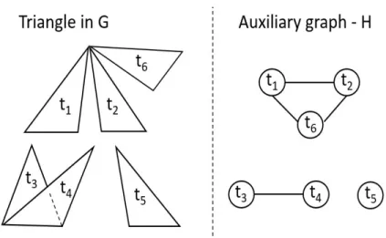
One way to find a lower bound on the number of groups is to build an auxiliary graph H and apply Hajanal-Szem´eredi therorem on the graphH. We buildH, so that for every triangle inτ(G), we have a corresponding vertex inH. An example of this construction is shown in Figure3.1. There is an edge between any two vertices in H if, the corresponding triangles in τ(G) share a vertex. Let the maximum number of triangles shared by a vertex in τ(G) be ∆V. By Hajanal-Szem´eredi
theorem,H can be properly colored with at most 3∆V + 1 colors, with atleast k= 3∆|τ(VG+1)| vertices
in each color.
Figure 3.1: Construction of auxiliary graph from the sampled triangles
Let us number each of the triangles inτ(G) by a arbitrary numberi, so that the random variable
be the set of random variables Xi, such that the nodeiinH has colorc. The random variables in
Yc are independent. Also it is to be noted that
P ∀c [ P Xi inYc Xi] = P ∀Xi andP ∀c k=T. Applying Chernoff bounds to the color set c, we have,
P r[| P Xi∈c Xi k −pepv| ≥pepv]≤2e −2kpepv 2 P r[| P Xi∈c Xi pepv −k| ≥k]≤2e− 2kpepv 2
The above equation shows the probability bound for a single color class. Hence, the probability that at least one of the class has P r[|
P
Xi∈c Xi
k −pepv|] ≥ pepv can be obtained by union over all
color sets. Let us denote this byδ.
X ∀c P r[| P Xi∈c Xi k −pepv| ≥pepv]≤ X ∀c 2e− 2kpepv 2 P r[| P ∀c P Xi∈c Xi pepv −T| ≥T]≤(3∆V + 1)2e −2kpepv 2 P r[| P Xi pepv −T| ≥T]≤(3∆V + 1)2e −2kpepv 2 P r[|τ −T| ≥T]≤(3∆V + 1)2e −2kpepv 2 P r[|τ −T| ≥T]≤δ Therefore, e− 2kpepv 2 ≤ δ 2(3∆V + 1) pepv ≥ 2 2 3∆V + 1 T ln( 2(3∆V + 1) δ )' ∆V 2Tln ∆V δ
From the above expression, we infer that when pepv ≥ 22
3∆V+1 T ln(
2(3∆V+1)
δ ), the EVMS fixed
3.4.3 Memory bounds
We now analyze the memory used by the algorithm. The memory used for this algorithm consists of the memory used to store the black and red edges. The expected number of red edges in total is pem. We can compute the expected number of black edges as follows: Letabbe an edge
of the graph. This becomes a black edge ifais inSv and an edge incident onb is sampled as a red
edge. The other case is when b is in Sv and an edge incident on a was is sampled as a red edge .
Let’s look at the former case. The vertexa∈Sv with probabilitypv. Letdbe the number of edges
that are incident on vertexband arrive before edgeab. Probability that at least one of these edges being a red edge is (1−(1−pe)d). Thusabbecomes black edge with probability (1−(1−pe)d)pv. In
general letd(e) denote the number of edges that arrive beforeeand is incident one. The expected number of black edges is at most
X e∈G [1−(1−pe)d(e)]pv =pv X e∈G 1−X e∈G (1−pe)d(e) =pv(m− X e∈G (1−pe)d(e))≤mpv
So the expected number of red and black edges is bounded bym(pe+pv). Subject to the constraint
from Theorem 3.4.5, pepv ≥ ∆2VTlog
∆V
δ the quantity pe +pv is minimized when pv = pe equals
q
∆V 2Tlog
∆V
δ . Thus the expected number of edges stored by the algorithm is O(mpe) and the
expected number of vertices stored is O(npe) which is O(mpe). Putting together we obtain the
Theorem 3.4.6. There is a streaming algorithm that computes (, δ)-approximation of number of
triangles in a graph by using expected space O(mp) where p equals q ∆V T 1 q log∆V δ . 3.4.4 Time Complexity
The running time of the algorithm depends only on the step that computes the exact count of the triangles from the vertex and edge samples. We use the edge iterator algorithm to find the exact count. The Edge Iterator algorithm computes for each edge the number of triangles it a part of. It does this by find the common neighbors of its end vertices. The time complexity of this algorithm isO( P
v∈Sv
d2
v).
3.5 EVMS - Reservoir sampling
3.5.1 Algorithm
The thesis gives a description of the reservoir sampling version of the algorithm, but does not discuss the theoretical and experimental analysis. In the reservoir sampling version of the EVMS algorithm, the vertices and red edges are sampled using a reservoir of fixed size. Let us denote the vertex reservoir memory as N and edge reservoir memory as M. Let n and m be the total number of vertices and edges respectively in the original graph. Let V = {vi,1 ≤ i ≤ n} and
E ={ei,1≤i≤m} be the vertex set and edge stream respectively. The formal description of the
Input: Edge StreamE, vertex setV, pv, pe Initialize: Sv=∅,Y =∅,Re=∅,Be=∅; for everyvi∈V do if |Sv|< N then Sv←Sv∪ {vi}; end
else if coin(Mi ) == head then
t←random vertex fromSv ; Sv←Sv\ {t};
Sv←Sv∪ {vi};
end end
for ∀ei=ha, bi from edge streamE do
if |Re|< M then Re←Re∪ {ei} ;
end
else if coin(Ni) == head then
x←random vertex from Re; Re←Re\ {x} ;
Re←Re∪ {ei} ;
end
if (a∈Sv andRehas an edge with vertex b) OR (b∈Sv andRehas an edge with vertex a) then Be←Be∪ {ei} ;
end
for every(ej, ek),ej∈Re,ek ∈Be such that(tej < tek)and(tej < tei)andhei, ej, eki forms a triangle do Y ←Y ∪ hei, ej, eki end end Output: |Y|mn M N
CHAPTER 4. EXPERIMENTAL EVALUATION
The experiments were performed to analyze the memory, accuracy, and speed of both the algo-rithms. The aim is to verify, for a given value of pv and pe the theoretical bounds hold true. We
also analyze how the parameters like maximum triangle degree, number of edges and transitivity co-efficient of the graph affect the accuracy of the algorithms. We run the algorithms with the probabilities set to 0.01,0.05,0.1,0.15 and 0.2. Hence for each graph, we have 25 possible experi-ments.
Experiments were conducted on several graphs from the Stanford Large Network Dataset Col-lection [15]. The implementation was done in Java 8, and run on a PC with Core i7 2.5 Ghz, 16GB RAM with Windows 10 operating system. The experiments were run on insertion only streams, where each edge is a new edge with no repetitions. The datasets were chosen in such a way that they have varying topologies. The graphs have varying densities ranging from around 900,000 edges (Amazon) to more than 100,000,000 edges (Orkut). The graph was pre-processed so that the vertices are numbered form 0 ton−1, wherenis the total number of vertices of the graph. In the implementations, the graph is represented as an adjacency list with a map of all the vertices and corresponding values as the list of all neighbors of that vertex.
The performance of the proposed algorithms were compared against EVSS algorithm from Bu-riol et al’s [6], Triest-Base [23], neighborhood sampling algorithm [19], and colorful sampling algorithm due to Pagh and Tsourakakis [18]. The rational for this choice of algorithms is as fol-lows: Naturally, we would like to compare EVMS and NMS against their counter parts. Since, Triest-Base [23], the authors experimentally showed that Triest-Base algorithm outperforms sev-eral other algorithms from the literature, we chose Triest-Base algorithm. We chose the colorful
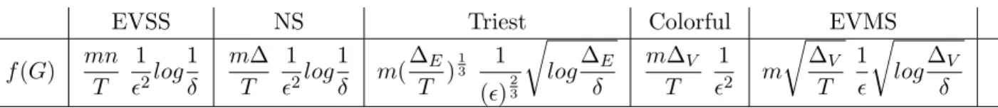
Table 4.1: Memory functions for the various algorithms
EVSS NS Triest Colorful EVMS
f(G) mn T 1 2log 1 δ m∆ T 1 2log 1 δ m( ∆E T ) 1 3 1 ()23 r log∆E δ m∆V T 1 2 m r ∆V T 1 r log∆V δ
triangle counting algorithm because as far as our knowledge its performance on graph streams has not been tested before. The theoretical memory bounds can be expressed as a function of the different parameters of the graph like number of vertices, edges and actual triangle count. Let us denote this as f(G). The f(G) for all the above algorithms are show in Table 4.1
All the above algorithms were implemented in java. The implementation is available at https:
//github.com/kpneeraj/triangle counting. The experiments were first run on the EVMS-fixed sampling algorithm with different values for pv and pe. To get a fair comparison, the other
algo-rithms were run using the total memory, Tm used by the both the algorithms. The total memory
is the sum of the red and black edges for the EVMS algorithm.
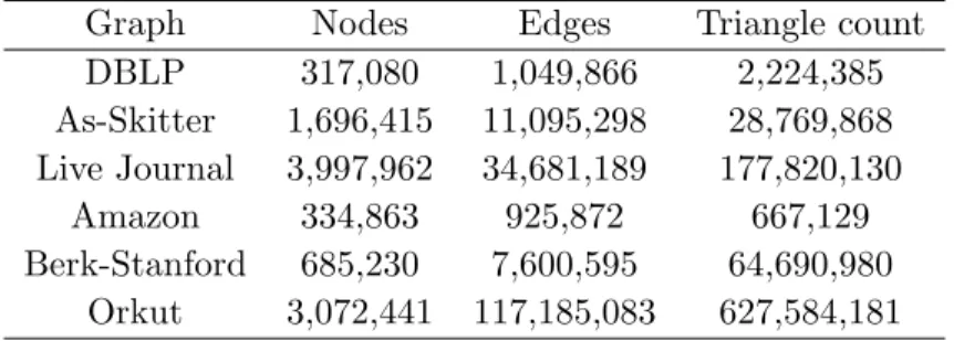
4.1 Datasets used
The following datasets [15] were used whose vertex and edge counts are shown in Table4.2. DBLP Collaboration network : A co-authorship network of computer science bibliography
where two authors are connected if they publish at least one paper together. Authors who pub-lished to a certain journal or conference form a community.
Skitter : An Internet topology graph from trace routes run daily in 2005 from several scattered
sources to million destinations.
Live-journal: A friendship graph of a free on-line blogging community where users declare
friend-ship among each other. Users are vertices and the presence of a edge represent friendfriend-ship between two users.
Amazon co-purchasing network: It is a graph built by collecting items that were purchased
Table 4.2: Properties of the various datasets considered for the experiments
Graph Nodes Edges Triangle count
DBLP 317,080 1,049,866 2,224,385 As-Skitter 1,696,415 11,095,298 28,769,868 Live Journal 3,997,962 34,681,189 177,820,130 Amazon 334,863 925,872 667,129 Berk-Stanford 685,230 7,600,595 64,690,980 Orkut 3,072,441 117,185,083 627,584,181
represent the fact that the products are frequently purchased with each other.
Berkeley-Stanford web graph : Nodes represent pages from berekely.edu and stanford.edu
do-mains and edges represent hyperlinks between them. The graph was initially directed, which was converted to undirected by removing redundant edges that represent direction.
Orkut web graph: A friendship graph of the Orkut social network where each vertex is a person
and each edge represents friendship between two people.
4.2 EVMS sampling
Since the vertices are numbered from 0 ton−1, the first step of vertex sampling is replaced by sampling integers from 0 ton−1 with probabilitypv. The implementation of the EVMS algorithm
maintains two adjacency lists one for the red edges and the other for the black edges. Along with the neighbors for each vertex, the time stamp for the corresponding neighbors are stored as well. The actual count of the number of triangles is done using the edge-iterator algorithm by iterating through all the red edges. For every red edge x, we find two black edges, y, z such that y and z
share common vertices andtx < ty and tx< tz.
We discuss the results of the EVMS algorithm and later compare them with the results of Buriol [6], Triest [23], Pavan et al [19] and Paghet al.’s [18] colorful triangle counting algorithms in terms of accuracy and time taken. A subset of the results of the fixed sampling algorithm for various values of pv and pe is shown in Table 4.2. For every pe and pv the results were taken by running
the algorithm 5 times and taking the median. The average of the runs are also reported. We can see that for even large graphs like Orkut with more than 100 million edges, we get considerable accuracy (98%) in the triangle estimate with a total memory of just 2% of the entire graph with time just over a minute. We define percentage error,pE = (T−τ)/T, whereT is the actual number of triangles in the graph and τ is the estimated triangle count by our algorithm. A negative pE
means that the experiment under estimated the number of triangles in the graph. We can observe that|pE|<1% in majority of the cases even for very smallpe and pv.
Though the number of black edges increase consistently with the increase in pe, the accuracy
does not. This is because the number of vertices or red edges sampled will be low whenpv orpe is
low correspondingly. This results in fewer number of sampled triangles that affect the accuracy of the estimates. We can observe that though the accuracy drops, it stays well within the theoretical bound stated in Theorem 3.4.5.
In the next few sections, we compare the results of the single pass fixed sampling algorithm with Buriol , Triest and Pavan et al [19]. To get a fair comparison, the other algorithms were re-implemented in Java. The experiments were first run on the EVMS fixed sampling algorithm with different values of pv and pe. The total memory,Tm (sum of red and black edges) is recorded
and is used as the input to the other algorithms.
4.2.1 EVMS vs EVSS algorithm
The optimized version of EVSS algorithm was implemented and its results were compared with the EVMS algorithm. The algorithm was run such that the number of memory consumed by both the algorithms are similar. In most cases for very small repetitions, r, the EVSS algorithm fails to find any triangle, resulting in low-quality estimates whereas EVMS shows very good accuracy. The EVSS algorithm could not be run for large graphs like Orkut due to the low performance of the algorithm. The results of the comparison is shown in Table4.4.
4.2.2 EVMS vs Triest-Base algorithm
The Triest-Base algorithm works by sampling M edges using reservoir sampling and counts the number of triangles in the sampled subgraph. Similar to the EVSS’s experimental setup, the Triest algorithm was run with M = Tm. Similar to the Buriol’s experimental setup, the Triest
algorithm was run with M = Tm. Triest shows comparable performance and accuracy to the
EVMS algorithm. Triest shows comparable performance and accuracy to the EVMS algorithm. Triest-base shows better accuracy for higherM, but tends to require more memory when the graph is sparse or when the number of edges of the graph is high. For example in the Amazon graph, with M = Tm = 14,336, pE = 1.03% for EVMS, where as Triest shows a pE of 59.61%. The
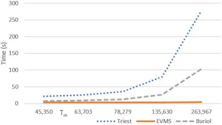
EVMS performs better than the Triest-Base and EVSS in terms of time as well. The reason is that in general, reservoir sampling takes more time than fixed probability sampling (especially when the reservoir size is high). As an example let us consider the the Orkut graph with more than 170 million edges. The EVMS algorithm gives an estimate with pE = 4% in over a minute with Tm = 145000, where as Triest-Base takes over 5 minutes and over 800,000 units of memory
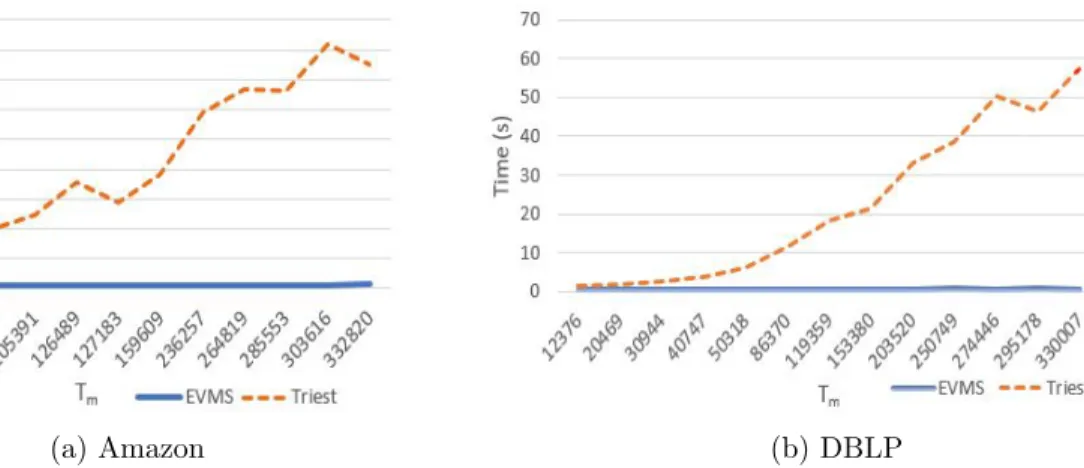
for the achieving the same accuracy. Figure 4.2shows the time taken by both the algorithms for the amazon graph and DBLP graphs. Figure 4.1 shows the time taken by the EVSS,EVMS and Triest-Base algorithms for the As-Skitter graph. The EVMS algorithm takes less than 4s in all cases, whereas the time increases linearly withTm for the Triest-Base and EVSS algorithms.
(a) Amazon (b) DBLP Figure 4.2: Tm vsT ime for Triest-base and EVMS algorithms
4.2.3 EVMS vs Neighborhood Sampling
The base version of neighborhood sampling was implemented. We observed that EVMS al-gorithm has better accuracy compared to the neighborhood sampling alal-gorithm. Moreover, the run-time of the base implementation of the neighborhood sampling algorithm is high. In their work they optimized the run time by doing a batch processing. However batch processing has the disadvantage that we have to wait till the entire stream is processed to obtain a triangle count. More specifically, triangle count can not be monitored continuously. Due to very high running times further analysis and comparison with this algorithm are not reported.
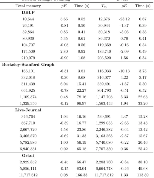
4.2.4 EVMS vs Colorful triangle Counting
The colorful triangle counting algorithm first chooses 1/p many colors and randomly assigns a color to each vertex. Since the vertices are numbered from 0 to n−1, 1/p colors were randomly assigned to integers from 0 ton−1. Then edges whose end points have the same color are placed in the sample. The colorful triangle counting was run by setting thepwith values 0.01, 0.03, 0.05, 0.08, 0.10, 0.17, 0.20. The total memory,Tcused was measured as the total number of edges sampled in
each color. The comparison is done by approximately matching the total memoryTm used by the
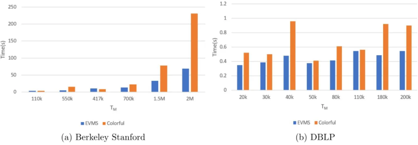
though the time taken is more than EVMS algorithm, the colorful triangle counting gives better accuracy when compared to EVMS. Figure4.3shows the time taken by both the algorithms for the Berkeley Stanford and Amazon graphs.
(a) Berkeley Stanford (b) DBLP
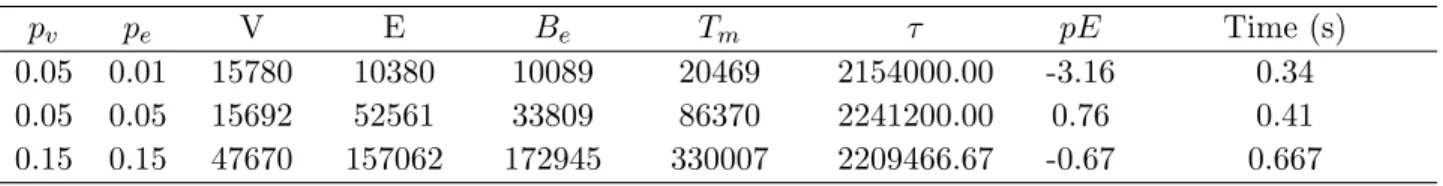
Table 4.3: Results of the EVMS algorithm for various graphs DBLP social network pv pe V E Be Tm τ pE Time (s) 0.05 0.01 15780 10380 10089 20469 2154000.00 -3.16 0.34 0.05 0.05 15692 52561 33809 86370 2241200.00 0.76 0.41 0.15 0.15 47670 157062 172945 330007 2209466.67 -0.67 0.667
Amazon Product Graph
pv pe V E Be Tm τ pE Time (s)
0.15 0.01 50189 9424 15761 25185 691333.33 3.63 0.28
0.05 0.05 16675 46089 20210 66299 648800.00 -2.75 0.33
0.05 0.1 17025 92809 34374 127183 668000.00 0.13 0.40
Berkeley-Stanford web graph
pv pe V E Be Tm τ pE Time (s) 0.05 0.01 34220 66984 249093 316077 67424000.00 4.22 3.17 0.15 0.01 103180 66359 735434 96542 64361333.33 -0.51 6.52 0.05 0.05 34094 332610 402696 735306 64628800.00 -0.10 13.74 As-skitter pv pe V E Be Tm τ pE Time (s) 0.1 0.01 169712 110627 753437 27417 27417000.00 -4.70 4.48 0.01 0.05 16982 555164 121783 676947 28384000.00 -1.34 4.19 0.05 0.1 84387 1108978 748970 1857948 28740000.00 -0.10 14.75 Live-journal pv pe V E Be Tm τ pE Time (s) 0.01 0.01 39834 347209 192482 18577 185770000.00 4.47 15.28 0.15 0.01 599880 347082 2816486 3163568 172709333.33 -2.87 15.67 0.1 0.05 400063 1735031 4005049 887176 177435200.00 -0.22 20.46 Orkut-social network pv pe V E Be Tm τ pE Time (s) 0.01 0.01 30856 1171375 1112385 2283760 622330000.00 -0.84 38.10 0.15 0.01 460448 1171998 16168020 17340018 629705333.33 0.34 66.34 0.1 0.05 306699 5857609 18158724 24016333 627276600.00 -0.05 106.96
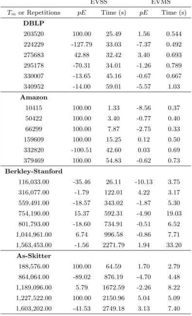
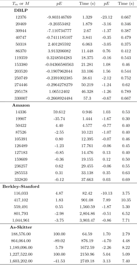
Table 4.4: EVMS vs EVSS sampling
EVSS EVMS
Tm or Repetitions pE Time (s) pE Time (s) DBLP 203520 100.00 25.49 1.56 0.544 224229 -127.79 33.03 -7.37 0.492 275683 42.88 32.42 3.40 0.693 295178 -70.31 34.01 -1.26 0.789 330007 -13.65 45.16 -0.67 0.667 340952 -14.00 59.01 -5.57 1.03 Amazon 10415 100.00 1.33 -8.56 0.37 50422 100.00 3.40 -0.77 0.40 66299 100.00 7.87 -2.75 0.33 159609 100.00 15.25 0.12 0.50 332820 -100.51 42.60 0.03 0.69 379469 100.00 54.83 -0.62 0.73 Berkley-Stanford 116,033.00 -35.46 26.11 -10.13 3.75 316,077.00 -1.79 122.01 4.22 3.17 559,491.00 -18.57 343.02 -1.87 5.30 754,190.00 15.37 592.31 -4.90 19.03 801,793.00 -18.60 734.91 -0.51 6.52 1,044,961.00 6.74 996.58 -0.86 7.71 1,563,453.00 -1.56 2271.79 1.94 33.20 As-Skitter 188,576.00 100.00 64.59 1.70 2.79 864,064.00 -89.02 876.19 -4.70 4.48 1,189,096.00 5.79 1672.59 -2.26 8.22 1,227,522.00 100.00 2150.96 5.04 5.09 1,603,202.00 -41.53 2749.18 3.13 7.40
Table 4.5: EVMS vs Triest Base Triest EVMS TmorM pE Time (s) pE Time (s) DBLP 12376 -9.803146769 1.329 -23.12 0.667 20469 -9.20353482 1.879 -3.16 0.346 30944 -7.110734777 2.67 -1.37 0.387 40747 -0.7411185107 3.841 -0.35 0.479 50318 2.401285592 6.063 -3.05 0.375 86370 3.913206082 11.448 0.76 0.412 119359 0.3248504283 18.375 -0.16 0.543 153380 -0.04366580563 21.281 1.08 0.46 203520 -0.1907962044 33.106 1.56 0.544 250749 -0.2391002385 38.61 -2.12 0.752 274446 -0.2964278279 50.219 -1.24 0.62 295178 1.06512402 46.328 -1.26 0.789 330007 -0.2668924484 57.3 -0.67 0.667 Amazon 14336 59.612 0.946 1.03 0.53 19907 -35.74 1.444 -1.67 0.30 50422 4.40 4.577 -0.77 0.40 87526 -2.55 10.121 -1.07 0.40 105391 0.80 12.395 -0.07 0.46 126489 -1.23 17.761 -0.06 0.45 127183 -0.85 14.476 0.13 0.40 159609 -0.36 19.155 0.12 0.50 236257 0.62 29.455 -0.06 0.55 285553 0.31 33.138 0.35 0.63 332820 -0.12 37.663 0.03 0.69 Berkley-Stanford 116,033 4.87 82.42 -10.13 3.75 417,102 1.83 901.08 7.89 10.35 559,491 0.55 1,560.59 -1.87 5.30 801,793 -2.98 2,804.86 -0.51 6.52 1,044,961 -3.75 3,903.47 -0.86 7.71 As-Skitter 188,576.00 100.00 64.59 1.70 2.79 864,064.00 -89.02 876.19 -4.70 4.48 1,189,096.00 5.79 1672.59 -2.26 8.22 1,227,522.00 100.00 2150.96 5.04 5.09 1,603,202.00 -41.53 2749.18 3.13 7.40
Table 4.6: EVMS vs Colorful triangle counting
Colorful Triangle Counting EVMS
Total memory pE Time (s) Tm pE Time (s) DBLP 10,544 5.65 0.52 12,376 -23.12 0.67 26,191 -0.81 0.50 30,944 -1.37 0.39 52,864 0.85 0.41 50,318 -3.05 0.38 80,930 5.35 0.61 86,370 0.76 0.41 104,707 -0.08 0.56 119,359 -0.16 0.54 174,509 2.80 0.92 183,740 -2.09 0.49 210,079 -0.90 1.08 203,520 1.56 0.54 Berkeley-Stanford Graph 166,101 -6.31 3.81 116,033 -10.13 3.75 332,018 -0.30 8.68 316,077 4.22 3.17 511,439 6.04 15.41 559,491 -1.87 5.30 664,925 -0.78 22.27 801,793 -0.51 6.52 1,109,374 0.48 78.16 1,147,703 5.33 22.63 1,329,356 -0.12 96.97 1,563,453 1.94 33.20 Live-Journal 346,764 1.04 16.16 539,691 4.47 15.28 867,710 -0.39 16.77 1,299,055 -2.65 13.43 2,667,720 4.58 23.86 2,246,382 -0.64 13.42 3,468,870 -0.62 31.33 3,163,568 -2.87 15.67 5,782,986 1.00 56.19 5,740,080 -0.22 20.46 6,940,331 0.02 65.18 7,707,350 0.36 25.42 Orkut 2,929,852 -0.45 56.47 2,283,760 -0.84 38.10 5,856,111 -0.15 83.04 6,664,778 -0.46 49.68 11,717,612 0.08 166.33 11,717,812 1.33 113.89
CHAPTER 5. CONCLUSION AND FUTURE WORK
The thesis presents the Edge vertex Multi Sampling algorithm that has better theoretical bounds
O(m √ ∆V √ T 1 log( ∆V
δ )) than several state of art algorithms. We also verify if the gain seen in the
the-oretical analysis reflects in the experimental analysis. Based on the experiments we can make the following conclusions. The EVMS algorithm has better accuracy and run-times compared to EVSS , Triest-Base and neighborhood sampling, lower accuracy compared to colorful triangle counting. However, EVMS is faster the the colorful triangle counting. The algorithm can be further extended for dynamic streams, where the stream contains deletion edges. Also, the algorithm can be made even faster using the map-reduce technique suggested in R. Pagh et al[18]. Further, the multi-sampling strategy can also be applied to other single multi-sampling techniques like the neighborhood sampling.
[1] Alon, N., Matias, Y., and Szegedy, M. (1996). The space complexity of approximating the frequency moments. ACM Symposium on Theory of Computing, pages 20–29.
[2] Bar-Yossef, Z., Kumar, R., and Sivakumar, D. (2002). Reductions in streaming algorithms, with an application to counting triangles in graphs. In SODA, pages 623–632.
[3] Becchetti, L., Boldi, P., Castillo, C., and Gionis, A. (2008). Efficient semi-streaming algorithms for local triangle counting in massive graphs. In KDD, pages 16–24.
[4] Bott, E. (1957). Family and Social Network: Roles, Norms and External Relationships in Ordinary Urban Families.
[5] Braverman, V., Ostrovsky, R., and Vilenchik, D. (2013). How hard is counting triangles in the streaming model? InICALP, pages 244–254.
[6] Buriol, L. S., Frahling, G., Leonardi, S., Marchetti-Spaccamela, A., and Sohler, C. (2006). Counting triangles in data streams. In SIGMOD, pages 253–262.
[7] Eckmann, J.-P. and Moses, E. (2002). Curvature of co-links uncovers hidden thematic layers in the world wide web. PNAS, 99(9):5825–5829.
[8] Foster, D. V., Foster, J. G., Grassberger, P., and Paczuski, M. (2011). Clustering drives assor-tativity and community structure in ensembles of networks. Phys. Rev. E, 84:066117.
[9] Huang, Z. (2010). Link prediction based on graph topology: The predictive value of generalized clustering coefficient. Social Science Research Network.
[10] Jha, M., Seshadhri, C., and Pinar, A. (2015a). Path sampling: A fast and provable method for estimating 4-vertex subgraph counts. In WWW, pages 495–505.
[11] Jha, M., Seshadhri, C., and Pinar, A. (2015b). A space-efficient streaming algorithm for estimating transitivity and triangle counts using the birthday paradox. TKDD, 9(3):15:1–15:21. [12] Jowhari, H. and Ghodsi, M. (2005). New streaming algorithms for counting triangles in graphs.
In COCOON, pages 710–716.
[13] Kane, D. M., Mehlhorn, K., Sauerwald, T., and Sun, H. (2012). Counting arbitrary subgraphs in data streams. In ICALP, pages 598–609.
[14] Latapy, M. (2008). Main-memory triangle computations for very large (sparse (power-law)) graphs. Theor. Comput. Sci., 407(1-3):458–473.
[15] Leskovec, J. and Krevl, A. (2014). SNAP Datasets: Stanford large network dataset collection. http://snap.stanford.edu/data.
[16] Lim, Y. and Kang, U. (2015). MASCOT: memory-efficient and accurate sampling for count-ing local triangles in graph streams. In Proceedings of the 21th ACM SIGKDD International Conference on Knowledge Discovery and Data Mining, Sydney, NSW, Australia, August 10-13, 2015, pages 685–694.
[17] Manjunath, M., Mehlhorn, K., Panagiotou, K., and H. (2011). Approximate counting of cycles in streams. InESA, pages 677–688.
[18] Pagh, R. and Tsourakakis, C. E. (2012). Colorful triangle counting and a MapReduce imple-mentation. Inf. Process. Lett., 112(7):277–281.
[19] Pavan, A., Tangwongsan, K., Tirthapura, S., and Wu, K.-L. (2013). Counting and sampling triangles from a graph stream. PVLDB, 6(14):1870–1881.
[20] Sala, A., Cao, L., Wilson, C., Zablit, R., Zheng, H., and Zhao, B. Y. (2010). Measurement-calibrated graph models for social network experiments. In WWW, pages 861–870.
[21] Schank, T. and Wagner, D. (2005). Finding, counting and listing all triangles in large graphs, an experimental study. In Experimental and Efficient Algorithms, 4th InternationalWorkshop, WEA 2005, Santorini Island, Greece, May 10-13, 2005, Proceedings, pages 606–609.
[22] Seshadhri, C., Pinar, A., Durak, N., and Kolda, T. G. (2013). The importance of directed triangles with reciprocity: patterns and algorithms. CoRR, abs/1302.6220.
[23] Stefani, L., Epasto, A., Riondato, M., and Upfal, E. (2016). Tri`est: Counting local and global triangles in fully-dynamic streams with fixed memory size. In Proceedings of the 22nd ACM SIGKDD International Conference on Knowledge Discovery and Data Mining, San Francisco, CA, USA, August 13-17, 2016, pages 825–834.
[24] Suri, S. and Vassilvitskii, S. (2011). Counting triangles and the curse of the last reducer. In Proceedings of the 20th International Conference on World Wide Web, WWW 2011, Hyderabad, India, March 28 - April 1, 2011, pages 607–614.
[25] Tsourakakis, C. E. (2008). Fast counting of triangles in large real networks without counting: Algorithms and laws. In ICDM, pages 608–617.
[26] Tsourakakis, C. E., Drineas, P., Michelakis, E., Koutis, I., and Faloutsos, C. (2011a). Spectral counting of triangles via element-wise sparsification and triangle-based link recommendation. Social Netw. Analys. Mining, 1(2):75–81.
[27] Tsourakakis, C. E., Kang, U., Miller, G., and Faloutsos, C. (2009). DOULION: counting triangles in massive graphs with a coin. InProceedings of the 15th ACM SIGKDD International Conference on Knowledge Discovery and Data Mining, Paris, France, June 28 - July 1, 2009, pages 837–846.
[28] Tsourakakis, C. E., Kolountzakis, M., and Miller, G. (2011b). Triangle sparsifiers. J. Graph Algorithms Appl., 15(6):703–726.