A novel HRRP target recognition method based on LSTM and HMM decision-making

A Novel HRRP Target Recognition Method

Based on LSTM and HMM Decision-making

Jun Tu

1

_{, Teng Huang*}

1

_{, Xusong Liu}

1

_{, Fei Gao}

1

_{and Erfu Yang}

2 1_{School of Electronic and Information Engineering, Beihang University}

Beijing, China

2_{Space Mechatronic Systems Technology Laboratory, Department of Design,} Manufacture and Engineering Management, University of Strathclyde

Glasgow G1 1XJ, UK

*Email: [email protected], Abstract—Feature learning is a key step of target

recognition for high-resolution range profile (HRRP). In traditional methods, Hidden Markov Model (HMM) can learn the features of HRRP target aspect information. However, the contextual correlations of HRRPs are ignored due to the independence assumptions in HMM, which brings many limitations to feature learning and weakens the generalization performance. On the contrary, the Long Short-Term Memory (LSTM) network can learn the contextual correlations of HRRPs, but not the target aspect information. To overcome the limitations in these feature learning methods, a new HRRP target recognition method that combines LSTM with HMM decision-making is proposed in this paper. The method consists of two branches: one is target recognition based on HMMs directly; the other is that the latent correlations of HRRPs are extracted by LSTM network and then use HMMs to do target recognition. Finally, the recognition result is obtained by making joint decisions between the two branches. The HRRPs are generated by the inversion of real radar images and the experimental results show that the proposed algorithm outperforms both the HMM and LSTM method.

Keywords-automatic target recognition (ATR); high-resolution range profile (HRRP); deep learning; long short-term memory (LSTM); Hidden Markov Model (HMM)

I. INTRODUCTION

High-resolution range profiles (HRRPs) are one-dimensional (1-D) profiles, which represent the projection of the complex echoes from the target scattering centers onto the radar line of sight (LOS). HRRPs can reflect abundant target structure information, and they are quite useful for target recognition. Compared with the two-dimensional (2-D) synthetic aperture radar (SAR) images [1-3], on the one hand, HRRPs are easier to obtain, store, and process; on the other hand, HRRPs can maintain a certain stability when the target moves, while the SAR image tends to be blurred [4-5]. Therefore, HRRP-based target recognition has always been a hot topic in the field of radar automatic target recognition (ATR) [6-8]. For better recognition performance, it is a crucial issue that how to adequately learn the features from the HRRP data.

In early researches, researchers usually extract statistical features of HRRPs for recognition. As a representative of statistical model [9-10], Hidden Markov Model (HMM) is widely applied to the field of HRRP target recognition [11-14]. For example, HRRP

superresolution scattering center features are modeled by HMM in [11]. The HRRP scattering center features extracted by the RELAX algorithm are modeled by HMM in [12]. What’s more, HMM is not limited to modeling HRRP features which are extracted based on time domain analysis. Zhang et al.[13] used time-frequency domain features of HRRPs to train HMMs. Albrecht et al.[14] used the HRRP energy spectrum features obtained based on frequency domain analysis to train HMMs. HMM is so widely used in this field, because it can clearly describe the statistical features of HRRP which varies with the target aspect angle [9]. What’s more, HMM is capable of modeling time-varying signals like HRRPs. Nevertheless, based on the assumption that there is no memory between echoes, HMM only depends on each state and the corresponding observation object. Hence, contextual correlations of HRRPs are ignored, which weakens the generalization ability of HMM.

To improve model recognition performance, with the development of deep learning technology [15-17], a large of deep network architectures are applied to HRRP target recognition problems [18-19]. As a representative of these architectures, Long Short-Term Memory (LSTM) networks can not only learn the contextual correlations, but also solve the long-term dependency problem with the help of a set of gate structures [20]. Therefore, LSTM showed better performance in recognition and learning features of HRRPs with strong contextual correlations in [21]. In [22], a bidirectional LSTM model is used to learn HRRP features and the algorithm is robust. Nevertheless, the HRRP sequence made up of several HRRPs has certain statistical properties. On the one hand, when the variation of aspect angle between the radar LOS and the target is small, the HRRP sequence has a local stationary characteristic. On the other hand, it is a globally non-stationary sequence when the variation is large [12]. LSTM network is not good at learning the statistical properties.

In order to overcome the limitations in the above feature learning methods for HRRPs, a new target recognition method based on LSTM and HMM decision-making is proposed in this paper. Firstly, the time domain features of HRRPs are extracted to form the feature sequences. The sequences are divided into multiple approximately stationary sequences according to the aspect angles, and then the original HMMs are established. Different classes of models correspond to the different

This research was funded by the National Natural Science Foundation of China, no. 61771027. Dr Yang is supported in part by the Advanced Forming Research Centre (AFRC) and Lightweight Manufacturing Centre(LMC) under the Route to Impact Programme 2019–2020 funded by Innovate UK High Value Manufacturing Catapult [grant no.: AFRC_CATP_1469_R2I-Academy]

Proceedings of the 25th _{International Conference on}

Automation & Computing, Lancaster University, Lancaster UK, 5-7 September 2019

classes of targets. Secondly, an LSTM network is constructed, and the aforementioned extracted time domain features are inputted into the network to learn the contextual correlations of the HRRP sequences. What’s more, improved HMMs are constructed for the output of the LSTM network. Lastly, the final recognition result is obtained by making joint decisions between the original HMMs and the improved HMMs.

The rest of the paper is organized as follows. In Section 2, LSTM network and HMM are reviewed as a preparation. In Section 3, the proposed method is presented in detail. The experiments are performed in Section 4. Finally, the paper is concluded in Section 5.

II. LSTM NETWORK AND HMM

A. LSTM network

The LSTM network is a special Recurrent Neural Network (RNN) which has the same recursiveness as the traditional RNN. Its network architecture is illustrated in Fig. 1 [20].

As shown in Fig. 1, xt is the input of LSTM unit at

time step t. The unit output is consisted of two parts: one is the hidden state ht; the other is the current unit state

which is output to the next unit to form a recursive structure. As can be seen from the recursive relationship between the LSTM units at different time steps, the LSTM network is able to learn the correlations between adjacent samples in the input sequence. Compared to the ordinary RNN, the hidden layer of the LSTM network is no longer the common neural unit, but the LSTM unit with unique memory mode. Each LSTM unit contains a memory cell whose internal structure is demonstrated in Fig. 2 [20].

In Fig. 2, the state of LSTM unit at time step t is recorded as ct. The meanings of xt and ht are the

same as the meanings in Fig. 1 and when the subscript is

t-1 they indicates the previous corresponding values.

Each line represents a complete vector. The combination between different lines represents the connection. The fork means that the original vector is copied and put into different nodes. The structure consisting of the point multiplication operation and the activation function layer in Fig. 2 is called “gate”. It can be clearly seen that there are some well-designed gates in the LSTM cell: input gate

t

i , forget gate ft, output gate ot. The gate structures are

able to remove or add information to the state of the cell and make decisions about the storage, writing and deletion of information in the cell, allowing information through optionally. These operations are performed according to the following formulas:

1 ( [ , ] ), t f t t f f =

σ

W h x⋅ − +b (1) 1 ( [ , ] ), t i t t i i =

σ

W h x⋅ − +b (2) 1 tanh( [ , ]1 ), t t t t c t t c c = ⋅f c− + ⋅i W h x⋅ − +b (3) 1 ( [ , ] ), t o t t o o =

σ

W h x⋅ − +b (4) tanh( ). t t t h o= ⋅ c ₍₅₎ LSTM

Unit LSTMUnit LSTMUnit

h2 ht

x1 h1

x2 xt

...

Figure 1. The structure of LSTM network.

σ tanh tanh σ σ 𝒉𝒉𝒕𝒕 𝒉𝒉𝒕𝒕 𝒄𝒄𝒕𝒕 𝒉𝒉𝒕𝒕−𝟏𝟏 𝒙𝒙𝒕𝒕 𝒄𝒄𝒕𝒕−𝟏𝟏 𝒇𝒇𝒕𝒕 𝒊𝒊𝒕𝒕 𝒐𝒐𝒕𝒕 𝒄𝒄�𝒕𝒕 Figure 2. An LSTM cell.

In these formulas, W_f , W_i, W_c, W_o are the weight matrices connecting to the input signal xt; bf, bi, bc,

o

b are the offset vectors;

σ

is the activation function which is generally the sigmoid function [20]. As can be seen from these relationships, the gate structure enables truly useful information to function for the weights adjustment over the long term, while unnecessary information is forgotten in the short term.

When HRRPs are inputted as x_t , HRRPs are

sequenced with aspect angles in order and fed into LSTM with varying time steps for feature learning. Then, the potential correlations within the HRRP sequences can be easily extracted using the LSTM network. Nevertheless, if we only use LSTM there will be some limitations in the feature learning application of HRRP sequences, since the HRRP sequences have strong statistical features and the learning of statistical features is not the speciality of LSTM. In comparison, HMM has more advantages in this regard.

B. Hidden Markov Model

HMM is a probabilistic statistical model, which contains two stochastic processes: one is a Markov chain characterized by states and transition probabilities; the other describes the relationships between observations and states. HMM contains observable states and hidden states. The transitions between hidden states can only be perceived by the observable states, but not being observed directly [9].

A HMM can be represented as

λ

={ , , }A B

π

. A is the state transition matrix which describes the transition probabilities between states. B is the observation probability matrix which describes the conditional probabilities of one observable state given the current hidden state. When the HMM is a continuous HMM, B is a group of continuous probability density functions.

π

is the initial probability distribution for the states. For HRRP sequences, the change of HRRP sequences can be approximated as a stationary stochastic process when the

aspect angle changes within a small range, so a state in the HMM can represent several adjacent HRRPs. If the aspect angle changes within a large range, the HRRP sequences can be regarded as non-stationary random processes, which can be represented by the Markov chains describing the state transition in the HMMs [12]. The construction process of HMMs is demonstrated in Fig. 3.

When HMMs are constructed for HRRPs, the states of HRRPs are evenly divided according to the aspect angles. Each state covers a certain range of target aspect angles of several HRRPs. Due to the continuity of the radar orientation when HRRPs are acquired, the state transition can only occur between adjacent states or themselves. The observation sequences are the HRRP sequences consisting of HRRPs in different aspect angles. The observation probability density function can be initially estimated by a Gaussian function. What’s more, by assuming that the HRRP distribution is uniform across different aspect angles, it is easy to acquire the initial estimate of other parameters such as state transition probabilities [23]. And then, Baum-Welch algorithm is applied to the observation sequences in the training set. According to the algorithm, the most suitable parameter values above can be found by iterative fine tuning based on the maximum likelihood estimation. At last, a trained model is obtained and can be used for recognition [9].

The applicability of HMM to the feature learning of HRRP sequences is not only from the statistical features of them, but also from the statistical modeling ability of HMM itself to the time series structure like the time domain features extracted from HRRPs. In traditional studies, HMM did show its advantages of modeling for the recognition of HRRPs [11-14]. However, there are several strict assumptions in HMM: the output is only related to the current state, and the current state is only related to the previous state. In fact, due to the continuous motion of the airborne radar, there are large correlations between the HRRPs of the adjacent echoes, and the HRRPs with different aspect angles are not mutually independent. What’s more, when the states of HRRPs are divided according to the aspect angles, the relationship between these states is different from the assumption of the HMM. Therefore, the strict assumptions in HMM lead to some limitations in the application of HRRP recognition. In order to overcome these limitations, this paper uses the LSTM network to pre-extract the contextual correlations of the HRRP sequences. The details of the proposed method are in the next section.

s1 a12 s2 a23 sL a11 a22 al-1l all

……

……

HRRPs

aspect angle range

HMM states

θ1 θ2 θl

transition probabilities

a21 a32 all-1

Figure 3. The construction process of HMMs.

III. MODELING AND TARGET RECOGNITION

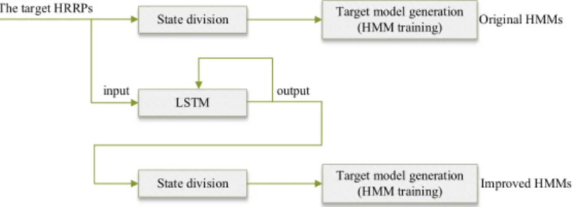
The proposed method consists of two steps: modeling and recognizing. There are two branches in the process of modeling. In the first branch, the HRRP sequences are divided according to their respective aspect angles and then the original HMMs are established, as shown in Fig. 4. In the second branch, the HRRP sequences are fed into an LSTM network for training purpose, and the improved HMMs are constructed to model the output sequences. At each branch, each class of target has one corresponding model. There are also two branches in the process of recognizing, as shown in Fig. 5. On one side, the test sequences are fed into the trained LSTM network. Then the outputs of LSTM network are fed into the improved HMMs to calculate the conditional probabilities of the outputs given each model. On the other side, the test sequences are directly fed into the original HMMs to calculate the probabilities. Finally, the original HMMs and the improved HMMs make joint decisions, and the class of the model corresponding to the maximum probability is the recognition result.

A. State division and HMMs construction

The division of the HMM states is determined according to the corresponding aspect angles of the SAR images which fully cover 360 degrees. The specific number of the partitions of HMM states must be neither too small nor too large, so that all variations of the target features can be sufficiently modeled and enough features can be trained. According to [12], the recognition performance is the best when the number of states is 120. Thus, the data are divided into 120 states and the angular resolution is 3 degrees.

State division Target model generation_{(HMM training)}

LSTM

input output

State division Target model generation_{(HMM training)}

Original HMMs

Improved HMMs The target HRRPs

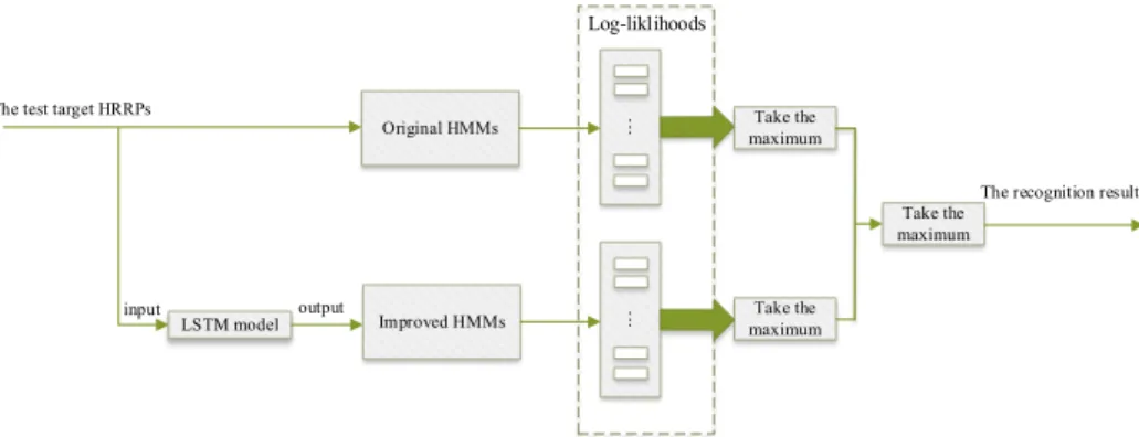
The test target HRRPs

The recognition result Original HMMs Improved HMMs LSTM model input output Log-liklihoods Take the maximum ... ... Take the maximum Take the maximum

Figure 5. The flow chart of recognition.

There are usually two choices of discrete HMMs and continuous HMMs. On the one hand, the output of the former are discrete random variables so the model is simple. On the other hand, there are large quantization errors in discrete HMMs so that the distortion inherent in the quantization of HRRPs feature vectors cannot be avoided [9]. Therefore, continuous Gaussian HMMs are adopted here. More precisely, probability density function which describes the relationship between the observed values and the hidden states is fitted by a superposition of a plurality of Gaussian functions.

According to the description in Section 2.2 and the detailed description in [23], the parameters of trained HMMs specifically reflects the statistic features of various targets. So the HMMs can be directly used for target recognition. The HRRPs of one target are input into each HMM to calculate the likelihood values, and then the class of the HMMs corresponding to the maximum likelihood value is the recognition result of the target.

B. Model fusion and joint decision-making

The modeling process consists of two branches. On one side, the HRRP sequences are used to establish original HMMs. on the other side, the HRRP sequences are fed into the LSTM network for training purpose. The recursiveness of the LSTM network is reflected in Fig. 4, and the primary purpose of LSTM is to make full use of the contextual correlations between the HRRP sequences. When the training process is finished, the output of the LSTM network are utilized as new sequences whose states are divided according to the aspect angles, and then the improved HMMs are generated. It is worth noting that the original HMMs are necessary despite the existence of improved HMMs. The reason is that the noise influence in the training data are amplified by too many learning features when LSTM network is connected to the HMMs, so that the models get overfitting easily and the generalization ability of the models is weakened. However, these effects can be effectively alleviated if the improved HMMs are used together with the original HMMs, as illustrated in Fig. 5.

In the target recognition process, the HRRP sequences generated by the test target images are first fed into each model to calculate the likelihood probability value. Obviously, when the improved HMMs are used for recognition, the sequences should be first input to the previously trained LSTM model whose output sequences are fed into the improved HMMs. On the contrary, the

original HMMs directly receive the HRRP sequences. Then for each class of model, a corresponding likelihood probability value of the target is observed. After that, a class of model is determined as candidate model in original HMMs based on the maximum likelihood probabilities, and a candidate model in improved HMMs is determined too. Finally, the conditional probabilities of the test sequence given the two candidate HMMs are compared, and the class of model corresponding to the maximum value is the recognition result.

In fact, a method based on decision-making is employed in the final step. HMMs are constructed using maximum likelihood estimation, so the size of the likelihood probabilities here reflect the ability of the HMM group to classify the input test sequences. For each target data set, the signal-to-noise ratio is different. It is obvious that the improved HMMs with more learning features have stronger recognition ability when the input data have a high signal-to-noise ratio. On the contrary, the original HMMs are better when the signal-to-noise ratio is low. When recognizing specific targets, it is automatically eliminated that the group of models with weak recognition ability due to the low likelihood probability under each class of model. At the same time, the input sequences perform prominent likelihood probability under a certain HMM in another group of HMMs, and then the target is recognized as this class. This is equivalent to a mechanism of survival of the fittest. Such a method based on decision-making enables all the models built to be made full use of, and it is simple and easy to implement.

IV. EXPERIMENTS

A. Database and data preprocessing

The experiments are performed on the Moving and Stationary Target Acquisition and Recognition (MSTAR) database, which is a standard database for evaluating the performance of ATR algorithms [24]. The MSTAR database contains ten types of targets and the corresponding optical images are shown in Fig. 6.

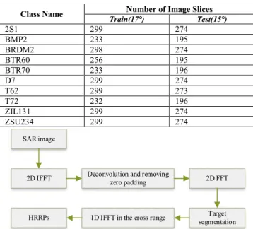
TABLE I. THE NAMES OF THE TARGETS OF EACH CLASS IN THE TRAINING SAMPLES AND THE TEST SAMPLES AND THE NUMBER OF

IMAGE SLICES

Class Name _Train(17°) Number of Image Slices _Test(15°)

2S1 299 274 BMP2 233 195 BRDM2 298 274 BTR60 256 195 BTR70 233 196 D7 299 274 T62 299 273 T72 232 196 ZIL131 299 274 ZSU234 299 274 SAR image

2D IFFT Deconvolution and removing _{zero padding} 2D FFT

Target segmentation 1D IFFT in the cross range

HRRPs

Figure 7. The procedure from a SAR image to HRRPs.

Each class of targets contains images collected at 15° and 17° depression angles. In this paper, the training set consists of the 17° data, and the testing set consists of the 15° data. For the images of each target, the range of their aspect angles basically covers 360 degrees. Table 1 shows the name of each target and the number of image slices in the training and test sets.

The transformation operations for converting SAR images into HRRPs are briefly shown in Fig. 7. And the detailed procedure is given in [12]. For the simplicity of process and removing useless noise as much as possible, the HRRPs are uniformly cropped to 64 pixels long. After cropping, the modulo operation is performed to extract time domain features.

To prepare for the experiments, there are several simple steps for the transition from the processed HRRPs to the final HRRP sequences. Firstly, each five HRRPs are chosen from each SAR image slice. Specifically, a hundred HRRPs can be generated from one SAR image, and each final HRRP is the average of twenty adjacent HRRPs. Then, a HRRP sequence is the sequence of these processed HRRPs with aspect angles in order. And only one HRRP sequence for each target class exists in our HMMs. Finally, for our LSTM network, all classes of HRRP sequences are synthesized into one HRRP sequence with classes in order.

B. Experimental results and analysis

In order to make a more detailed analysis of the effects of the LSTM network and HMM, four methods are compared each other. The first experiment is to construct HMMs directly for HRRP sequences [14]. In the second experiment, the HRRP sequences are trained and recognized directly by a single LSTM network, and the softmax classifier is adopted. The third experiment is to directly connect an LSTM network to the HMMs. The

method in the third experiment is equivalent to the rest of the proposed method whose final joint decision-making part is removed. The fourth experiment uses the proposed method in this paper.

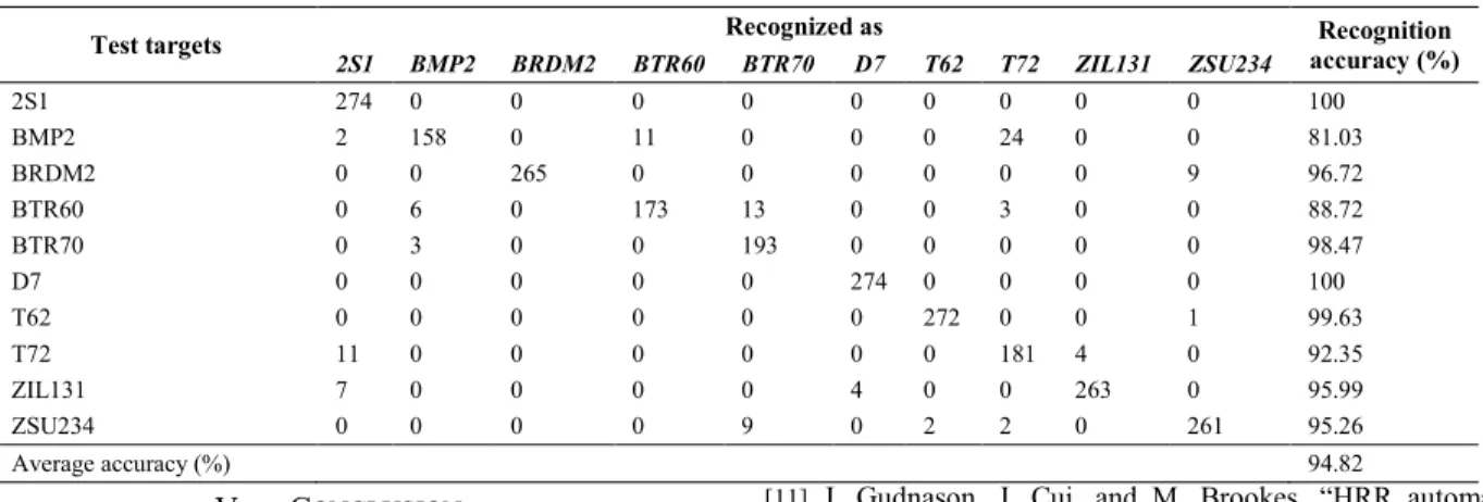
For detailed comparison, different percentages of samples are selected from the training set, and the recognition accuracy of the four methods is shown in Fig. 8. For each method, the recognition accuracy rises with the increasing percentage of the training samples. What’s more, the recognition accuracy of the proposed method is higher than the others. When all samples are involved in the training, the specific results of recognition accuracy are as follows. It is 84.49% for the traditional HMMs and 90.18% for the single LSTM network. It is 90.26% when an LSTM network is directly connected to the HMMs, while it is 94.82% for the proposed method. The specific experimental results of the proposed method are shown in Table 2. In traditional HMMs, the Markov assumption makes the performance is weaker than in LSTM network. And the performance in the proposed method is the best, because the elaborate combination of HMMs and LSTM network makes the contextual correlations of HRRPs and the target aspect information can be effectively learned simultaneously.

From Fig. 8, it can also be seen that the single LSTM network and the HMM methods are sensitive to the number of training samples. Relatively speaking, the proposed method shows a certain robustness when the number of training samples is reduced. Moreover, it can be found that when LSTM network is directly connected to the HMMs in the third experiment, the model performance is superior to the single LSTM network and the HMM methods only when the number of training samples is insufficient. However, when the number of training samples is sufficient, the generalization ability of the model in the third experiment is basically consistent with the ability of the single LSTM network. It can be considered that when the LSTM network is directly connected to the HMMs, more noises are learned than when using the single LSTM network and the HMM methods. It turns out that the generalization ability of the model is weak. On the contrary, this effect is effectively suppressed in the fourth experiment in which the decision-making is adopted for two groups of HMMs. All of these indicate that the performance of the proposed method is impressive.

Figure 8. The recognition accuracy of different methods. percentage of training samples(%)

0 10 20 30 40 50 60 70 80 90 100 recognition accuracy(%) 55 60 65 70 75 80 85 90 95 100 HMM LSTM LSTM+HMM(connect directly) LSTM+HMM(proposed method)

TABLE II. THE RECOGNITION RESULT OF THE PROPOSED METHOD

Test targets _{2S1 BMP2 BRDM2 BTR60 BTR70} Recognized as _{D7 T62 T72 ZIL131 ZSU234 accuracy (%)} Recognition

2S1 274 0 0 0 0 0 0 0 0 0 100 BMP2 2 158 0 11 0 0 0 24 0 0 81.03 BRDM2 0 0 265 0 0 0 0 0 0 9 96.72 BTR60 0 6 0 173 13 0 0 3 0 0 88.72 BTR70 0 3 0 0 193 0 0 0 0 0 98.47 D7 0 0 0 0 0 274 0 0 0 0 100 T62 0 0 0 0 0 0 272 0 0 1 99.63 T72 11 0 0 0 0 0 0 181 4 0 92.35 ZIL131 7 0 0 0 0 4 0 0 263 0 95.99 ZSU234 0 0 0 0 9 0 2 2 0 261 95.26 Average accuracy (%) 94.82 V. CONCLUSION

Aiming at the target recognition of HRRPs, a new target recognition method which integrates LSTM and HMM is proposed in this paper. This method can not only learn the contextual correlations of HRRPs, but also utilize the target aspect information. The HRRPs of 10-class targets are generated by the inversion of real SAR images. The experimental results show that the proposed method can effectively improve the generalization ability of the model and the average recognition accuracy reaches over 94%.

REFERENCES

[1] F. Gao et al, “A novel semi-supervised learning method based on fast search and density peaks,” Complexity, 2019.

[2] F. M a, F. Gao, J. Sun, H. Zhou, and A. Hussain, “Weakly supervised segmentation of SAR imagery using superpixel and hierarchically adversarial CRF,” Remote Sensing, 2019. 11(5): pp. 512

[3] F. Gao et al, “Visual saliency modeling for river detection in high-resolution SAR imagery,” IEEE Access, 2018. 6: pp. 1000-1014.

[4] S. P. Jacobs, J. A. O’Sullivan, “Automatic target recognition using sequences of high resolution radar range-profiles,” IEEE Transactions on Aerospace and Electronic Systems, 2000. 36(2): pp. 364-381.

[5] S. K. Wong, “High range resolution profiles as motion-invariant features for moving ground targets identification in SAR-based automatic target recognition,” IEEE Transactions on Aerospace and Electronic Systems, 2009. 45(3): pp. 1017-1039.

[6] Y. Jiang, Y. Li, J. Cai, Y. Wang, and J. Xu, “Robust automatic target recognition via HRRP sequence based on scatterer matching,” in Sensors, 2018. 18(2): pp. 593.

[7] X. Peng, X. Gao, and X. Li, “An infinite classification RBM model for radar HRRP recognition,” in 2017 International Joint Conference on Neural Networks (IJCNN). 2017.

[8] X. Peng, X. Gao, Y. Zhang, and X. Li, “An adaptive feature learning model for sequential radar high resolution range profile recognition,” in Sensors, 2017. 17(7): pp. 1675.

[9] L. R. Rabiner, “A tutorial on hidden Markov models and selected applications in speech recognition,” Proceedings of the IEEE, 1989. 77(2): pp. 257-286.

[10] S. E. Levinson, “Continuously variable duration hidden Markov models for automatic speech recognition,” Comput. Speech Lang., 1986. 1(1): pp. 29-45.

[11] J. Gudnason, J. Cui, and M. Brookes, “HRR automatic target recognition from superresolution scattering center features,” IEEE Transactions on Aerospace and Electronic Systems, 2009. 45(4): pp. 1512-1524.

[12] X. Liao, P. Runkle, and L. Carin, “Identification of ground targets from sequential high-range-resolution radar signatures,” IEEE Transactions on Aerospace and Electronic Systems, 2002. 38(4): pp. 1230-1242.

[13] X. Zhang, Z. Liu, S. Liu, and G. Li, “Time-Frequency feature extraction of HRRP using AGR and NMF for SAR ATR,” Journal of Electrical and Computer Engineering, 2015. 36: pp. 1-10.

[14] T. W. Albrecht, and S. C. Gustafson, “Hidden Markov models for classifying SAR target images,” Def. Secur. Int. Soc. Opt. Photonics, 2004, pp. 302-308.

[15] F. Gao et al, “A novel active semisupervised convolutional neural network algorithm for SAR image recognition,” Computational Intelligence and Neuroscience, 2017, 1-8.

[16] C. Luo, L. Yu and P. Ren. “A Vision-Aided Approach to Perching a Bioinspired Unmanned Aerial Vehicle.” IEEE Transactions on Industrial Electronics, 2018. 65: pp. 3976-3984.

[17] F. Gao et al, “A new algorithm of SAR image target recognition based on improved deep convolutional neural network,” Cognitive Computation, 2018.

[18] L. Yuan, "A time-frequency feature fusion algorithm based on neural network for HRRP," Progress In Electromagnetics Research M, 2017. 55: pp. 63-71.

[19] M. Shen, and B. Chen, “Radar HRRP target recognition with recurrent convolutional neural networks,” in Intelligence Science and Big Data Engineering. 2018.

[20] S. Hochreiter, and J. Schmidhuber, “Long short-term memory,” Neural computation, 1997. 9(8): pp. 1735-1780.

[21] V. Jithesh, M. J. Sagayaraj, and K. G. Srinivasa, “LSTM recurrent neural networks for high resolution range profile based radar target classification,” in 2017 3rd International Conference on Computational Intelligence and Communication Technology (CICT). 2017.

[22] B. Xu, B. Chen, J. Liu, P. Wang and H. Liu, “Radar HRRP target recognition by the bidirectional LSTM model,” Xi'an Dianzi Keji Daxue Xuebao/Journal of Xidian University, 2019. 46(2): pp. 29-34.

[23] P. Runkle, P. Bharadwaj, L. Couchman, and L. Carin, “Hidden Markov models for multiaspect target classification,” IEEE Transactions on Signal Processing, 1999. 47(7): pp. 2035-2040.

[24] T. D. Ross, S. W. Worrell, V. J. Velten, J. C. Mossing, and M. L. Bryant, “Standard SAR ATR evaluation experiments using the MSTAR public release data set,” in Aerospace/Defense Sensing and Controls. 1998: SPIE.8.