Abstract
The analysis of nickel metal hydride (Ni-MH) battery
performance is very important for automotive researchers and manufacturers. The performance of a battery can be described as a direct consequence of various chemical and physical phenomena taking place inside the container. In this paper, a physics-based model of a Ni-MH battery will be presented. To analyze its performance, the efficiency of the battery is chosen as the performance measure, which is defined as the ratio of the energy output from the battery and the energy input to the battery while charging.
Parametric sensitivity analysis will be used to generate sensitivity information for the state variables of the model. The generated information will be used to showcase how sensitivity information can be used to identify unique model behavior and how it can be used to optimize the capacity of the battery. The results will be validated using a finite difference formulation.
Introduction
There are several different approaches that are used to model car batteries. Most of them can be separated in two main categories. The first approach, also known as the circuit-based approach, tries to model the behavior of the battery as an electric circuit, (Salameh et al. [6], Chen and Rinćon-Mora [11] and Seaman and McPhee [8]). This results in a conceptually simple model. However in this approach, the actual physical parameters stay hidden and there is no explicit relationship between the model parameters and the battery parameters. This is precisely the point where the benefit of using a chemistry-based approach becomes apparent. In this second approach, the actual chemical reactions and other
electrochemical processes inside the battery are captured (Newman et al. [2], [3], [4], Dao et al. [7], Wu et al. [5], and
Banerjee et al. [9]). Due to its dominance in hybrid vehicles, a Ni-MH battery has been chosen for analysis in this paper. The main objective of this work is to perform analytical sensitivity analysis on a physics-based model of a nickel metal hydride battery. The Ni-MH battery model presented here is based on the battery model presented in Wu et al. [5] and Banerjee et al. [9]. This chemistry-based battery model allows users to access physical parameters of the battery directly, which makes this model suitable for design optimization.
Direct differentiation is used to generate the sensitivity
equations from the governing equations, which are then solved to evaluate the sensitivities of the state variables with respect to the model parameters. In this paper, the feasibility of the use of sensitivity information for the optimization of NiMH battery model has been discussed.
Modelling of NI-MH Batteries
To capture the electro-chemical phenomenon inside the battery, one needs to start from the basic chemical reactions taking place at the individual electrodes. For this model the following chemical reactions are considered.
Main reaction on positive electrode:
(1) Side reaction on positive electrode:
(2)
Physics-Based Models, Sensitivity Analysis, and
Optimization of Automotive Batteries
Published 04/01/20142014-01-1865Joydeep Banerjee and John McPhee
Univ. of WaterlooPaul Goossens and Thanh-Son Dao
MaplesoftCITATION: Banerjee, J., McPhee, J., Goossens, P., and Dao, T., "Physics-Based Models, Sensitivity Analysis, and Optimization of Automotive Batteries," SAE Technical Paper 2014-01-1865, 2014, doi:10.4271/2014-01-1865. Copyright © 2014 SAE International
Main reaction on negative electrode:
(3) Side reaction on negative electrode:
(4)
The metal M in the negative electrode is an inter-metallic compound, usually a rare earth compound.
Governing Equations
To model these reactions the effects of two important quantities, that define the generation of the electromotive forces, must be captured properly. The first quantity is known as the open circuit potential difference and is given by the Nernst equation, Equations (5), (6), (7). The quantity ϕ denotes the thermodynamically predicted potential difference of the corresponding Red-ox reactions.
(5)
(6)
(7)
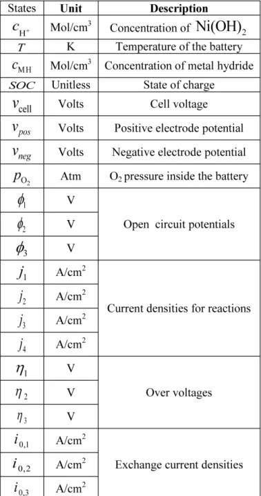
The quantities used in the equations (5), (6), (7) are
summarized in Table 1 and 2. Detailed description of the terms can be found in Banerjee et al. [9].
Apart from the thermodynamically predicted potential difference, the other important quantity in this context is the over potential, which can be directly related to the rate of chemical reactions using the Butler-Volmer equations.
(8)
where i = 1,2,3 are for the reactions given in equations (1), (2), (3). The quantities i0,i are the exchange current densities that are functions of the reactant concentrations and the operating temperature. The exchange current densities are defined at a reference concentration and temperature. But for the purpose of the model, it must be adjusted dynamically to reflect the effects of changing temperature and reactant concentration. The following equations are used for this purpose.
(9)
(10)
(11)
For the oxygen reduction reaction on the negative electrode, i.e. the reaction shown in equation (4), the expression shown in equation (12) is used for the current density. This acts as a limiting current equation. The model parameters used in these equations are summarized in Table 2.
(12)
The battery current can be calculated from the current densities of the reactions at the electrodes.
The mass balance equations for the cell are
(14)
(15)
The closed circuit voltage available from the cell can be calculated as
(16)
Where vpos and vneg are the net potential difference between the electrode and the electrolyte solution for the positive and negative electrodes respectively and can be calculated from the open circuit potential differences, i.e. equations (5), (6), (7), and the over-potentials, i.e. equations (8), (12).
(17)
The energy balance of the whole cell is described by the equation given below.
(18) For the purpose of analysis it is also useful to define an additional state variable which would represent the state of charge (SOC) of the battery. Mathematically it can be expressed as a function of the concentration of Ni(OH)2.
(19)
As mentioned before the current work is based on the model by Wu et al. [5] and Banerjee et al. [9]. The model presented here has the following differences:
• The hysteresis potential behavior is excluded
• Corrected expressions are used for the cell voltage and the over voltages.
• Equations shown in (17) are added to define the relationship of the over voltages.
• In equation (18), only the absolute value of icell × vcell is considered to rule out the possibility of negative values of the resistive thermal losses.
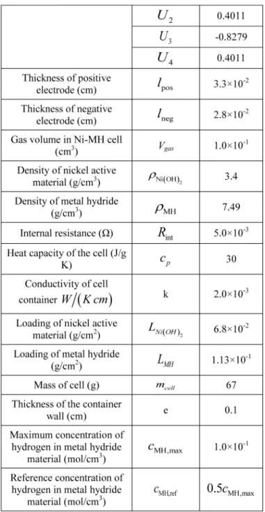
The state variables used in the equations presented above are given in Table 1. The various model parameters used in the equations were measured from a 3.9 Amp-h VARTA Ni-MH battery at the Ford Motor Company Scientific Research Laboratory (Wu et al. [5]), and are summarized in Table 2. Further details can be found in Banerjee et al. [9].
Structure of the Model
At this point it is necessary to identify the nature and structure of the system of governing equations in order to simulate and analyze the model. In this model there are 21 time-dependent entities, i.e. states denoted by {x(t)}. They are described and listed in Table 1. Equations (14) - (15) and (18) are first-order differential equations and the rest are algebraic, together comprising a system of first-order differential algebraic equations (DAEs). The structure of the system can be expressed as
(20) where Φ is the vector of algebraic constraint equations, i.e. functions of {x(t)} and the model parameters {b}. The differential variables {q(t)}are a subset of the generalized states as shown in equation (21).
(21)
To solve the system using numerical methods, consistent initial values of all the generalized states need to be specified.
Table 1. List of generalized states
For a DAE system, the initial conditions must be properly specified so that they satisfy all the constraint equations of the system. However, the four differential variables are
independent and can be assigned arbitrarily. Table 3 shows the initial conditions used for the simulation used in this paper. The rest of the initial values can be obtained by solving the
algebraic constraints.
Table 2. List of Battery parameters
Simulation
The input to the model is the current passing through the battery. Positive values of icell denote the discharging process, where negative values denote the charging phase. Although the quantity icell can be a function of time, for this study we have assumed a constant value for both charging and discharging processes.
The choice of initial conditions reflects the type of physical scenario being simulated. Table 3 lists the values used as initial conditions for the charging process.
Table 3. Initial values used to simulate the charging process
For this study, the initial values of the concentrations are chosen to correspond to an initial state of charge of 0.01. The integration is continued until a state of charge of 0.99 is achieved and the subsequent simulation of discharge is continued until the state of charge comes down to the initial value of 0.01.
At this point, it is necessary to provide a brief description of the simulation environment used in this study.
Maple
Maple is a general-purpose computer algebra system developed and marketed by Waterloo Maple Inc. It
incorporates a dynamically-typed programming language that resembles Pascal. There are provisions for interfacing with C, Fortran, Java and Matlab. The heart of Maple is a kernel written in C. This provides the Maple language. Most mathematical functionalities are provided by libraries. The usual user interface is written in Java.
The main feature of Maple is the ability to manipulate symbolic equations and expressions. It contains a very large library of symbolic operations. Simplification and modification of symbolic expression are routinely done by Maple. Apart from the symbolic capabilities, Maple can also be used for numerical simulations. Advanced numerical routines allow users to solve complicated large systems of ODEs and DAEs using a variety of different algorithms.
Because of its excellent symbolic and numeric capabilities, Maple can be used to simulate dynamic models of electro-chemical systems. In this study, Maple has been used to perform sensitivity analysis and design optimization on the presented model.
MapleSim
MapleSim is a multi-domain modeling and simulation tool developed by Maplesoft Inc. It is capable of simulating electrical, electronic, mechanical, hydraulic and magnetic systems. The input to the software is the description of the system using components from a central library that can be drag-dropped on to a worksheet to build an acausal system model.
MapleSim is built upon Maple, which enables it to perform very effective symbolic simplifications of the generated equations. Also, using Maple's DAE and ODE solvers, it can simulate and plot the output of the models in an interactive
three-dimensional environment. It can also perform post-processing on the generated data using predefined templates.
Apart from the built-in library of standard components, MapleSim allows users to create custom components for user specific implementation. These custom components are based on the Maple language and can be readily included in models created using MapleSim's standard components. It is also possible to create custom components based on Modelica code.
The model presented here has been implemented in MapleSim™ as a custom component. In this way the model can be used as a sub-system for various applications. Organization of Computation
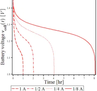
The model implemented in MapleSim is first simulated with different values of constant currents to simulate charging and discharging operations. Figures 1 and 2 shows the resulting plots where the variation of vcell is plotted against time for both charging and discharging scenarios.
Figure 1. Variation of vcell for different values of charging current (Charging operation SOC = 0.01 to 0.99)
For the validation of the model behavior, the charging and discharging characteristics were compared to that obtained by experiments. The experimental data was measured at A & D Technology in Ann Arbor, Michigan, USA. Figure 3 shows the comparison of the experimental and simulated behavior of the system. It illustrates the congruity of the simulated charge discharge behavior and the experimentally obtained data. The plot shown in this figure is obtained by simulating the model using a constant icell = 0.2 A. The plots clearly show that the model is able to capture the dynamic behavior of a NiMH battery with reasonable amount of accuracy.
Figure 2. Variation of vcell for different values of discharging current (SOC 0.99..0.01)
Figure 3. Comparison of model behavior with experimental data for validation purposes
Please note that the model parameters shown in table 2 do not correspond to the battery used for the experimental validation in the earlier paper. The parameters used for the model validation as shown in figure 3 were obtained using parameter identification procedures. The purpose of figure 3 is to demonstrate that the model has indeed been validated previously for actual batteries.
Figure 3 also demonstrates the effect of the internal resistance of the battery. By close observation of figure 3, it can be clearly seen that the final value of vcell achieved after the charging process is slightly higher than the initial value of vcell at the beginning of the discharge phase. This drop in potential difference is caused by the potential drop across the internal resistance that is inherent to the system.
Figure 4. Differences between the charging and discharging curves for different values of current icell.
The losses incurred in the simulated process of charging and discharging of the cell are illustrated in figure 4, where the charging and discharging characteristics are plotted on each other for different values of charging/discharging currents. The differences in the curves clearly identify the amount of energy that is lost in the process.
Sensitivity Analysis
To evaluate the sensitivity of any objective function with respect to the model parameters, one needs to evaluate the
sensitivities of the state variables with respect to the model parameters first. These quantities can be evaluated by solving the sensitivity system which can be readily obtained from the governing equation (20) through direct differentiation. By differentiating equation (20) with respect to an arbitrary scalar model parameter bj and using the chain rule of differentiation equation (22) is obtained.
(22)
In the above expression, the subscripts represent partial differentiation and the symbol refers to the vector being kept constant during the differentiation.
From equations (14), (15) and (18) it is apparent that M is an identity matrix. From this it follows that
(23)
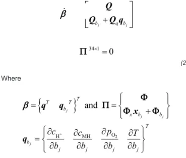
Substituting (23)|into equation (22) a simplified set of DAEs for the sensitivity system is obtained.
(24)
By combining equations (24) and (20) a combined set of DAE is obtained
(25)
Where
(26)
Equation|(25), when solved yields the values of all the state variables and their sensitivities with respect to the model parameter bj.
Figure 5. The variation of the sensitivity of vcell with respect to different model parameters
In this study, the combined set of DAE illustrated in equation (25) is solved numerically in Maple to evaluate the sensitivities of the state variables. The current icell is kept constant at 2A for both charging and discharging phases and the simulation is continued from SOC = 0.01 to SOC = 0.99 and back.
The dsolve[numeric] routine from Maple 16 is used for the simulation. The stiff rosenbrock_dae solver was used with maximum function evaluation set at maxfun=300000 with default error tolerance of ε = 10−6. It was observed that the
value of maxfun is important for the successful completion of the simulation. Figure 5 shows the variation of the sensitivity of vcell with respect to different model parameters for a charging process from SOC = 0.01 to SOC = 0.99.
The plots shown in figure 5 illustrate the relative effects of the model parameters on the battery behavior. It clearly identifies the wall thickness of the cell to have the least effect on the variation of vcell. On the other hand the ambient temperature Ta is shown to have a larger albeit a fluctuating effect on vcell.
Design Optimization
Design optimization requires the minimization or maximization of an objective function that is usually a function of the generalized states and the model parameters. For example, the total available energy of the battery during a discharge process is considered here as the objective function.
(27)
The total available energy from the battery depends on many factors. To ensure standardization, in this analysis it is assumed that the battery is being discharged from the state of charge SOC = 0.99 to a state of charge SOC = 0.01. The objective of the optimization process is to find the set of model parameters that enables the user to harness the maximum amount of energy from the battery given an initial state of full charge.
Gradient-based algorithms can be used to perform the optimization. These methods require the derivatives of the objective function to be optimized. This derivative is evaluated by differentiating the objective function with respect to the model parameter under study. Equation (28) shows the differentiated expression of the objective function shown in equation (27).
(28)
Numerical solution of equation (25) yields the values of vcell and its sensitivity as functions of time. Using numerical integration, equation (28) can be evaluated to yield the sensitivity of the objective function, which can subsequently be used in the optimization procedure.
It should be noted that, for a general situation where the model parameters do affect the integration limits, equation (28) is bound to give erroneous results for the sensitivity data. However, for specific problems and model parameters, these
effects might be numerically negligible. Therefore to ensure accuracy, the results of the optimization must be carefully examined to rule out any inconsistencies introduced by this approximation.
Example Problem
To illustrate the process, a sample optimization problem will be presented in this section: to maximize the amount of energy that can be harnessed from a NiMH battery in a state of full charge.
The model parameters chosen for the optimization are the surface areas of the positive and negative electrodes (Apos and Aneg), and the concentration of the electrolyte, denoted by ce. The purpose of the optimization is to identify optimal values of the model parameters Apos, Aneg, and ce that maximize the objective function given in equation (27), and satisfy the following constraints.
(29) The optimization was performed in Maple, using a first-order gradient descent algorithm. At every step, the gradient of the objective function is evaluated using equation (28) and the corresponding system is simulated by numerically solving equation (25). The results of the optimization process are presented below.
Optimization Results
During the optimization iterations, the values of the selected model parameters were found to settle towards the boundaries of the constraint limits. This fact can be clearly illustrated by plotting the sensitivities of the objective function with respect to the model parameters.
Figure 6. The variation of the sensitivity of Edischarge with respect to the
Figure 6 shows the variation of the sensitivity of the objective function with respect to the model parameter Aneg, which represents the area of the negative electrode.
The plot clearly identifies a decrease in the objective function with an increase in the model parameter's value. Also since the curve never crosses the x-axis, a stationary point is not obtained in this case. This is the reason why the parameter values were found to settle near the lower limit of the imposed constraints. This fact can be demonstrated by plotting the objective function for different values of Aneg in figure 7.
Figure 7. Variation of the objective function with different values of the model parameter Aneg
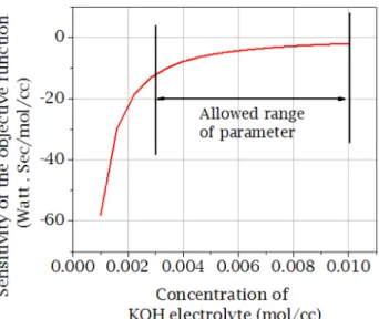
A similar trend is observed for the model parameter ce. Figure 8 shows the variation of the sensitivity of the objective function with respect to the concentration of the electrolyte,
Figure 8. The variation of the sensitivity of Edischarge with respect to the
model parameter ce
The sensitivity of the objective function with respect to ce is found to be an order of magnitude greater than that found in figure 6. This is partly due to the differences in the amount of influences the model parameters have on the objective function
and partly due to the fact that these quantities are absolute sensitivity values and they represent changes in the objective function for unit changes in the model parameters.
Figure 9. The values of the objective function for different values of the parameter ce
The optimization results in the set of values for the selected model parameters as shown in equation (30), where the symbols , , and represent the optimized values. The corresponding value of the objective function is given in equation (31). For the sake of comparison, the initial value of the objective function is also shown in equation (31).
(30)
(31)
Figure 10. Variation of the objective function with different values of the model parameter Apos
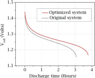
The set of model parameters affect the discharge curve in a few ways. First it increases the total time of discharge from an initial 3.07 hours to an optimized 3.78 hours. It also increases the average value of the quantity vcell, which results in an overall increase in the total amount of energy harnessed from the system. These are clearly illustrated in figure 11, which shows the discharge curves for the original and optimized system.
As mentioned before, a source of possible error for this formulation is the expression shown in equation (28). For this example, the results were numerically tested using a finite difference formulation.
For the model parameters Aneg and ce the effects of ignoring the changes in the limits of integration were found to be numerically negligible. For the parameter Apos however, the effect was found to be more prominent. This was caused by the influence of the positive electrode towards the increase of the discharge time. However, the overall effect of this approximation was determined to be insignificant for the outcome of the optimization process.
Figure 11. Discharge curves for the optimized and the original system
Conclusions
In an attempt to capture a part of the underlying physics governing a Ni-MH battery, a math-based model is presented in this paper. The model is based on the actual electro-chemical process and it captures the charging discharging characteristics of a typical Ni-MH battery along with the effects of side reactions taking place at the electrodes. The charging-discharging characteristics were found to be consistent with experimental data. The physics-based approach ensures a direct access to the actual physical parameters of the battery. The model has been implemented in MapleSim as a custom component and as such can be used as a sub-system to model various complicated system like hybrid vehicles.
Analytical sensitivity analysis was performed on the model to illustrate the application of sensitivity information for design optimization. An optimization problem was set up to maximize the total amount of energy that can be extracted from a battery at a state of full charge.
This study has used Maple for the simulations and analyses, due to its symbolic capabilities. This model is completely analytical and takes full advantage of symbolic formulation, which in turn permits the use of analytical methods for sensitivity analysis and related studies. Direct differentiation method is being used to obtain sensitivity information from the governing equations.
Currently the model does not account for some features of Ni-MH batteries. These batteries tend to self-discharge at a rate higher than that of alkaline batteries. Each charging / discharging cycle sheds active material from the electrodes, resulting in a decrease in the available energy. Also the internal resistance increases gradually over time, eventually making the battery unusable. These features limit the usable life of a battery. Future work on this subject would be focused on modeling these degradation phenomena. This model is expected to be acceptably accurate for low and moderate charging discharging currents. Temporal changes like change in concentration and potential within the electrodes are ignored in this model. Also the model presented here does not account for the hysteresis phenomenon.
One important shortcoming of this model is the assumption of a constant value of the internal resistance. The internal resistance of a NiMH battery is a complex quantity that is affected by many factors like battery temperature, battery geometry, state of charge, even shelf time [11, 10].
Under normal simulations, this assumption of constant value of internal resistance does not cause any inaccuracies. However when a design optimization is attempted to adjust the model parameters that affect the internal resistance, the deviations become more and more apparent. Therefore, to ensure that the model is suitable for optimization, proper modeling of the internal resistance is essential.
The use of MapleSim to model the effect of varying internal resistance is a current topic of research. As a multi-domain modeling tool, MapleSim is suitable for the use of experimental data in conjunction with the existing analytical model of the battery. Future research efforts will be directed toward experimental validation of the model of the internal resistance.
Acknowledgments
Financial support for this work has been provided by the Natural Sciences and Engineering Research Council of Canada (NSERC), Toyota, and Maplesoft.
References
1. Chen, M. and Rinćo Mora, G.A., “Accurate electrical battery model capable of predicting runtime and I-V performance”, IEEE Trans, On Energy Conversion, Vol. 21, No. 2, pp.504-511, 2006.
2. Paxton, B. and Newman, J., “Modeling of nickel-metal hydride batteries”, Journal of Electrochemical Society, Vol. 144, No. 11, pp. 3818-3831, 1997.
3. Newman, J. and Thomas-Alyea, K. E., “Electrochemical Systems”, 3rd ed, John Wiley & Sons Inc., 2004.
4. Albertus, P., Christensen, J., and Newman, J., “Modeling side reactions and non-isothermal effects in nickel metal-hydride batteries”, Journal of the Electrochemical Society, Vol. 155, No. 1, pp. A48-A60, 2008.
5. Wu, B., Mohammed, M., Brigham, D., Elder, R., and White, R.E., “A non-isothermal model of a nickel-metal hydride cell”, Journal of Power Sources, Vol. 101, No. 2, pp.149-157, 2001.
6. Salameh, Z.M., Casacca, M.A., and Lynch, W.A., “A mathematical model of lead-acid batteries”, IEEE
Transactions on Energy Conversions, Vol. 7, No. 1, pp. 93-98, 1992.
7. Dao, T. S., Seaman, A. and McPhee, J., Mathematics-Based Modeling of a Series-Hybrid Electric Vehicle”, Proc. of the 5th Asian Conference on Multi-body Dynamics, Kyoto, Japan, August 2010
8. Seaman, A. N. and McPhee, J., “Symbolic Math-Based Battery Modeling for Electric Vehicle simulation”. Proceedings of the ASME 2010 International Design Engineering Technical Conferences & Computers and Information in Engineering Conference, August 2010, Montreal, Canada.
9. Banerjee, J., Dao, T., and McPhee, J., “Mathematical Modeling and Symbolic Sensitivity Analysis of Ni-MH Batteries,” SAE Technical Paper 2011-01-1371, 2011, doi:10.4271/2011-01-1371.
10. Battery Internal Resistance, Energizer Technical Bulletin, Version 1.1.0, December 2005.
11. Kopera, J. J. C., Inside the Nickel Metal Hydride Battery - COBASYS Product Review, June 25th 2004.
The Engineering Meetings Board has approved this paper for publication. It has successfully completed SAE’s peer review process under the supervision of the session organizer. The process requires a minimum of three (3) reviews by industry experts.
All rights reserved. No part of this publication may be reproduced, stored in a retrieval system, or transmitted, in any form or by any means, electronic, mechanical, photocopying, recording, or otherwise, without the prior written permission of SAE International.
Positions and opinions advanced in this paper are those of the author(s) and not necessarily those of SAE International. The author is solely responsible for the content of the paper.
ISSN 0148-7191