Zurich Open Repository and Archive University of Zurich Main Library Strickhofstrasse 39 CH-8057 Zurich www.zora.uzh.ch Year: 2018
Subgroup identification in dose-finding trials via model-based recursive partitioning
Thomas, Marius ; Bornkamp, Björn ; Seibold, Heidi
Abstract: An important task in early‐phase drug development is to identify patients, which respond better or worse to an experimental treatment. While a variety of different subgroup identification methods have been developed for the situation of randomized clinical trials that study an experimental treatment and control, much less work has been done in the situation when patients are randomized to different dose groups. In this article, we propose new strategies to perform subgroup analyses in dose‐finding trials and discuss the challenges, which arise in this new setting. We consider model‐based recursive partitioning, which has recently been applied to subgroup identification in 2‐arm trials, as a promising method to tackle these challenges and assess its viability using a real trial example and simulations. Our results show that model‐based recursive partitioning can be used to identify subgroups of patients with different dose‐response curves and improves estimation of treatment effects and minimum effective doses compared to models ignoring possible subgroups, when heterogeneity among patients is present.
DOI: https://doi.org/10.1002/sim.7594
Posted at the Zurich Open Repository and Archive, University of Zurich ZORA URL: https://doi.org/10.5167/uzh-151171
Journal Article Accepted Version
Originally published at:
Thomas, Marius; Bornkamp, Björn; Seibold, Heidi (2018). Subgroup identification in dose-finding trials via model-based recursive partitioning. Statistics in Medicine, 37(10):1608-1624.
Subgroup identification in dose-finding trials via
model-based recursive partitioning
Marius Thomas
Novartis Pharma AG, Basel, Switzerland
Bj¨orn Bornkamp
Novartis Pharma AG, Basel, Switzerland
Heidi Seibold
University of Zurich, Zurich, Switzerland
Abstract
An important task in early phase drug development is to identify patients, which respond better or worse to an experimental treatment. While a variety of different subgroup identi-fication methods have been developed for the situation of trials that study an experimental treatment and control, much less work has been done in the situation when patients are randomized to different dose groups. In this article we propose new strategies to perform subgroup analyses in dose-finding trials and discuss the challenges, which arise in this new setting. We consider model-based recursive partitioning, which has recently been applied to subgroup identification in two arm trials, as a promising method to tackle these challenges and assess its viability using a real trial example and simulations. Our results show that model-based recursive partitioning can be used to identify subgroups of patients with differ-ent dose-response curves and improves estimation of treatmdiffer-ent effects and minimum effective doses, when heterogeneity among patients is present.
Keywords: personalized medicine; regression trees; non-linear models; dose estimation
This is the pre-peer reviewed version of the following article:
Thomas, M., Bornkamp, B., & Seibold, H. (2018). Subgroup identification in dose-finding trials via
model-based recursive partitioning. Statistics in medicine, 37(10), 1608-1624,
which has been published in final form at https://doi.org/10.1002/sim.7594. This article may be
used for non-commercial purposes in accordance with Wiley Terms and Conditions for Self-Archiving.
1
Introduction
The identification of subgroups (defined in terms of baseline covariates) with a modified response to a treatment is an important, but also challenging task in drug development. Firstly the identi-fication task itself is not trivial: Covariates may act on the response independent of any treatment (prognostic covariates), but usually one is interested in covariates modifying the response to the specific treatment administered (predictive covariates). In addition, the treatment effect may be defined in terms of a non-trivial function of the covariates. Further statistical issues include mul-tiplicity, bias in treatment effect estimates in selected subgroups (due to the selection) and sample sizes that are typically too low to detect relevant differences between subgroups. A high-level overview of the involved statistical challenges but also opportunities is given in [1].
The development of computational and statistical tools to identify subgroups/covariates leading to a differential response has been a major focus of statistical research in recent years. Due to their ability to handle high-order interactions and their good interpretability, many of the proposed approaches employ tree-based partitionings of the overall trial data [2, 3, 4, 5, 6]. Other statistical approaches to the problem include Bayesian models [7] and penalized regression coupled with a transformation of the covariates [8]. A recent overview paper on the topic of subgroup identification is [9].
Most of these methods have been developed in the context of clinical trials that compare a new treatment against a control. However studies with more than one dose of the active treatment are also common in clinical trials conducted in late-stage development. This is obviously true for Phase II dose-finding trials (see [10, 11] for an overview), but also in Phase III trials sometimes two or three doses are studied. When patients are administered different doses of the new treatment and a subgroup search is performed, this search has to be adjusted for the fact that patients received different doses: One patient might respond better compared to another patient because they differ in the dose received but not because of their differing baseline characteristics.
One way to approach this problem is to assume a functional relationship between dose and response to account for dose, but allow that this relationship can differ across subgroups. One can for example assume a the Emax function, a standard parametric model in dose-response analyses [10, 12], which leads to a function non-linear in its parameters. Alternatively a spline function might be used. Another alternative would be to use a model that just describes the treatment
effect at the observed doses and makes no assumptions about the functional replationship. The idea in all three cases would then be that within each subgroup the same type of model is fitted, but the model parameters would vary between subgroups.
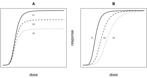
In the setting of dose-response analyses the consequences of finding subgroups is different than in standard subgroup analyses, because subgroups might differ not only in their treatment effect but more generally in terms of the shape of the dose-response curve. One might, for example, identify subgroups that have an increased or decreased treatment effect (such as in Figure 1A). But one might also identify subgroups requiring a different dose to achieve a desired treatment effect (such as in Figure 1B).
A dose S1 S2 S3 B dose response S1 S2 S3
Figure 1: Example of different dose-response shapes in three exemplary subgroups S1-S3. A shows subgroups with different maximum treatment effects, B shows an example of subgroups of patients potentially requiring different doses,
In this paper we want to propose the use of model-based recursive partitioning in this setting. This approach has originally been proposed in [13] and applied to subgroup analyses for two-armed trials in [14]. This algorithm splits the overall trial population recursively into subgroups (defined by baseline covariates), so that each group has a homogeneous dose-response relationship. The advantages of this approach compared to other approaches for recursive partitioning are that (i) it is easily adaptable to different statistical models (such as different endpoint distributions and also nonlinear models), (ii) it contains an easily interpretable stopping criterion to control the
complexity of the tree and (iii) allows to restrict the splitting to specific model parameters, which can be helpful to distinguish between prognostic and predictive effects. In addition the methodology is implemented in the publicly available R package partykit [15]. The purpose of this paper is to investigate the suitability of this method in the context of dose-finding trials.
The paper is structured as follows: In the next section we will introduce a motivating example dose-finding study. In Section 3 we will first discuss the considered dose-response models and then introduce model based recursive partitioning in this context. Section 4 contains a simulation study evaluating the properties of the proposed method and comparing different models. In Section 5 the trial example will be revisited and analysed to illustrate the methodology on a concrete data example. Conclusions and some discussion are presented in Section 6.
2
A motivating example
Exploratory subgroup analyses are performed in many stages of clinical drug development. In Phase II these analyses are performed to identify whether any and/or which baseline covariates modify the treatment effect. The result of these analyses will inform decisions regarding the further development of the drug, for example how subsequent clinical trials are designed.
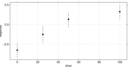
As an example we consider data from a dose-finding trial conducted to assess the efficacy of a new treatment for an inflammatory disease. For reasons of confidentiality all variable names are non-descriptive and all continuous variables have been rescaled to have mean 0 and standard deviation 1. We have complete data from 270 patients, which were distributed across 4 arms, receiving either a placebo (n = 75) or the new drug at dose levels 25 (n= 54), 50 (n = 62) and 100 (n= 79). The primary endpoint is the change from baseline in a continuous variable. Additionally baseline measurements of 10 covariates – 6 of which are categorical and 4 of which are continuous – are available for each patient.
The mean responses at the dose levels in the trials along with the confidence intervals are shown in Figure 2, which suggest a clear dose-response effect. Still there is interest in further investigation of whether there is a subgroup with differential treatment effect. This analysis and its results are discussed in Section 5, using the methodology developed in Section 3.
dose response −0.5 0.0 0.5 0 20 40 60 80 100 ● ● ● ●
Figure 2: Mean responses and 90%-confidence intervals for the dose-finding trial example.
3
Statistical methodology
In this section we will first introduce the dose-response models we consider. Even though we focus on normally distributed endpoints in the rest of the article, we will introduce the models in a generalized form, which also allows for other commonly encountered outcome types in clinical trials, such as binary, count or time-to event data.
In the second part of this section we will then introduce the model-based recursive partitioning method in the context of dose-response modeling. A more detailed discussion of the algorithm can be found in [13].
3.1
Model specification
We consider the situation of a clinical trial with n patients, that receive doses d1, ..., dn of a new
treatment at l dose levels, so that di ∈ {d˜1, ...,dl˜}, where the lowest level is a placebo ˜d1 = 0.
We observe responses y1, ..., yn, which can be related either to efficacy or safety of the drug in
question. Typically a small set of additional baseline covariatesxi of dimensionK for each patient
i, are measured and adjusted for in the analysis, examples are the baseline value of the outcome (if change from baseline is used) or covariates like region, center or other stratification variables.
from the space of the response variable to R and ηi is a (possibly non-linear) predictor such that
ηi =β0+ ∆(di,θ) +γ
′
xi. (1)
β0 is an intercept describing the response under placebo and ∆(di,θ) is a dose-response function
with parameter vectorθ (with ∆(0,θ) = 0), which describes the treatment effect in dependence of the dose level. Additional covariate main effects are modeled in γ.
In total we obtain a model m((y,d,X),ϕ) with y = (y1, ..., yn), d = (d1, ..., dn), X =
(x1, ...,xn) and ϕ = (β0,θ,γ, σ), where σ is a nuisance parameter, as for example the standard
deviation of the response in a Gaussian GLM. An estimate forϕ can be derived as ˆ ϕ= arg min ϕ n X i=1 Ψ((yi, di,xi),ϕ),
by minimizing the objective function Ψ corresponding to modelm, for example the log-likelihood. In what follows we will only consider normally distributed outcomes, so that this reduces to the residual sum of squares in our setting. Finding the minimum above is equivalent to solving
n X i=1 ∂Ψ((yi, di,xi),ϕ) ∂ϕ = n X i=1 ψ((yi, di,xi),ϕ) = 0,
whereψ is the score function.
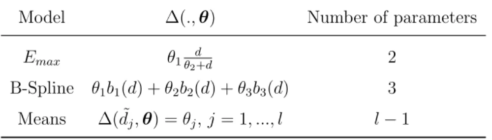
We will now give an overview over the different functional forms of ∆, which will be used to model dose-response relationships in the remainder of this article. These forms of ∆ contain non-linear and non-linear models and show varying degrees of flexibility in regards to the dose-response shapes, which they can fit. Table 1 shows a summary.
Table 1: Functional forms of ∆ used to model dose-response. b1, b2, b3 denote basis functions of a
B-spline with degree 2 and one inner knot at the median of the dose levels.
Model ∆(.,θ) Number of parameters
Emax θ1θ2d+d 2
B-Spline θ1b1(d) +θ2b2(d) +θ3b3(d) 3
Means ∆( ˜dj,θ) =θj, j = 1, ..., l l−1
The Emax model is commonly used to model plateauing, monotonic dose-response functions [10]. It has been shown to be adequate in a wide variety of real dose-response situations, see [12],
and is, as many other dose-response models, non-linear in its parameters. It can be derived from pharmacological principles [16] and its parameters have a direct interpretation, as θ1 represents
the maximum treatment effect, which is reached as the dose goes to infinity, and θ2 represents the
dose required to receive 50% of this maximum effect.
To relax the parametric assumptions, we also consider a spline model, which is linear in the parameters and uses transformations of the dose variable as the independent variable in the model. As only a limited number of dose-levels is typically used in dose-finding trials, we use quadratic B-splines with only one knot at the median of the active dose levels. This model can fit a large number of possible dose-response shapes well, but requires the estimation of one more parameter than the Emax model.
The last “Means” model estimates the treatment effects independently, without assuming a relationship among the doses. It does not make any assumptions about the underlying dose-response relationship and treats the different dose levels as independent treatments. This allows for additional flexibility in the possible dose-response relationship, but can possibly overfit the data and lead to biologically implausible estimated dose-response relationships. In addition this model does not allow to predict the dose-response effect beyond the actually observed doses. An interpolation method, for example using splines, is required to obtain predicted responses for dose levels which lie between the observed dose levels.
3.2
Model-based recursive partitioning
Primary, pre-specified analyses of clinical trials typically assume that the treatment effect is homo-geneous across the population studied. Baseline covariates (as in Equation 1) are typically included only if they are considered important already at the design stage of the trial. Nevertheless addi-tional baseline covariates Z might have been measured and it is of interest to evaluate the effect that these might have on the dose-response model.
This can be achieved with model-based recursive partitioning (ormob for short). This approach applies a parametric model and allows for the parameters to depend on certain baseline covariates (e.g. biomarkers) Z. We can thus rewrite the model as m((y,d,X),ϕ(Z)). This is achieved by estimating separate models for different subgroups. These subgroups are found through an algorithm, which recursively tries to detect, if there are covariate effects on the parameters of model m. If covariate effects are detected, the algorithm will split the patients into subgroups
using these covariates. Then in each of these subgroups models are estimated separately.
To detect covariate effects the model-based recursive partitioning algorithm makes use of tests for parameter instability in model m. Parameter instability can be discovered by testing for independence between the partial scores and covariatesz(1), . . . ,z(J), i.e.
ψϕp((y,d,X),ϕˆ) ⊥ z
(j), j = 1, . . . , J, p= 1, . . . , P (2)
with J being the number of partitioning covariates andP the number of model parameters. The partial score ψϕp is the partial derivative of the objective function with respect to the model parameterϕp respectively. For a detailed discussion of the algorithm and the instability tests used, see [13] and [17].
If the overall null hypothesis of no instability (for any of the parameters) is not rejected, we assume no (further) subgroups. If it is rejected, the variable corresponding to the smallestp-value is chosen as split variable. The subgroups are formed based on this split variable using a binary split. If there are multiple possible splits over the variable, the split, which minimizes the objective function of the model in the two resulting subgroups is chosen. Then new models are estimated in each subgroup and the parameters of each model are again tested for instability. New subgroups are formed until the overall null hypothesis can no longer be rejected or other stop criteria come into effect (for example the minimum subgroup size is reached).
In each step of the algorithm (for each split)J×P null hypotheses (see Equation 2) are tested. To adjust for the fact that multiple tests are performed a Bonferroni correction is used.
In addition one might be especially interested in specific parameters. For example in the dose-response models the effects γ of baseline covariates and nuisance parameters σ may only be of secondary interest. Then it is possible to restrict the instability tests on partial scores with respect to parameters β0 and θ. For the subgroup analyses we consider here, one might even go further
and restrict the splitting only to θ, since only these parameters impact the treatment effect.
4
Simulation study
This section will show the results of simulations to evaluate the performance of the previously described methods in simulation scenarios. Our simulation scenarios aim to represent the situation of a Phase II dose-finding trial, for which exploratory subgroup analyses are regularly conducted.
The main characteristics of the study we simulate, e.g. the general form of the dose-response curve, the dose levels used and the standard error are based on a study to investigate the efficacy and safety of glycopyrronium bromide in COPD patients. The summary statistics from this study can be found onclinicaltrials.gov under NCT00501852.
We simulate clinical trials with n= 250 patients, which are equally distributed across 4 active doses (12.5, 25, 50, 100) and a placebo, resulting in 5 dose levels in total with 50 patients each. We generate a vector of baseline covariates for each patient ias zi ∼N(0,I10). We generate data
from an Emax model of the form
yi ∼N(µi, σ2) i.i.d, µi =β0(zi) +θ1(zi) di θ2(zi) +d for i=1,...n, (3)
For this model the parameters describing placebo response (β0), maximum effect (θ1) and the dose
giving 50% of the response (θ2) depend on a patient’s baseline covariates. The ratio of effect size
to noise can be controlled through σ. Unless explicitly stated otherwise σ is always set to 0.12 in the following simulations.
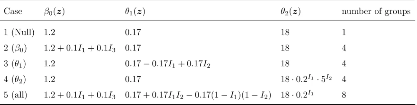
Table 2: Base cases for simulation study. Here Ij =I(z(j) >0). The rightmost column gives the
number of groups, e.g. the size of a partition needed to achieve completely homogeneous groups of patients with regards to the parameters of the model.
Case β0(z) θ1(z) θ2(z) number of groups
1 (Null) 1.2 0.17 18 1
2 (β0) 1.2 + 0.1I1+ 0.1I3 0.17 18 4
3 (θ1) 1.2 0.17−0.17I1+ 0.17I2 18 4
4 (θ2) 1.2 0.17 18·0.2I1·5I2 4
5 (all) 1.2 + 0.1I1+ 0.1I3 0.17 + 0.17I1I2−0.17(1−I1)(1−I2) 18·0.2I1 8
We consider five cases for our simulation study, which include a null case with no covariate effects, three cases with covariate effects on only one of the parameters of the model and one case with covariate effects on all parameters. For details see Table 2. With the 5 considered cases we simulate scenarios, where there are:
2 subgroups with differences in placebo response (change in β0);
3 subgroups with a doubled treatment effect, while others have none (change in θ1);
4 subgroups, for which the dose-response curve is very steep, and plateaus near the lower end of the dose range, while for others the curve is very shallow and the plateau is not reached at the maximum dose (change in θ2);
5 a combination of 2-4.
The following simulations can be divided into two parts with different objectives. The first part tries to evaluate how well the mob procedure resolves the bias-variance trade-off in data partitioning: A global model fitted to all data might be biased, but will have smaller variability in parameter estimates, compared to a model that uses the true partitions. Using the true partitions will lead to unbiased parameter estimates but larger variability in parameter estimates (due to smaller sample size in each subgroup). The mob procedure can be considered as an adaptive procedure, as it decides on the model complexity adaptively (i.e. it might also fit a global model if no split is selected in the first step). These first simulations therefore comparemob to these two extreme cases (global model and the model using the true partitions). Their results are discussed in Section 4.1.
The second part of the simulations is concerned with evaluating the performance of the algo-rithm in regards to subgroup analyses. In these simulations, which are discussed in Section 4.2, the subgroup identification and estimation performance is evaluated.
We use the function mob in the R package partykit together with our own user-defined fitting function, which can be found in the appendix. We focus on the case of a normally distributed response variable and include no additional baseline covariates in the models. The trees use models of the form
yi ∼N(µi, σ2) i.i.d, µi =β0+ ∆(di,θ) for i=1,...,n,
where ∆ has one of the functional forms shown in Table 1, the corresponding methods will be called mobEmax, mobSpline and mobMeans in what follows. We will use the algorithm described in 3.2 to detect instabilities over the partitioning variables z. Two different approaches for selection of
variables for the splits are used. In one approach instabilities in bothβ0 and θ are tested (denoted
as “unrestricted” in what follows), in the other testing is restricted to the parameters inθ, which affect the dose-response function (denoted as “restricted” in what follows). This is implemented via the parm argument in mob.
As additional arguments for themob function we use control parameters ofalpha = 0.1, minsize = 20 and maxdepth = 4, which respectively control the significance level used for the instability tests at each split, the minimum size of the subgroups and the maximum depth of the tree.
4.1
Improvement in model fit
Partitioning the data when covariate effects are present should improve the model fit on independent test data, compared to a global model. Evaluating if there is a benefit in partitioning the data and if the partitioning algorithm can reliably find these partitions should be the first step, when assessing the properties of the method. For this purpose we generate training sets of size n= 250 and test sets of sizen = 10000 from the model in Equation (3). We use the training set to fit the model and calculate the log-likelihood of the test set data under the fitted model. We compare three models: the global model, which fits one model for all patients, the model partitioned by
mob and a model fit on the true partition.
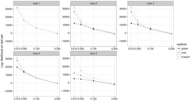
Figure 3 shows the median of the log-likelihood on the test sets over 5000 simulations for the cases in Table 2 depending on standard deviationsσ, when usingEmax models. The plot visualizes the trade-off between bias and variance. For small σ partitioning the data clearly leads to a better model fit, since a larger fraction of the variance is explained by covariate effects on the model parameters rather than the error variance and refraining from partitioning the data leads to biased inference for some patients. As σ increases, the benefit of partitioning the data decreases. Partitioning the data and fitting models separately on a small group of patients leads to parameter estimates that are too variable, when the data are noisy (even when using the true partition).
As mob adaptively decides if the data should be partitioned the model fit on the test set is usually somewhere between the global model and using the true partition (which is of course unknown in reality). The only exception for this seem to be the scenarios with σ = 0.125 and
σ = 0.25 and under case 2, 3 and 5, where mob sometimes shows a slightly worse fit than both the global model and the model using the true partition. In the scenarios with smaller σ mob
● ● ● ● ● ● ● ● ● ● ● ● ● ● ● ● ● ● ● ● ● ● ● ● ● ● ● ● ● ● ● ● ● ● ● ● ● ● ● ● ● ● ● ● ● ● ● ● ● ● ● ● ● ● ● ● ● ● ● ● ● ● ● ● ● ● ● ● ● ● ● ● ● ● ● ● ● ● ● ● ● ● ● ● ● ● ● ● ● ● ● ● ● ● ● ● ● ● ● ● ● ● ● ● ● ● ● ● ● ● ● ● ● ● ● ● ● ● ● ● ● ● ● ● ● ● ● ● ● ● ● ● ● ● ● ● ● ● ● ● ● ● ● ● ● ● ● ● ● ● ● ● ● ● ● ● ● ● ● ● ● ● ● ● ● ● ● ● ● ● ● ● ● ● ● ● ● ● ● ● ● ● ● ● ● ● ● ● ● ● ● ● ● ● ● ● ● ● ● ● ● ● ● ● ● ● ● ● ● ● ● ● ● ● ● ● ● ● ● ● ● ● ● ● ● ● ● ● ● ● ● ● ● ● ● ● ● ● ● ● ● ● ● ● ● ● ● ● ● ● ● ● ● ● ● ● ● ● ● ● ● ● ● ● ● ● ● ● ● ● ● ● ● ● ● ● ● ● ● ● ● ● ● ● ● ● ● ● ● ● ● ● ● ● ● ● ● ● ● ● ● ● ● ● ● ● ● ● ● ● ● ● ● ● ● ● ● ● ● ● ● ● ● ● ● ● ● ● ● ● ● ● ● ● ● ● ● ● ● ● ● ● ● ● ● ● ● ● ● ● ● ● ● ● ● ● ● ● ● ● ● ● ● ● ● ● ● ● ● ● ● ● ● ● ● ● ● ● ● ● ● ● ● ● ● ● ● ● ● ● ● ● ● ● ● ● ● ● ● ● ● ● ● ● ● ● ● ● ● ● ● ● ● ● ● ● ● ● ● ● ● ● ● ● ● ● ● ● ● ● ● ● ● ● ● ● ● ● ● ● ● ● ● ● ● ● ● ● ● ● ● ● ● ● ● ● ● ● ● ● ● ● ● ● ● ● ● ● ● ● ● ● ● ● ● ● ● ● ● ● ● ● ● ● ● ● ● ● ● ● ● ● ● ● ● ● ● ● ● ● ● ● ● ● ● ● ● ● ● ● ● ● ● ● ● ● ● ● ● ● ● ● ● ● ● ● ● ● ● ● ● ● ● ● ● ● ● ● ● ● ● ● ● ● ● ● ● ● ● ● ● ● ● ● ● ● ● ● ● ● ● ● ● ● ● ● ● ● ● ● ● ● ● ● ● ● ● ● ● ● ● ● ● ● ● ● ● ● ● ● ● ● ● ● ● ● ● ● ● ●
case 1 case 2 case 3
case 4 case 5 −10000 0 10000 20000 30000 −10000 0 10000 20000 30000 −10000 0 10000 20000 30000 −10000 0 10000 20000 30000 −10000 0 10000 20000 30000 0.010 0.050 0.125 0.250 0.010 0.050 0.125 0.250 0.010 0.050 0.125 0.250 0.010 0.050 0.125 0.250 0.010 0.050 0.125 0.250 σ Log−lik
elihood on test set
method ● global
mob truepart
Figure 3: Median log-likelihood of test set data of sizen = 10000 underEmaxmodels fit on training data of size n = 250 for all simulation cases and varying standard deviations σ. Global refers to one model fit for all patients, mob to model-based recursive partitioning and truepart to models fit on the true partition.
partitioning the data and therefore shows a similar fit as the global model.
4.2
Subgroup identification and estimation of dose-response curve
In this section performance metrics relevant for subgroup analyses will be discussed in more detail.
Identification of correct covariates Identifying the covariates, that interact with the
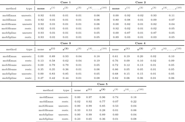
treat-ment is a main interest of subgroup analyses. Based on these covariates subgroups of patients with differential responses to the treatment can be defined. In this section we will therefore discuss the results of simulations, which aim to evaluate the capability of the method to partition over the correct baseline covariates. Additionally we investigate the rate of false positive discoveries, when there are no interactions between covariates and treatment. For these purposes we track the structure of the tree, e.g. for each trial simulation and each of the 10 covariates, we track if the covariate is used as a split variable in the corresponding mob tree. Table 3 shows the results averaged over 5000 simulations.
Table 3: Relative frequency of covariates appearing in the trees for differentmob models with and without restriction to treatment effect parameters over 5000 simulations. Covariates in bold are interacting with the treatment effect. z1 and z3 are prognostic for Cases 2 and 5.
Case 1 Case 2
method type none z(1) z(2) z(3) z(4), . . . , z(10) none z(1) z(2) z(3) z(4), . . . , z(10) mobEmax unrestr. 0.92 0.01 0.01 0.01 0.06 0.00 0.92 0.02 0.93 0.11 mobEmax restr. 0.92 0.01 0.01 0.01 0.06 0.80 0.08 0.01 0.09 0.07 mobMeans unrestr 0.92 0.01 0.01 0.01 0.06 0.00 0.82 0.01 0.82 0.04 mobMeans restr. 0.92 0.01 0.01 0.01 0.05 0.92 0.02 0.01 0.02 0.05 mobSpline unrestr 0.93 0.01 0.01 0.01 0.05 0.00 0.87 0.01 0.87 0.05 mobSpline restr. 0.93 0.01 0.01 0.01 0.05 0.89 0.03 0.01 0.03 0.05 Case 3 Case 4
method type none z(1) z(2) z(3) z(4), . . . , z(10) none z(1) z(2) z(3) z(4), . . . , z(10) mobEmax unrestr. 0.00 0.89 0.93 0.04 0.18 0.61 0.19 0.20 0.02 0.10 mobEmax restr. 0.13 0.58 0.62 0.04 0.19 0.76 0.09 0.10 0.02 0.09 mobMeans unrestr. 0.00 0.79 0.79 0.01 0.05 0.72 0.12 0.13 0.01 0.05 mobMeans restr. 0.35 0.35 0.36 0.01 0.06 0.86 0.05 0.05 0.01 0.05 mobSpline unrestr. 0.00 0.83 0.85 0.01 0.05 0.68 0.15 0.15 0.01 0.05 mobSpline restr. 0.27 0.42 0.44 0.01 0.08 0.82 0.06 0.06 0.01 0.06 Case 5
method type none z(1) z(2) z(3) z(4), . . . , z(10) mobEmax unrestr. 0.00 0.97 0.96 0.74 0.18 mobEmax restr. 0.02 0.92 0.77 0.07 0.22 mobMeans unrestr. 0.00 0.99 0.85 0.53 0.04 mobMeans restr. 0.33 0.53 0.28 0.01 0.06 mobSpline unrestr. 0.00 0.99 0.89 0.60 0.04 mobSpline restr. 0.23 0.65 0.36 0.01 0.08
In case 1 and 2 there are no covariates interacting with the treatment. For case 1, where there are no covariate effects whatsoever, all models do not partition the data in more than 90% of cases and thus control the type I error at the nominal level. In case 2 restricting the partitioning to the treatment effect parameters makes a big difference. If the partitioning is restricted in this way there is often no partitioning of the data, but still more often than in case 1. When there is no restriction, the correct covariatesz(1) and z(3) are found with high frequency.
Cases 3-5 include covariate interactions with the treatment. In cases 3 and 5 the method picks up the predictive effects of z(1) and z(2) well. If partitioning is not restricted then the purely prognostic covariate z(3) is also correctly included. In case 4 finding predictive effects on θ
2 seems
to be more challenging. None of the methods reliably partition over the predictive covariates z(1)
and z(2). These covariates do appear in more trees than z(3), which is just noise in this case, but
more than 50% of the time a global model is fitted.
mobSpline and mobMeans seem to be more greatly affected by restricting partitioning. They both partition less often.
Estimating quantities of interest In dose-finding trials two important quantities of interest
are the treatment effect at specific dose levels, as well as the minimum effective dose (MED), which is the smallest dose required to achieve a relevant treatment effect over placebo. Being able to estimate both of these precisely is therefore of great importance for a method used in these settings. In the situation we consider for this article this is especially challenging, since the patient populations can be heterogeneous with regards to both of these quantities.
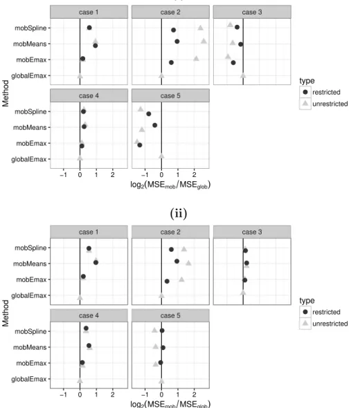
To evaluate the treatment effect estimation of our methods we estimate the treatment effect individually for each patient at a sequence of dose levels from 1 to 100 using increments of 1. We average the squared error of these 100 estimates for each patient and then average over all patients to obtain the MSE of the individual treatment effect estimates. We compare these estimates as obtained throughmob with the estimates from a globalEmaxmodel fit for all patients. We consider
σ= 0.12 andσ = 0.24 as standard deviations, where the latter setting simulates a scenario, where any effects are small in relation to the error variance and therefore harder to detect.
Figure 4 shows the MSE ofmob with different dose-response models relative to the globalEmax
model. In cases, where covariates do not affect the treatment effect (cases 1 and 2) mob methods increase the MSE of treatment effect estimates, since the global Emax model is the better suited
model in these situations. When using mob in combination with the Emax model, the increase is very small in case 1, since mob rarely partitions the data (see Section 4.2). For case 2 the effect of restricting splitting to treatment effect parameters becomes visible. Since covariate effects here are only prognostic, restricting the parameters over which to split, reduces the MSE. If splitting happens unrestricted, MSEs are more than quadrupled in some situations, compared to the global
Emax model.
In Cases 3 and 5 the advantages of partitioning the data become clearly visible. Here using
mob methods leads to a clear reduction of the MSEs for σ = 0.12, which are in some situations more than halved. For the largerσ reduction can only be seen in Case 5, while in Case 3 the MSEs are similar to those under the global model. Restriction of splitting on parameters relevant for the treatment effect weaken the observed improvements somewhat.
(i) ● ● ● ● ● ● ● ● ● ● ● ● ● ● ●
case 1 case 2 case 3
case 4 case 5 globalEmax mobEmax mobMeans mobSpline globalEmax mobEmax mobMeans mobSpline −1 0 1 2 −1 0 1 2
log2(MSEmob MSEglob)
Method type ● restricted unrestricted (ii) ● ● ● ● ● ● ● ● ● ● ● ● ● ● ●
case 1 case 2 case 3
case 4 case 5 globalEmax mobEmax mobMeans mobSpline globalEmax mobEmax mobMeans mobSpline −1 0 1 2 −1 0 1 2
log2(MSEmob MSEglob)
Method
type
● restricted unrestricted
Figure 4: Reduction of MSE for individual treatment effect estimation of the mob methods com-pared to a global Emax model as log2(M SEM SEglobalEmaxmob ) over 5000 simulations with residual standard
deviation ofσ = 0.12 (i) and σ = 0.24 (ii).
methods and the global model. As also shown in the results in Section 4.2, covariate effects on the
θ2 parameter, which lead to steeper or shallower curves seem to be much harder to identify.
Comparing the different mob dose-response models to each other, the correct Emax model
performs the best, having the smallest MSEs of all mob methods in most scenarios, as expected as this is the true model. The remaining models, however, show similar performance with slightly worse MSE in cases 3 and 5, with the mobSpline typically being better than mobMeans.
in areas of the dose-response curve, where the curve is very steep. In these areas small deviations of the dose can lead to large changes in response. We therefore assume that there is an interval of doses around the true MED, which are all acceptable doses to pick and the width of this interval depends on the steepness of the curve. For our simulations we assume, that the minimum relevant effect size is 0.1, but consider all dosesd for which ∆(d)∈[0.08,0.12] as acceptable choices for the MED. For each simulated trial our metric is 1, if the estimated MED is in this dose range and 0 otherwise. We then average this binary metric to receive a percentage of correctly estimated MEDs over all simulated trials. The results are displayed in Figure 5.
(i) ● ● ● ● ● ● ● ● ● ● ● ● ● ● ●
case 1 case 2 case 3
case 4 case 5 globalEmax mobEmax mobAncova mobSpline globalEmax mobEmax mobAncova mobSpline 0.0 0.2 0.4 0.6 0.0 0.2 0.4 0.6
Percentage of correctly estimated MED
Method type ● restricted unrestricted (ii) ● ● ● ● ● ● ● ● ● ● ● ● ● ● ●
case 1 case 2 case 3
case 4 case 5 globalEmax mobEmax mobMeans mobSpline globalEmax mobEmax mobMeans mobSpline 0.0 0.2 0.4 0.6 0.0 0.2 0.4 0.6
Percentage of correctly estimated MED
Method
type
● restricted unrestricted
Figure 5: Percentage of correctly estimated individual MED over 5000 simulations formob methods and globalEmax model with residual standard deviation of σ= 0.12 (i) andσ = 0.24 (ii).
Results for the MED are similar to that obtained for estimating the individualized treatment effects (see Figure 5). MED estimation is improved in cases 3 and 5, when usingmob. For a global model in case 5 only about 10% of estimated MEDs are in the correct range, which shows the need for partitioning. Using mob around 30% of MED estimations are correct. In the remaining cases mob performs usually slightly worse than the global model. Case 2 again shows the effect of restricting to parameters relevant for the treatment effect. In case 2 and forσ = 0.12 unrestricted splitting has around 10 -15% fewer correctly estimated MEDs compared to restricted splitting. In general the results are qualitatively similar for both considered error variances, improvements in MED estimation can also be seen for the high variance.
When comparing dose-response models, theEmax model seems to have less of an advantage for estimating MED compared to treatment effect estimation.
5
Subgroup analysis for the example trial
We now return to the dose-finding trial described in Section 2. Using the methods discussed above we can perform an exploratory subgroup analysis. We fit an Emax model as described in Table 1 and use the mob algorithm to search for subgroups. We use control parameters of alpha = 0.1,
minsize = 20 and maxdepth = 4 and restrict the partitioning to θ to only identify subgroups,
which differ with regards to the treatment effects. The code to perform the analysis can be found in the appendix.
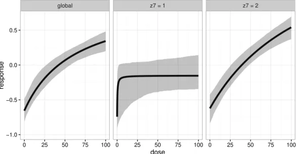
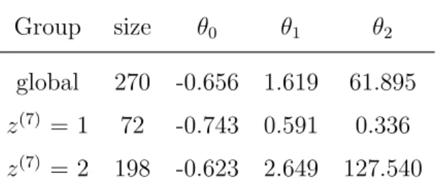
The algorithm does partition the data and finds two subgroups of size 72 and 198 based on the binary variable z(7) with an unadjusted p-value of 0.006 for the parameter instability test. Table
4 shows the parameters in the global model and the parameters of the Emax model in the two subgroups as found bymob. While the placebo effect stays roughly the same for all 3 models there are differences in θ1 and θ2, between the two subgroups. For patients withz(7) = 1 both θ1 and θ2
are estimated to be much lower than for the remaining patients.
Figure 6 shows the resulting dose-response curves in the dose range. For the patients with
z(7) = 1 a plateau is reached very quickly and roughly half of the treatment effect of the other group is achieved at the maximum dose level 100. The curve of the patients with z(7) = 2 is very
similar to the curve from the global model with slightly higher treatment effect for higher dose levels.
To assess the robustness of these findings we repeated the analysis with the other models shown in Table 1. Using these models with the same settings, we did not detect a significant parameter instability and thus the global model was fitted. Nevertheless, for all models the split with the lowest p-value was the split over covariate z(7) with unadjusted p-values 0.026 for mobMeans and 0.025 for mobSpline models. Therefore different models seem to be in unison about which covariate causes most parameter instability. In this context one should also consider the findings discussed in Section 4.2, where Emax models detected existing subgroups more often, while controlling the type I error as well as other models. Of course, in these simulations the true underlying model was alsoEmax. Nevertheless it could be the case, that models other than theEmax simply lack the power to detect this covariate effect.
There seems to be some evidence that suggests an effect of the covariate z(7) on the
dose-response shape. The strong dose-dose-response relationship observed, when fitting a global model seems to be driven by a subgroup of consisting of≈73% of the patients. The remaining patients on the other hand show a reduced treatment effect.
global z7 = 1 z7 = 2 −1.0 −0.5 0.0 0.5 0 25 50 75 100 0 25 50 75 100 0 25 50 75 100 dose response
Figure 6: Dose-response curves with 90% confidence bands for the global model and models in the two subgroups, z7 = 1 and z7 = 2.
Table 4: Parameters of theEmax model, fit globally and in the subgroups as found by mob.
Group size θ0 θ1 θ2
global 270 -0.656 1.619 61.895
z(7) = 1 72 -0.743 0.591 0.336
z(7) = 2 198 -0.623 2.649 127.540
6
Conclusions and discussion
In this article we discussed a strategy for subgroup identification in dose-finding trials based on model-based recursive partitioning.
The results depicted in Section 4.1 show that mob can be seen as an adaptive method, that implicitly tries to balance between the bias introduced through omitting potential covariate effects and the additional variance introduced by fitting models to a partitioned data-set. This is also visible in Figures 4 and 5. When using the correctEmax models (and when restricting to treatment effect parameters) using mob seems to have few disadvantages in regards to estimation. When large effects of covariates are present using mob often leads to improvements in estimation of the quantities of interest. In scenarios, where there are no covariate effects or only prognostic ones, estimation is only slightly worse than with the global model (at least when we restrict the splitting to treatment effect parameters), sincemob will often simply fit the global model in these situations (see Table 3).
From the simulation results in Section 4 it becomes clear that for sample sizes, treatment effect sizes and error variability commonly observed in clinical dose-finding trials, identification of differ-ential treatment effects is challenging. Due to the bias-variance trade-off, benefits of partitioning the data are quickly diminishing as the error variance becomes larger, as one can see in Figures 3 and 4(ii). From this perspective the type I error control is an important aspect of the method. Our simulation results depicted in Table 3 show that type I error is indeed controlled in scenarios without covariate effects. Thus, at the very least, the chance of a false positive subgroup finding, which is one concern for these types of analyses, is reduced.
The main challenge, when applying subgroup analyses in the context of dose-response trials are that many models used in this context are non-linear. Apart from the non-linearEmax model, we
therefore also considered models, which are linear in the parameters to compare their performances. Even though we only considered data generated from an Emax model, the spline model showed generally good performance, which was in most aspects only slightly worse than the Emax model. It could therefore be seen as an alternative to non-linear models, as the linearity in the parameters might be beneficial in some situations. Further research might be required to assess the method’s properties, when data is generated from other models.
One advantage of the algorithm is that it allows to restrict the partitioning over covariate effects to a specific set of parameters. In the context of subgroup analyses this can be used to distinguish between prognostic and predictive effects of covariates, where the latter are usually of greater interest. The results in Table 3 show that these restrictions can effectively be used to reduce splits over prognostic covariates. It is visible, that this also reduces the detection rate of predictive effects, which was also suggested in [14]. This setting could therefore be seen as a tuning parameter, similar to the other possible options of the algorithm like the significance level, the minimum node size and the maximum tree depth.
In this paper only normally distributed outcomes were considered for the simulations and trial example, but an extension of this method to other outcome types is possible. These extensions as well as the methods discussed in this paper can be implemented using the R package partykit.
Acknowledgements
The authors would like to thank Torsten Hothorn for helpful comments and discussions. This work was supported by funding from the European Union’s Horizon 2020 research and innovation programme under the Marie Sklodowska-Curie grant agreement No 633567 and by the Swiss State Secretariat for Education, Research and Innovation (SERI) under contract number 999754557 . The opinions expressed and arguments employed herein do not necessarily reflect the official views of the Swiss Government.
Appendix
R code for trial example
l i b r a r y ( D o s e F i n d i n g ) l i b r a r y ( p a r t y k i t ) # e m a x f i t t i n g f u n c t i o n e m a x M o b <- f u n c t i o n (y , x , start = NULL , w e i g h t s = NULL , offset = NULL ,... , estfun = FALSE , object = FALSE ){
model <- fitMod ( resp = y , dose = x , model = " emax " ,
start = start , bnds = d e f B n d s ( max ( x )) $ emax , ...) sigma <- sqrt ( model $ RSS / model $ df )
c o e f f i c i e n t s <- coef ( model ) rss <- model $ RSS
if ( estfun == 1){
n . coef <- length ( coef ( model )) param <- list ( dose = x )
param [2 : n . coef ] <- as . list ( coef ( model )[ -1]) names ( param )[2 : n . coef ] <- names ( coef ( model ))[ -1] grad <- do . call ( emaxGrad , param )
fitted . y <- p r e d i c t ( model , p r e d T y p e = " full - model " ) res <- y - fitted . y
scores <- -( res * grad ) / sigma ^2 } else { scores <- NULL } if ( object == 0) model <- NULL
return ( list ( c o e f f i c i e n t s = coef ficients , objfun = rss , estfun = scores , object = model ))
}
# m ob a n a l y s i s
p a r t v a r . names <- paste ( c o l n a m e s ( dr . dat )[1:10] , c o l l a p s e = " + " ) form <- as . f o r m u l a ( paste ( " resp ~ 0+ dose | " , p a r t v a r . names ))
parm <- 2:3 alpha <- 0.1 m i n s i z e <- 20 tree <- mob ( form ,
fit = emaxMob , c o n t r o l = mob _ c o n t r o l ( b o n f e r r o n i = TRUE , alpha = alpha , m i n s i z e = minsize , parm = parm , m a x d e p t h = 4))
References
[1] Ruberg SJ, Shen L. Personalized medicine: Four perspectives of tailored medicine. Statistics in
Biopharmaceutical Research 2015; 7:214–229.
[2] Su X, Tsai CL, Wang H, Nickerson DM, Li B. Subgroup analysis via recursive partitioning.Journal
of Machine Learning Research 2009; 10(Feb):141–158.
[3] Foster JC, Taylor JM, Ruberg SJ. Subgroup identification from randomized clinical trial data.
Statis-tics in Medicine 2011; 30(24):2867–2880.
[4] Lipkovich I, Dmitrienko A, Denne J, Enas G. Subgroup identification based on differential effect search—a recursive partitioning method for establishing response to treatment in patient
subpopu-lations.Statistics in Medicine 2011;30(21):2601–2621.
[5] Dusseldorp E, Van Mechelen I. Qualitative interaction trees: a tool to identify qualitative treatment–
subgroup interactions.Statistics in medicine 2014; 33(2):219–237.
[6] Loh WY, He X, Man M. A regression tree approach to identifying subgroups with differential
treat-ment effects.Statistics in medicine 2015;34(11):1818–1833.
[7] Berger JO, Wang X, Shen L. A Bayesian approach to subgroup identification. Journal of
Biophar-maceutical Statistics 2014; 24:110–129.
[8] Tian L, Alizadeh AA, Gentles AJ, Tibshirani R. A simple method for estimating interactions between
a treatment and a large number of covariates.Journal of the American Statistical Association 2014;
109(508):1517–1532, doi:10.1080/01621459.2014.951443.
[9] Lipkovich I, Dmitrienko A, D’Agostini RB. Tutorial in biostatistics: data-driven subgroup
identifica-tion and analysis in clinical trials.Statistics in Medicine 2017;36(1):136–196, doi:10.1002/sim.7064.
[10] Bornkamp B. Dose-finding studies in phase II: Introduction and overview. Handbook of Methods for
Designing, Monitoring, and Analyzing Dose-Finding Trials, O’Quigley J, Iasonos A, Bornkamp B
[11] Ting N.Dose finding in drug development. Springer, 2006.
[12] Thomas N, Sweeney K, Somayaji V. Meta-analysis of clinical dose-response in a large drug
develop-ment portfolio.Statistics in Biopharmaceutical Research 2014; 6:302–317.
[13] Zeileis A, Hothorn T, Hornik K. Model-based recursive partitioning. Journal of Computational and
Graphical Statistics 2008; 17(2):492–514.
[14] Seibold H, Zeileis A, Hothorn T. Model-based recursive partitioning for subgroup analyses.
Interna-tional Journal of Biostatistics 2016; 12(1):45–63, doi:10.1515/ijb-2015-0032.
[15] Hothorn T, Zeileis A. partykit: A modular toolkit for recursive partytioning in R.Journal of Machine
Learning Research 2015; 16:3905–3909.
[16] K¨all´en A.Computational Pharmacokinetics. Chapman and Hall, 2007.
[17] Zeileis A, Hornik K. Generalized m-fluctuation tests for parameter instability.Statistica Neerlandica