Maximum Satisfiability in Software Analysis: Applications and Techniques

Kent Academic Repository

Full text document (pdf)

Copyright & reuse

Content in the Kent Academic Repository is made available for research purposes. Unless otherwise stated all content is protected by copyright and in the absence of an open licence (eg Creative Commons), permissions for further reuse of content should be sought from the publisher, author or other copyright holder.

Versions of research

The version in the Kent Academic Repository may differ from the final published version.

Users are advised to check http://kar.kent.ac.uk for the status of the paper. Users should always cite the published version of record.

Enquiries

For any further enquiries regarding the licence status of this document, please contact: [email protected]

If you believe this document infringes copyright then please contact the KAR admin team with the take-down information provided at http://kar.kent.ac.uk/contact.html

Citation for published version

Si, Xujie and Zhang, Xin and Grigore, Radu and Naik, Mayur (2017) Maximum Satisfiability

in Software Analysis: Applications and Techniques. In: Computer Aided Verification. Springer

pp. 68-94. ISBN 9783319633862.

DOI

https://doi.org/10.1007/978-3-319-63387-9_4

Link to record in KAR

http://kar.kent.ac.uk/63671/

Document Version

Author's Accepted Manuscript

Maximum Satisfiability in Software Analysis:

Applications and Techniques

Xujie Si1_{, Xin Zhang}1_{, Radu Grigore}2_{, and Mayur Naik}1

1_{University of Pennsylvania} 2_{University of Kent}

Abstract. A central challenge in software analysis concerns balanc-ing different competbalanc-ing tradeoffs. To address this challenge, we propose an approach based on the Maximum Satisfiability (MaxSAT) problem, an optimization extension of the Boolean Satisfiability (SAT) problem. We demonstrate the approach on three diverse applications that ad-vance the state-of-the-art in balancing tradeoffs in software analysis. Enabling these applications on real-world programs necessitates solv-ing large MaxSAT instances comprissolv-ing over 1030clauses in a sound and optimal manner. We propose a general framework that scales to such instances by iteratively expanding a subset of clauses while providing soundness and optimality guarantees. We also present new techniques to instantiate and optimize the framework.

1

Introduction

Designing a suitable software analysis is a challenging endeavor. Besides the fact that any non-trivial analysis problem is undecidable in general, various practical aspects drive the need for assumptions and approximations: program behav-iors that the analysis intends to check may be impossible to define precisely (e.g., what constitutes a security vulnerability), computing exact answers may be prohibitively costly (e.g., worst-case exponential in the size of the analyzed program), and parts of the analyzed program may be missing or opaque to the analysis. These theoretical and practical issues in turn necessitate balancing var-ious competing tradeoffs in designing an analysis, such as soundness, precision, efficiency, and user effort.

Constraint-based analysis [3] is a popular approach to software analysis. The core idea underlying this approach is to divide a software analysis task into two separate steps:constraint generationandconstraint resolution. The former pro-duces constraints from a given program that constitute a declarative specification of the desired information about the program, while the latter then computes the desired information by solving the constraints. This approach provides many benefits such as separating the analysis specification from the analysis implemen-tation, and allowing to leverage sophisticated off-the-shelf constraint solvers. Due to these benefits, the constraint-based approach has achieved remarkable success, as exemplified by the many applications of SAT and SMT solvers.

Existing constraint-based analyses predominantly involve formulating and solving a decision problem, which is ill-equipped to handle the tradeoffs involved

in software analysis. A natural approach to address this limitation is to extend the decision problem to allow incorporating optimization objectives. These ob-jective functions serve to effectively formulate various tradeoffs while preserving the benefits of the constraint-based approach.

Maximum Satisfiability [1], or MaxSAT for short, is one such optimization extension of the Boolean Satisfiability (SAT) problem. A MaxSAT instance com-prises a system of mixed hard and soft clauses, wherein a soft clause is simply a hard clause with a weight. The goal of a (exact) MaxSAT solver is to find a solution that issound, i.e., satisfies all the hard clauses, and optimal, i.e., maxi-mizes the sum of the weights of satisfied soft clauses. Thus, hard clauses enable to enforce soundness conditions of a software analysis while soft clauses enable to encode different tradeoffs.

We demonstrate a MaxSAT based approach to balancing tradeoffs in software analysis. We show the versatility of this approach using three diverse applications that advance the state-of-the-art. The first concerns automated verification with the goal of finding a cheap yet precise program abstraction for a given analysis. The second concerns interactive verification with the goal of overcoming the incompleteness of a given analysis in a manner that minimizes the user’s effort. The third concerns static bug detection with the goal of accurately classifying alarms reported by a given analysis by learning from a subset of labeled alarms. Enabling these applications on real-world programs necessitates solving large MaxSAT instances comprising over 1030_{clauses in a sound and optimal manner,} which is beyond the reach of existing MaxSAT solvers. We propose a lazy ground-ing framework that scales to such instances by iteratively expandground-ing a subset of clauses while providing soundness and optimality guarantees. The framework subsumes many grounding techniques in the literature. We also present two new grounding techniques, one bottom-up and one top-down, as instantiations of the framework. Finally, we propose two techniques, eager grounding and incremental solving, to optimize the framework.

The rest of the paper is organized as follows. Section2reviews the syntax and semantics of MaxSAT and its variants. Section3presents our three applications and demonstrates how to formulate them using MaxSAT. Section4presents our techniques and framework for MaxSAT solving. Section5 surveys related work, Section6 discusses future directions, and Section7concludes.

2

Background

In this section, we cover basic definitions and notations. We begin by defining the MaxSAT problem and its variants (§2.1). The input for MaxSAT is a CNF formula obtained by grounding a logic formula. Next, we introduce the logic used in subsequent sections (§2.2).

2.1 MaxSAT

MaxSAT is a standard NP-complete problem. Its weighted version is more gen-eral but has the same complexity. Given a propositional boolean formula in CNF,

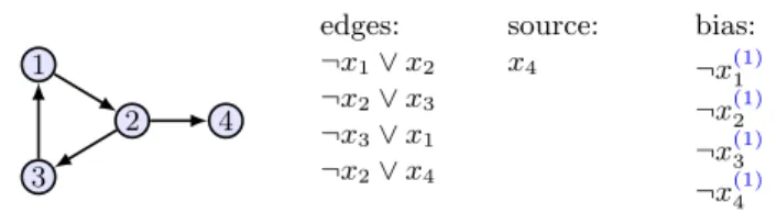
1 2 3 4 edges: ¬x1∨x2 ¬x2∨x3 ¬x3∨x1 ¬x2∨x4 source: x4 bias: ¬x(1)₁ ¬x(1)2 ¬x(1)₃ ¬x(1)₄

Fig. 1: A simple digraph and its representation as a propositional CNF formula. A clause with no weight is a hard clause; for example,x4 is the same asx(4∞). a MaxSAT solver finds a model that maximizes the sum of the weights of the satisfied clauses. Many of these concepts will be defined in the next section, in a more general setting. In this section, let us just look at an example.

Consider the graph inFigure 1. We can represent its edges by clauses which are essentially implications. Once we have these implications, we can ask which vertices are reachable from certain sources. Suppose that we choose 4 to be the source. The solver could produce the model x1 =x2 =x3 =x4 = 1, which is not what we want. We include a bias to tell the solver that variables be 0, if at all possible. The bias clauses have weight 1. None of the other clauses (encoding edges or sources) should be violated at the expense of a bias clause. Thus, we should pick their weight to be high enough. In this example, 5 would suffice. But, to avoid having to specify this high-enough weight, we allow∞as a weight. We call clauses with infinite weighthard; and we call clauses with finite weightsoft. This leads to thepartial version of weighted MaxSAT, or WPMS for short. Problem 1 (WPMS). Given a weightw and a weighted propositional CNF for-mulaφ:=V

iϕ

(wi)

i , decide ifφhas a model for which the weight of the satisfied

soft clauses is≥w.

2.2 Relational First-Order Logic with Weights

Propositional logic is too low level and too inefficient for our needs. Let us see why on the example in Figure 1. There, we have two distinct concepts: the digraph structure, and the notion of reachability. However, we could not keep these concepts apart: our choice of how to represent edges is very much driven by the goal of performing reachability queries. In this section, we will see that it is possible to keep these concepts distinct if we move to quantifier-free relational first-order logic with weights. Moreover, this representation is not only more convenient, but also enables faster solving through lazy grounding.

First-order logic has been extended with quantitative notions in many ways: possibility theory [20], Bayesian probabilities [30], Markov logic networks [19], and others. Here, we present a simple extension with weights, for which ground formulas correspond to MaxSAT instances.

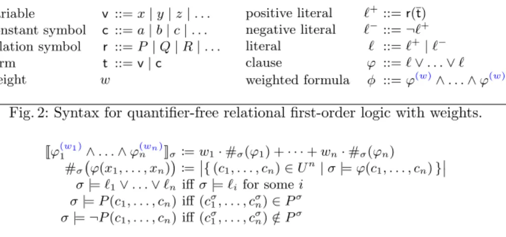
Figure 2 shows the standard syntax for quantifier-free relational first-order logic formulas in CNF, but it also introduces weights on clauses. We assume a countable set ofvariables(x, y, z, . . .), and countable sets ofsymbolsforconstants (a, b, c, . . .) andrelations(P, Q, R, . . .). Atermis a constant symbol or a variable.

variable v ::=x|y|z|. . . constant symbol c _::=a|_b|_c|_{. . .} relation symbol r _{::=P|Q|R|. . .} term t ::=v|c weight w positive literal ℓ+::=r_(¯t₎ negative literal ℓ− ::=¬ℓ+ literal ℓ ::=ℓ+|ℓ− clause ϕ ::=ℓ∨. . .∨ℓ weighted formula φ ::=ϕ(w)_{∧. . .∧ϕ}(w)

Fig. 2: Syntax for quantifier-free relational first-order logic with weights.

Jϕ(w1) 1 ∧. . .∧ϕ (wn) n Kσ :=w1·#σ(ϕ1) +· · ·+wn·#σ(ϕn) #σ ϕ(x1, . . . , xn):= {(c1, . . . , cn)∈Un|σ|=ϕ(c1, . . . , cn)}

σ|=ℓ1∨. . .∨ℓn iffσ|=ℓifor somei

σ|=P(c1, . . . , cn) iff (cσ₁, . . . , cσn)∈P σ

σ|=¬P(c1, . . . , cn) iff (cσ₁, . . . , cσn)∈/P σ

Fig. 3: Semantics for quantifier-free relational first-order logic with weights. Each relation has a fixed arity k, and takes k terms as arguments. A literal ℓ is either a relation or its negation; the former is apositive literal, the latter is a negative literal. Aclauseϕis a disjunction of literals. Aweightwis a nonnegative real number. Aweighted clause ϕ(w) _{is a clause ϕtogether with a weightw. A}

weighted formula φis a conjunction of weighted clauses. As usual, we interpret variables as universal. Occasionally, we emphasize that formulaφuses variables x1, . . . , xn by writing φ(x1, . . . , xn); similarly for clauses.

Without weights, one usually defines the semantics of formulas by specifying how they evaluate to a boolean. With weights, we define the semantics of for-mulas by specifying how they evaluate to a weight, which is a nonnegative real. In both cases, the evaluation is done on a model.

A (finite)model σ=hU,{cσ

i},{Piσ}i consists of a finiteuniverse U together

with an interpretation of (i) each constant symbolci as an elementcσi ofU, and

(ii) eachkary relation symbolPi as akary relationPiσ⊆Uk. This is a standard

setup [37, Chapter 2].

Figure 3 shows the semantics for quantifier-free relational first-order logic with weights. A clause/formula is said to be ground if it contains no variable occurrence. A ground clause ϕis said to hold in a model σwhen it contains a literal that holds in σ. A ground positive literal P(c1, . . . , cn) holds inσ when

(c1, . . . , cn) ∈ Pσ; a ground negative literal ¬P(c1, . . . , cn) holds in σ when

(c1, . . . , cn)∈/Pσ. For a clauseϕ(x1, . . . , xn) we define #σ(ϕ) to be the number

of groundings of ϕ that hold in σ. Given a model σ, the value of a weighted clause ϕ(w) _{is w·#}

σ(ϕ), and the value JφKσ of a formula φ is the sum of the

values of its clauses.

In the rest of the paper, we shall see how several practical problems concern-ing software analysis (abstraction refinement, user interaction, identifyconcern-ing likely bugs) can be phrased as instances of the following problem.

As in the case of WPMS, we allow infinite weights as a shorthand for very large weights. It is possible to show that the problem above is equivalent with exact MAP inference for Markov logic networks [19].

Example 1. Now let us revisit the example fromFigure 1. This time we represent the problem by a formulaφwith the following clauses:

edges: bias: reachability:

edge(1,2) ¬path(x, y)(1) _{path(x, x)}

edge(2,3) ¬edge(x, y)(1) _{path(x, z)∨ ¬path(x, y)∨ ¬edge(y, z)}

edge(3,1)

edge(2,4)

There are several things to note here. First, we disentangled the representation of the digraph from the queries we want to perform. The digraph structure is rep-resented by the relationedgeσ, which is specified by 5 clauses: 4 hard and 1 soft. The notion of reachability is represented by the relationpathσ, which is specified by 3 clauses: 2 hard and 1 soft. The maximum weight we can achieve isJφKσ= 15,

for example by using model σ =hU,1σ_,2σ_,3σ_,4σ_,edgeσ_,pathσ_{i with universe}

U = {1σ_,2σ_,3σ_,4σ_{}, and relationsedge ={(1}σ_,2σ_),(2σ_,3σ_),(3σ_,1σ_),(2σ_,4σ_)}

andpath= {1σ_,2σ_,3σ_{} × {1}σ_,2σ_,3σ_,4σ_}

∪ {(4σ_,4σ_)}.

We will often omit the superscript σ when there is no danger of confusing a symbol with what it denotes. Further, in all our applications we will have constant symbols to denote all elements of the universe, so we will omit listing the constant symbols explicitly. Thus, for the model in Example 1, we simply writeσ=hedge,pathi. On the topic of simplifying notation, we note that clauses are oftendefinite Horn; that is, they contain exactly one positive literal. These should be thought of as implications. So, for definite Horn clauses, we may write ℓ+1 ∧. . .∧ℓ+n (w) → ℓ+ _{instead of ℓ}− 1 ∨. . . ℓ−n ∨ℓ+ (w) .

We remark that the development so far would also work if instead of quantifier-free clauses ϕwe would have arbitrary first-order logic formulas. In particular, we could still define the notion of a weightJφKσ in the same way, and Problem2

would not change. However, we found this fragment to be expressive enough for many applications (seeSection 3), and it has the advantage that its groundings are WPMS instances. For this, we need to see ground literals as boolean variables in a WPMS instance.

Example 2. Recall Example 1. For each ground literal path(a, b) we introduce a boolean variable pab. Then, for example, the clause ¬path(x, y)(1) leads to

16 WPMS clauses, each containing one boolean variable:p(1)11, p

(1)

12, p

(1)

13, . . .

3

Applications

We demonstrate our MaxSAT based approach to tackle the central challenge of balancing different tradeoffs in software analysis. We do so by illustrating the

f() { v1 = new ...; v2 = id1(v1); v3 = id2(v2); q2: assert(v3 != v1); } id1(v) { return v; } g() { v4 = new ...; v5 = id1(v4); v6 = id2(v5); q1: assert(v6 != v1); } id2(v) { return v; } Fig. 4: Example program.

approach on three mainstream applications: automated verification (§3.1), in-teractive verification (§3.2), and static bug detection (§3.3). Specifically, we use the graph reachability analysis from Example1as an instance to explain how we can augment a conventional analysis in a systematic and general manner to bal-ance these tradoffs. Throughout, we observe a recurring theme of using weights for encoding two conceptually different quantities: costs and probabilities.

3.1 Automated Verification

A key challenge in automated verification concerns finding a program abstraction that balances efficiency and precision. A common approach to achieve such a balance is to use a strategy called CEGAR (counter-example guided abstraction refinement) [18]. To apply this strategy, however, analysis designers often resort to heuristics that are specialized to the analysis task at hand. In this section, we show how to systematically apply CEGAR to constraint-based analyses. Example. Consider the program in Figure 4. We are interested in analyzing its aliasing properties; in particular, we want to check if the two assertions at labels q1and q2 hold. Functions id1and id2 simply return their argument. It is easy to see that the assertion at q1 holds but the assertion at q2 does not. To conclude this, however, an analysis must reason precisely about the calls to functions id1 and id2. When id1 is called from f, its variable v is of course different from its variable v when called from g. Thus, the analysis should track two variants of v, one for each context. In general, however, the analysis cannot track all possible contexts, because there may be an unbounded number of them due to recursive functions. It may be prohibitively expensive to track all contexts even if there are a bounded number of them. So, for both theoretical and practical reasons, some contexts cannot be distinguished. In our example, not distinguishing the two contexts leads to considering variablevin id1 to be the same, no matter from where id1 is called. Alternatively, the calls and returns to and from id1are modelled by jumps: the return becomes a nondeterministic jump because it can go back to either f or g. This causes the analysis to conclude that the assertion at q1 might fail. Indeed, one can start the execution at the beginning off, jump intoid1when it is called, but then ‘return’ after the call to id1in g, and then continue untilq1 is reached. In summary, on the one hand, we cannot distinguish all contexts for efficiency reasons; and on the other hand, merging contexts can lead to imprecision.

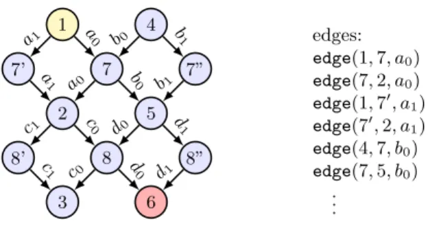
InFigure 5, we formulate an analysis that can answer whether assertions at q1andq2 hold. Our formulation is similar to the reachability problem we saw

1 7’ 2 8’ 3 7 8 4 5 6 7” 8” a 0 a0 a1 a₁ b0 b₀ b₁ b1 c₀ c0 c1 c₁ d0 d 0 d 1 d1 edges: edge(1,7, a0) edge(7,2, a0) edge(1,7′ , a1) edge(7′ ,2, a1) edge(4,7, b0) edge(7,5, b0) .. .

Fig. 5: Digraph model of the example program in Figure 4. Nodes 1, 2, and 3 stand for the basic blocks of function f; nodes 4, 5, and 6 stand for the basic blocks of functiong; nodes 7 and 8 stand for the bodies ofid1andid2, respec-tively. Nodes 7′ _{and 7}′′ _{are clones of 7; nodes 8}′ _{and 8}′′ _{are clones of 8. Edges} representing matching calls and returns have the same label.

earlier in Example1. The main difference is that edges have labels, which allows us to use them selectively.

path(x, x)

path(x, y)∧edge(y, z, u)∧abs(u)→path(x, z) (Path-Def) We have two ways to model the call from fto id1: by inlining or by a jump. Intuitively,abs(a1) means we use inlining, andabs(a0) means we use a jump.

To show that the assertion atq1holds, we need to show that there is no path from 1 to 6, forsomechoice of how to model each function call. To this end, we proceed as follows. First, we introduce the hard constraint¬path(1,6). Second, we implement a CEGAR loop. In each iteration, we have some choice of how to model each function call. We can represent this choice either by selectively generating edges, or by selectively deactivating some edges. For example, we could include all edges but deactivate some of them by including clauses

¬abs(a1) ¬abs(b1) ¬abs(c1) ¬abs(d1)

This would prevent inlining from being used. InFigure 5, we see a path from 1 to 6 that uses only edges with labels from {a0, b0, c0, d0}. This means that

¬path(1,6) is inconsistent with modelling all function calls by jumps. Thus, we should change how we model some function calls. We prefer to keep as many jumps as possible so that we do as little inlining as possible:

abs(a0)(1) abs(b0)(1) abs(c0)(1) abs(d0)(1)

The solver could answer with a model in which abs={a0, b0, c0}. In that case, in the next iteration we inline the call fromgtoid2, by including clauses

abs(a0)(1) _abs(b0)(1) _abs(c0)(1) _¬abs(d0)

Now the solution will have to disrupt the path 1 a0

→ 7 b0

→ 5 d1

→ 8′′ d1

→ 6, by not including one of a0 and b0 in abs. Suppose the solver answers withabs=

{a0, c0, d1}. Then, in the next CEGAR iteration we try to model both calls fromgby inlining.

abs(a0)(1) ¬abs(b0) abs(c0)(1) _¬abs(d0)

¬abs(a1) abs(b1) ¬abs(c1) abs(d1)

The solver returns abs = {a0, b1, c0, d1}. Since the maximum possible weight

was achieved, we know that no further refinement is needed: there exists a way to model function calls that allows us to conclude the assertion atq1holds. General Case. The core idea is to formulate the problem of finding a good ab-straction as an optimization problem on a logic with weights (see Problem2). In general, the encoding of the program need not be a digraph, and the analysis need not be reachability. However, the abstraction will often select between dif-ferent ways of modeling program semantics, and will be represented by a relation similar to the relationabsin our example. Accordingly, we model the program, the analysis, and the query by a formula φ, without relying on its structure. We define the space of abstractions to be a boolean assignment to sites. (In our example, the sites are the four function calls.) Suppose the current abstraction is A:Site_{→ {0,1}. Then, we ask for a model of maximum weight for the formula}

φ∧ ^ A(s)=0 abs(s0)(1)∧ ¬abs(s1) ∧ ^ A(s)=1 ¬abs(s0)∧abs(s1)

For eachs∈Site_{, we have two constant symbols,s0 ands1. If the formula has} a model of maximum weight, which is the number of imprecise sites, then the query is proven. If the formula has no model that satisfies all its hard clauses, then no abstraction can prove the query. Otherwise, by inspecting the model, we can find a more precise abstraction to try next.

We refer the reader to [71] for instantiations of this approach to pointer analysis and typestate analysis of Java programs.

Discussion. One can design an automated analysis that balances efficiency and precision as follows: (1) design a basic constraint-based analysis; (2) parameterize the analysis; and (3) find a good abstraction by solving an optimization problem. We saw a simple example of an analysis which tracked information flow in a program. There are, however, many other analyses that use constraint-based formulations [11,33,65–67].

What does it mean to parameterize an analysis? Compare Example1 with Figure 5. In one we have edges; in the other we have edges that can be activated or deactivated. By constraining the relationabs, we were able to model function calls either by jumps (cheap) or by inlining (expensive). The intuition is that inlining is expensive due to nesting. This intuition also holds for other context sensitivity mechanisms, such as k-CFA and k-object sensitivity. Thus, there is

1 2 3 4 5 6 7 8 a b source sink

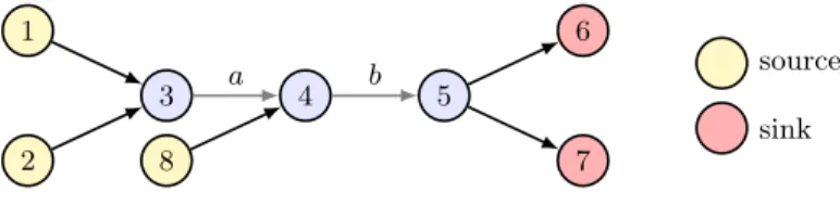
Fig. 6: First source-sink information-flow example: If some edges are spurious, then some source-sink flows are interrupted.

often a way to introduce a relation absthat tells us, for each of several sites in the program, whether to use cheap or expensive semantics.

Finally, once the relationabsis introduced, we can implement the CEGAR loop sketched above, which achieves efficiency by increasing precision selectively. In [71], multiple queries are handled simultaneously: the result of the CEGAR loop is to classify assertions into those verified and those impossible to verify. By the latter, we mean that they would not be verified by the most expensive abstraction, if we were to try it. But the CEGAR loop will typically reach the conclusion that an assertion is impossible to verify without actually trying the most expensive abstraction. Another extension [25] describes an alternate CE-GAR strategy that considers not only the relative cost of different abstractions but also their probability of success.

3.2 Interactive Verification

Sound analyses produce a large number of alarms which include a small number of real bugs. Users then sift through these alarms, classifying them into false alarms and real bugs. In other words, a computer and a user collaborate on finding bugs: in a first phase, the computer does its work; in a second phase, the user does their work. In certain situations, however, it is possible to reduce the total amount of work done by the user by interleaving: the computer and the user take turns at doing small amounts of work. The idea is that we should let users perform certain tasks they are better suited for and we should use the results of their work to guide the computer’s work.

Example. Consider the information-flow example from Figure 6. We wish to know if there are paths from sources to sinks. If the analysis runs with no help from the user, it presents the following alarms:

path(1,6) path(1,7) path(2,6) path(2,7) path(8,6) path(8,7) After inspecting all 6 alarms, the user decides that all of them are false alarms.

Now consider an alternative scenario. Suppose the analysis suspects that the edges marked asaandbmay be spurious. Then, before presenting a large set of alarms to the user, it may be beneficial to ask the user ifaorb are spurious. If ais spurious, then 4 alarms disappear; ifbis spurious, then 6 alarms disappear. It is therefore better to ask the user about edgeb. We can formulate this choice of question, betweenaandb, as an optimization problem.

As before (§3.1), we use labels on edges. The definition of reachability remains as in (Path-Def_{). But here labels represent something different: we use labels} a and b to identify each of the possibly spurious edges, and we use one extra labelc for all the other edges.

edge(3,4, a) edge(1,2, c) edge(2,3, c) edge(8,4, c)

edge(4,5, b) edge(5,6, c) edge(5,7, c) abs(c)

We require that the non-spurious edges are selected, and that at most one of the other edges are deselected:

abs(c) abs(a)∨abs(b)

Finally, we want a maximum number of alarms to disappear:

¬path(1,6)(1) _¬path(2,6)(1) _¬path(8,6)(1)

¬path(1,7)(1) _¬path(2,7)(1) _¬path(8,7)(1)

For the formula built with the clauses described so far, the model of maximum weight has abs= {a, c} and weight 6. We interpret this to mean that edge b may rule out 6 alarms.

General Case. We wish to save user time by bringing to their attention root cause of imprecision in the analysis that may be responsible for many false alarms. The core idea is to formulate the problem of finding a good question to ask the user as an optimization problem on a logic with weights (Problem2). As before (§3.1), we assume that the analysis is described by some formulaφ, and we assume the existence of a special relation abs. In addition, we also assume

that we are given a list ℓ+₁, . . . , ℓ+

n of grounded positive literals that represent

alarms. Then, we ask for a model of maximum weight for the formula φ∧ n ^ i=1 ¬ℓ+_i (1) ∧ ^ 1≤i<j≤m abs(ai)∨abs(aj) ∧abs(c)

The constants a1, . . . , am identify the possibly spurious edges, while the

con-stantc marks all the other edges. In a model of maximum weight, at most one ofa1, . . . , am will be missing from the relationabs. The missing constant

iden-tifies the question we should ask the user. The maximum weight is the number of alarms that will be classified as false, should the user answer ‘no’. If none of a1, . . . , am is missing from abs, then none of the alarms can be caused by

imprecision of the analysis.

We refer the reader to [70] for instantiations of this approach to datarace analysis and pointer analysis of Java programs.

Discussion. What if the user labels an edge as spurious when in fact it is not? In this case, real bugs may be missed, even though the original analysis is sound. One can define a notion of relative soundness to accommodate this situation:

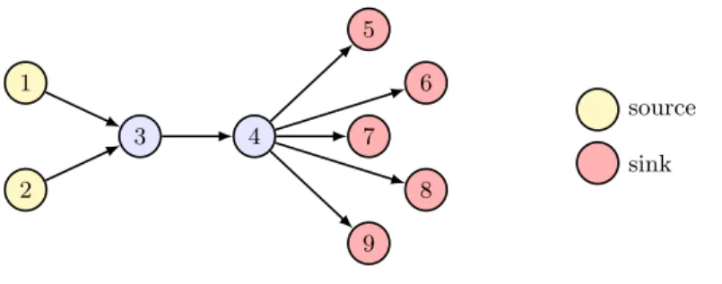
1 2 3 4 5 6 7 8 9 source sink

Fig. 7: Second source-sink information-flow example: If many flows with the same source lead to bad bug reports, then other flows from the same source arelikely to also lead to bad bug reports.

bugs are not missed as long as the user makes no mistakes in handling the analy-sis’ output. Another approach would be to check the users’ answers, which would feasible if the user not only answers ‘yes’/‘no’ but also offers extra information in the form of a certificate that supports their answer. This approach is adopted by the Ivy tool [52], which asks the user for help in finding an inductive invariant, but checks inductiveness.

Another possible concern is that the termV

1≤i<j≤mabs(ai)∨abs(aj), which

is used to ensure that we search for a single spurious edge, grows quadrati-cally. There exist efficient but non-obvious ways to encode such cardinality con-straints [22,64] and there also exist ways to handle them directly in satisfiability solvers [56]. These techniques also work for other cardinalities: we can ask what is the best set of ≤k possibly spurious edges, which may be necessary if the disappearance of any single spurious edge does not rule out any alarm. By a more involved process, it is also possible to maximize the expected number of alarms ruled outper spurious edge [70].

3.3 Static Bug Detection

In the previous section, we saw how user feedback can be used to reduce the number of false alarms produced by a sound analysis. While in theory we deal mostly with sound analyses, in practice, analysis designers must make pragmatic assumptions [38]. In this section, we assume that we start from such an analysis, which could be described as a bug finder. In this situation, we want to avoid not only false positives but also false negatives. The approach we take is to probabilistically learn from user ‘likes’ and ‘dislikes’ on bug reports. Based on this feedback, the analysis adjusts the approximations it makes.

Example. Figure 7gives an information-flow example, similar to the one in the previous section (§3.2). This time, however, edges are not labeled, so we use the simple definition of reachability from Example 1. While each edge in the graph is always valid, a path computed by the analysis can be spurious due to the approximations applied.

On this example, the analysis produces 10 reports, corresponding to the cross product of the 2 sources with the 5 sinks. There reports are mixed true alarms and false alarms. Suppose that all reports with node 2 as the source are false alarms because path(2,4) is spurious. Typically, this is where the interaction between the analysis and the user stops, and the user has to inspect each report manually. In this case, the user can quickly get frustrated due to high false positive rate (50%).

To address this challenge, we allow the analysis to incorporate user feedback and therefore produce results that are more desirable to the user. For instance, if the user inspects path(2,5) and path(2,6) and determines them to be false alarms, we incorporate this feedback and suppress path(2,7), path(2,8), and

path(2,9), which are derived for the same root cause. To achieve this effect, we need to address two challenges:

1. How can we enable a conventional analysis to incorporate user feedback in a systematic and automatic manner?

2. How can we generalize the impact of feedback on limited reports to others? For the first challenge, we notice that it is impossible to directly incorporate user feedback in a conventional analysis, which formulates the analysis problem as a decision problem. In such a decision problem, all clauses are hard, which makes the analysis rigid and define a single set of reports that cannot be changed. As a result, if we directly add the aforementioned user feedback as hard clauses

¬path(2,5) and ¬path(2,6), it will make the constraint system inconsistent. Ideally, we want the ability to occasionally ignore certain clause groundings that can introduce imprecision and therefore guide the analysis to produce results that are more desirable to the user.

Our approach addresses this challenge by attaching weights to certain clauses whose groundings can introduce false alarms and therefore convert them from hard into soft. Intuitively, the weight of a clause represents the analysis writer’s confidence in it: the higher weight it has, the less likely the writer thinks it will introduce imprecision. These weights can be specified by the analysis writer manually or automatically learnt from training programs whose bug reports are fully labeled using standard algorithms [62]. The clauses that are considered precise remain as hard clauses.

The above transformation results in a probabilistic analysis specified in logic with weights, which defines a distribution of outputs rather than a single output. We call this analysis probabilistic as the clause groundings now hold with some probability. And the final set of bug reports is the most likely one that maximizes the sum of the weights of the satisfied clause groundings. Moreover, it allows us to incorporate user feedback as new clauses in the system, which will change the output distribution and the set of bug reports. Since the user can make mistakes, we also add user feedback as soft clauses to the system, whose weights represent the user’s confidence in them and can be also trained from labeled data. Intuitively, the bug reports produced after feedback are the ones that the analysis writer and the analysis user will most likely agree upon.

For the example analysis, we observe that reflexivity ofpath always holds,

while transitivity of path can introduce imprecision. As a result we attach a weight to the clause which encodes transitivity, say 100. We also add user feed-back as clauses ¬path(2,5)(200) _{and ¬path(2,6)}(200)_{. We attach high weights}

to user feedback clauses as we assume the user is confident in the feedback. As a result, we obtain the analysis specification with user feedback in logic with weights below:

Rules: Bias: Feedback:

path(x, x) ¬edge(x, y)(1) _¬path(2,5)(200)

path(x, y)∧edge(y, z)(100)−→path(x, z) ¬path(x, y)(1) _¬path(2,6)(200)

We now discuss how our approach addresses the second challenge, of gener-alizing user feedback from some reports to others. We observe that all five false alarms are derived due to the spurious fact path(2,4), which reveals a more general insight about false alarms: most false alarms are symptoms of a few root causes. Rectifying these few root causes (path(2,4) in the example) can signif-icantly improve the analysis precision. We illustrate how our approach achieves this effect by studying the MaxSAT instance generated by the above analysis specification with feedback:

c1: path(2,2) ∧

c2: path(2,3)∨ ¬path(2,2)∨ ¬edge(2,3)(100) _∧

c3: path(2,4)∨ ¬path(2,3)∨ ¬edge(2,4)(100) _∧

c4: path(2,5)∨ ¬path(2,4)∨ ¬edge(4,5)(100) _∧

c5: path(2,6)∨ ¬path(2,4)∨ ¬edge(4,6)(100) ∧ c6: path(2,7)∨ ¬path(2,4)∨ ¬edge(4,7)(100) _∧

c7: path(2,8)∨ ¬path(2,4)∨ ¬edge(4,8)(100) _∧

c8: path(2,9)∨ ¬path(2,4)∨ ¬edge(4,9)(100) ∧

f1:¬path(2,5)(200) _∧

f2:¬path(2,6)(200) _∧

...

For the purpose of illustration, we only show the clauses that are related to the false alarms. In addition, we elide the bias clauses and assume that the computed model is always minimal. We notice that clauses c1-c5 form a con-flict with the feedback clauses f1 and f2. As a result, a model of the MaxSAT instance cannot satisfy all of them. To maximize the sum of the weights of sat-isfied soft clauses, the model will violatec3 while satisfying the other aforemen-tioned clauses. Hence, variables path(2,4), path(2,5), path(2,6) will be set to falsein the solution. Since the computed model is minimal, variablespath(2,7),

path(2,8), path(2,9) will also be set to false, which correspond to the other

false alarms that are derived frompath(2,4). Hence, we successfully generalize the impact of the feedback on reports path(2,5) and path(2,6) by eliminating their common root cause path(2,4), which in turn suppresses the other three false alarms that are derived from it.

General Case. We now discuss the general recipe for our approach. It is divided into an offline learning phase and an online inference phase. The offline phase takes a conventional analysis specified by an analysis writer and produces a prob-abilistic analysis specified in logic with weights. It produces the weight for each clause by learning it from training programs whose bug reports are fully labeled. The online phase applies the probabilistic analysis on a program supplied by the analysis user and produces bug reports in an interactive way. In each iteration, the user selects and inspects a subset of reports produced by the analysis, and provides positive or negative feedback. The analysis incorporates the feedback and update the reports for the next iteration. This interaction continues until all the bug reports are resolved.

We refer the reader to [40] for instantiations of this approach to datarace analysis and monomorphic call site analysis of Java programs.

Discussion. This approach is similar to the one introduced in§3.2as they both improve the analysis accuracy by incorporating user effort. However, while the previous approach requires the user to inspect intermediate analysis facts, the current approach directly learns from user feedback on end reports. As a result, the previous approach requires the user to understand intermediate analysis results but the current approach does not. On the other hand, the previous approach can guarantee the soundness of the result if the user always gives correct answers, while the current approach may introduce false negatives due to its probabilistic nature. Hence, the current approach is more suitable for bug finding whereas the previous approach can be applied in interactive verification.

4

Techniques

We present techniques we have developed for MaxSAT solving. While primarily motivated by the domain of software analysis, they are general enough to be applicable to other domains too such as Big Data analytics and statistical AI.

We present a framework embodying our general approach (§4.1). We then present two techniques as instantiations of the framework (§4.2). We also present two techniques that enable to optimize the framework (§4.3).

4.1 Framework

Our framework targets the problem of finding a model of a relational first-order logic formula with weights. The standard approach consists of two phases: grounding and solving. In the grounding phase, the formula is reduced to a WPMS instance by instantiating all variables with all possible constants. In the solving phase, the WPMS instance is solved using an off-the-shelf WPMS solver. Both phases are challenging to scale: in the grounding phase, naively instanti-ating all variables with all possible constants can lead to an intractable WPMS instance (comprising upto 1030 _{clauses); in the solving phase, the WPMS} prob-lem itself is also a combinatorial optimization probprob-lem, known for its intractabil-ity [4,42]. We address both these challenges by interleaving the two phases in an

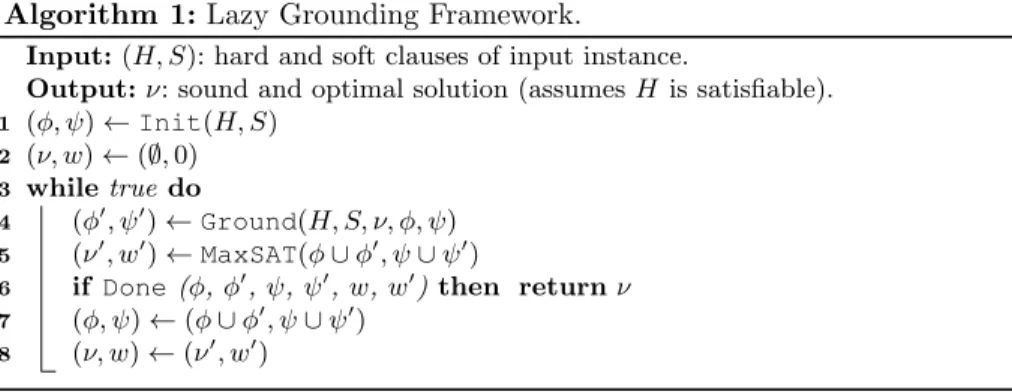
Algorithm 1: Lazy Grounding Framework.

Input:(H, S): hard and soft clauses of input instance.

Output:ν: sound and optimal solution (assumesH is satisfiable). 1 (φ, ψ)←Init(H, S) 2 (ν, w)←(∅,0) 3 whiletruedo 4 (φ′, ψ′)←Ground(H, S, ν, φ, ψ) 5 (ν′, w′)←MaxSAT(φ∪φ′, ψ∪ψ′) 6 _if Done(φ,φ′ ,ψ,ψ′ ,w, w′ )then returnν 7 (φ, ψ)←(φ∪φ′, ψ∪ψ′) 8 (ν, w)←(ν′, w′)

iterative lazy grounding process that progressively expands a subset of clauses while providing soundness and optimality guarantees.

Grounder MaxSAT Solver new clauses ("’,%&’) initial clauses (",%&) Checker candidate

solution (’ sound and optimal solution ( Yes No Initializer input instance (H,%S)

Fig. 8: Architecture of our lazy grounding framework for solving large MaxSAT instances. It scales by iteratively expanding a workset comprising a subset of clauses in the input MaxSAT instance. Our bottom-up and top-down grounding techniques, and many others in the literature, are instances of this framework.

The architecture of our framework is depicted in Figure 8 and its overall algorithm is presented as Algorithm1. For elaboration, we divide a weighted logic formula into separate hard clauses (denoted byH) and soft clauses (denoted by S). The framework is parametric in three procedures:Init,Ground, andDone. It begins by invoking the Init procedure on line 1 to compute an initial set of hard clausesφand soft clausesψ. Next, it executes the loop defined on lines 3–8. In each iteration of the loop, the algorithm keeps track of a pair comprising the new solutionν′_{and its weightw}′_{, which is the sum of the weights of the soft} clauses satisfied byν′_{. On line4, it invokes theGroundprocedure to compute} the set of hard clausesφ′ _{and soft clausesψ}′_{to ground next. Typically,φ}′_andψ′ correspond to the set of hard and soft clauses violated by the previous solution ν. On line5, the current hard and soft clauses and the newly grounded hard and soft clauses are fed to an off-the-shelf WPMS solver to produce a new solution ν′ _{and its corresponding weight w}′_{. Initially, the solution is empty with weight} zero (line2). Next, on line6, the algorithm checks ifν satisfies the terminating

Algorithm 2: Bottom-Up Approach 1 _Procedure Init(H,S) 2 (φ, ψ)←(∅,∅) 3 _return(φ,ψ) 4 _Procedure Ground(H,S,ν,φ,ψ) 5 (φ, ψ)←(∅,∅) 6 _foreachh∈H _do 7 if ν2JhKσ then φ←φ∪JhKσ 8 _foreach(w, h)∈S _do 9 _if ν2JhK_{σ then} ψ←ψ∪ {(w, ρ)|ρ∈JhK_σ} 10 return(φ,ψ) 11 Procedure Done(φ, φ’,ψ,ψ’, w, w’) 12 _return φ′=∅ ∧w=w′

condition by invoking the Done procedure. If not, then on line 7, both sets of grounded clausesφ′ _andψ′_{are added to the corresponding sets of grounded hard} clauses φand grounded soft clausesψ respectively. Accordingly, the solution ν and its corresponding weightw are updated as well.

Different instantiations of the three procedures that parameterize our frame-work yield different grounding algorithms proposed in the literature [14,35,39, 41,50,51,54]. We broadly classify instantiations of the framework into two cat-egories akin to top-down and bottom-up approaches to Datalog evaluation [2]. We next present one instantiation that we have developed in each category.

4.2 Instantiations

Applications built upon constraint-based approaches are typically only con-cerned with the assignment to certain variables of interest, which we refer to as queries. The bottom-up approach computes an assignment to all variables from which one can subsequently extract the assignment to queries. The top-down approach, on the other hand, only grounds clauses that are needed to compute the assignment to queries. This approach offers significant performance gains when queries comprise a small fraction of all variables, which is the case in many applications. We introduced the top-down approach for MaxSAT in [72]. Bottom-Up Approach. Algorithm 2 presents our bottom-up instantiation from [39]. Procedure Init returns an empty set of hard ground clauses and an empty set of soft ground clauses (line 2). For each hard clause in the input instance, procedure Ground checks if the current solution violates any of its groundings and includes those violated ground clauses as new hard clauses (lines 6-7). Similarly, Ground also includes violated soft ground clauses (lines 8-9), and they share the same weight as the corresponding soft clause in the input instance. Given hard and soft ground clauses and the corresponding solu-tions from two successive iterasolu-tions, procedureDonechecks whether the current

Algorithm 3: Top-Down Approach 1 _Procedure Init(H,S)

2 (φ, ψ)←(∅,∅)

3 _foreach(w, h)∈S _do 4 foreachρ∈JhKσ do

5 _if any variable ofρ∈ Q_then ψ←ψ∪ {(w, ρ)} 6 initializeφin a similar way without considering weights 7 _return(φ,ψ) 8 Procedure Ground(H,S,ν,φ,ψ) 9 (φ′, ψ′)←(∅,∅) 10 V ←variables used inφ∪ψ 11 _foreach(w, h)∈S _do 12 _foreachρ∈JhK_{σ do}

13 if (w, ρ)∈/ψ ∧ ν2ρ ∧any variable ofρ∈V then 14 ψ′←ψ′∪ {(w, ρ)}

15 updateφ′ in a similar way without considering weights 16 w←evaluate(ψ, ν) 17 (ν′, w′)←MaxSAT(φ∪φ′, ψ∪ψ′) 18 _if φ′=∅ ∧w=w′ _then 19 return (∅,∅) 20 else 21 ψ′_s← {(w, ρ)∈ψ′|ν′|=ρ} 22 return(φ′, ψ′_s) 23 _Procedure Done(φ, φ’,ψ,ψ’, w, w’) 24 _return φ′=∅ ∧ψ′=∅

solution is a sound and optimal solution. Specifically, Done returns true if no hard clauses in the input instance are violated (i.e.,φ′_{=∅) and the weight of the} current solution equals the weight of the last solution (i.e.,w=w′_{). Intuitively,} it means that we cannot improve the solution further even we consider more ground clauses.

SoftCegar [14] and Cutting Plane Inference (CPI) [51,54] are instances of the bottom-up approach. SoftCegar uses a slight variant that grounds all the soft clauses upfront but lazily grounds the hard clauses, while CPI employs a more conservative instantiation of Done.

Top-Down Approach. A top-down approach aims to find a partial assignment to queries such that there exists a completion of it that is a sound and optimum solution to the full problem. Algorithm3shows a naive top-down instantiation. More advanced instantiations are presented in [72]. TheInitprocedure returns all soft and hard ground clauses that involve at least one of the queried variables (denoted byQ) (lines3–6). For ease of exposition, the pseudo code of theInit procedure explicitly enumerates all ground clauses. In practice, it is implemented

Algorithm 4: Optimization with eager proofs 1 _Procedure Init(H,S) 2 (φ, ψ)←(∅,∅) 3 φ′←initial facts 4 while φ′*φdo 5 φ←φ∪φ′ 6 foreachh∈H do 7 _foreachρ∈JhKσ do 8 _if ρ=Vn i=1ti =⇒ t0 then 9 if Vn i=1ti∈φthen 10 φ′←φ′∪ {t₀} 11 _return(φ,ψ) 12 Procedure Done(φ, φ’,ψ,ψ’, w, w’) 13 _return φ′=∅ ∧w=w′

using symbolic approaches such as SQL queries [50] for efficiency. TheGround procedure returns ground clauses that may help improve the current solution. To achieve this goal, it first searches for ground clauses (φ′_{, ψ}′_{) that 1) are} not in the work set, but 2) share variables with clauses int it, and 3) are not satisfied by the current solutionν (line 9-15). Then it checks whether the current solutionν violates any ground hard clauses inφ′ _{and whether the weight of the} solution can be improved by considering (φ′_{, ψ}′_{) (line 16-22). It checks the latter} condition by computing the solution (denoted byν′_{) to (φ∪φ}′_{, ψ∪ψ}′_{) and the} corresponding weight (denoted by w′_{) (line 16-17). If neither condition holds,} it returns empty sets of ground clauses and concludes that the current solution cannot be improved further. Otherwise, it returns the hard ground clauses inφ′ that are violated byν and the soft ground clauses inψ′ _{that are satisfied byν}′ as these ground clauses will highly likely improve the current solution. It follows that the top-down approach terminates whenGroundreturns empty sets. The correctness of Algorithm3is proved in [72].

4.3 Optimizations

We introduce two optimizations to further improve the efficiency of our frame-work: eager grounding and incremental solving.

Eager Grounding. Our first observation is that most constraints in domains like software analysis are Horn clauses. Horn clauses form a set of proof-tree like structures. When one of them is violated by the solution of the current iteration in lazy grounding, many others will be violated in the next iteration, which in turn will cause a chain effect in the subsequent iterations. We can avoid such chain effects by eager proof exploitation [39], which computes an optimal initial grounding for Horn clauses. TheInitprocedure of Algorithm4

Algorithm 5: Fu & MalikAlgorithm with partial weights [4,42] Input:φ=φH∪φS

Output:optimal solution toφ

1 whiletruedo

2 (st, ν, φC)←SAT(φ,A)

3 if st=SATthen returnν // optimal solution to φ

4 VR← ∅ // relax variables of the core

5 w_min←min{w|c∈φ_C∧(w, c)∈φ_S} 6 _foreachc∈φC do

7 _if (w, c)∈φ_{S then}

8 VR←VR∪ {r} // r is a fresh relaxation variable 9 φ←φ\ {(w, c)} ∪ {(w−wmin, c),(wmin, c∨r)} // split soft

clauses

10 if VR=∅then returnunsat // no soft clauses in the core 11 φ←φ∪CN F(P

r∈VRr≤1) // add hard cardinality constraint

shows the optimization with eager proofs, which starts with initial facts as hard clauses and iteratively applies Horn clauses to derive new facts as hard clauses. Theorem 1 shows the optimality of the Init procedure. Though Theorem 1 gives no guarantee of the necessity to ground soft Horn clauses upfront, we find that it is also helpful in practice. The eager proof exploitation procedure can be efficiently implemented using an off-the-shelf Datalog engine.

Theorem 1. (Optimal initial grounding for Horn clauses)Initin Algo-rithm4grounds all necessary hard Horn clauses and no more hard Horn clauses need to be grounded in later phases.

Proof. See the proof in Appendix A of [39]. ⊓⊔

Incremental Solving. Our framework generates a sequence of MaxSAT in-stances, and the MaxSAT instance in the next iteration is generated by append-ing new hard or soft clauses to the MaxSAT instance in the current iteration. Formally, we have asequential MaxSAT problem: (φ1_{, ψ}1_),(φ2_{, ψ}2_{), ...,(φ}n_{, ψ}n_),

withφk _⊆φk+1_{, ψ}k_⊆ψk+1_{. A straightforward solution is toindependentlysolve} each MaxSAT instance (φk_{, ψ}k_{) using an off-the-shelf MaxSAT solver. This is}

the approach used by most applications [17,39,40,71]. Next we show that by leveraging the sequential property,incremental core-guidedMaxSAT solving [61] can solve the sequential MaxSAT problem more efficiently.

The unsat core-guided MaxSAT algorithm, also known asFu & Malik algo-rithm [24], forms the basis of many popular MaxSAT algoalgo-rithms [4,42,44,47]. Algorithm5shows theFu & Malikalgorithm extended with partial weights. The algorithm iteratively calls a SAT solver and relaxes unsatisfiable subformula. Ini-tially,φconsists of all hard and soft constraints from inputs. In each iteration, it calls SAT solver onφ, which returns a triple (st, ν, φC). Ifstis satisfiable,νis the

optimal solution; otherwise, φC will be an unsatisfiable subformula (or UNSAT

core) of φ. Then, it computes the minimum weightwmin of soft constraints in

the UNSAT core (line-5). For each soft constraint in the UNSAT core, it splits the soft constraint into two soft constraints: one with the same constraint but with weight reduced bywmin, the other one with original constraint relaxed by

a newly created variable and with weight wmin (lines6-9). If there are no soft

constraints in the UNSAT core, it returns UNSAT as there exists a conflict in hard constraints (line-10). Otherwise, a new hard constraint is added toφsuch that at most one of soft constraints in UNSAT core can be relaxed (line-11).

There are two levels of incrementality we can explore to improve Algorithm5. Similar to sequential MaxSAT problem, solving an individual MaxSAT instance involves a sequence of SAT problems. So, the first level of incrementality is to use SAT solver in an incremental way. Martins et al. [44] propose incremental blocking technique to leverage incremental SAT solving [21]. We propose the second level of incrementality, which is across of MaxSAT instances. The key idea is to reuse UNSAT cores, which can be achieved by slightly revising Algorithm5. When thek-th MaxSAT instance is solved1_{at line-5, instead of returning solution} and exiting, we can output the current solution fork-th instance, then read the newly added constraints (φk+1_\φk_{, ψ}k+1_\ψk_{) for (k+1)-th instance and jump to}

line-3. This approach is correct because the addition of new soft or hard clauses does not invalidate any of the previously found UNSAT cores.

An interesting observation we have is that the incremental solving does not always improve performance; on the contrary, it may even deteriorate perfor-mance. Our experience indicates that UNSAT cores with low weight discovered in earlier instances could cause too many splittings, especially when soft con-straints with high weights are added later. To resolve this issue, we propose a restart mechanism, which restarts the current MaxSAT instance solving after detecting any low quality cores. We empirically find that the number of split-tings of each individual soft constraint is an effective quality measurement, and that restarting after the maximum number of splitting is more than 5 achieves best performance on our applications.

5

Related Work

We survey work on MaxSAT applications and techniques for MaxSAT solving. Applications. MaxSAT has been widely used in many domains [6,13,15,23, 26,31,32,34,57,68,69,73]. The Linux package manage tool OPIUM [68] uses MaxSAT to find the optimal package install/uninstall configuration. Walter et al. [69] apply MaxSAT in industry automotive configurations. Zhu et al. [73] apply MaxSAT to localize faults in integrated circuits. By combining bounded model checking and MaxSAT, BugAssist [32] performs error localization for C

1 _{We assume hard constraints can be satisfied; otherwise hard constraints of all future}

programs, and ConcBugAssist [34] finds concurrency bugs and recommends re-pairs. Jin et al. [31] show how to improve the performance and accuracy of error localization using MaxSAT. To detect malware in Android apps, ASTROID [23] automatically learns semantic malware signatures by using MaxSAT to find the maximally suspicious common subgraph from a few samples of a malware family. Besides, MaxSAT is also helpful in visualization [13], industrial designs [15,57], reasoning about biological networks [26], and various data analysis tasks [6]. Techniques. There are a number of different approaches for exact MaxSAT solving, including branch-and-bound based, satisfiability-based, unsatisfiability-based, and their combinations [5,8,27,29,43,44,46–48]. The most successful of these on real-world instances, as witnessed in annual MaxSAT evaluations [1], perform iterative solving using a SAT solver as an oracle in each iteration [5,47]. Such solvers differ primarily in how they estimate the optimal cost (e.g., linear or binary search), and the kind of information that they use to estimate the cost (e.g. cores, the structure of cores, or satisfying assignments). Many algorithms have been proposed that perform search on either upper bound or lower bound of the optimal cost [5,46–48], Some algorithms efficiently perform a combined search over both bounds [27,29]. A drawback of the most sophisticated com-bined search algorithms is that they modify the formula using expensive Pseudo Boolean (PB) constraints that increase the size of the formula and potentially hurt the solver’s performance. A recent approach [8] avoids this problem by us-ing succinct formula transformations that do not use PB constraints and can be applied incrementally. Lastly, similar to our optimizations in§4.3, many other techniques (e.g., [7,28]) also focus on optimizing Horn clauses.

6

Future Directions

We plan to extend our approach in three directions to further advance constraint-based analysis using MaxSAT: constraint languages, solver techniques, and ex-plainability of solutions.

Language Features. As discussed in Section 2, since propositional formulae are too low-level for effectively specifying software analyses, we use relational first-order logic with weights as our constraint language. While it suffices for applications and analyses described in our previous work [25,40,70,71], it can be further improved with richer features, two of which we discuss below.

While the current logic excels at specifying analysis problems that can be succinctly expressed in relational domains, it has difficulties in expressing analy-sis problems in integer, real, string, and other domains. Akin to how Satisfiability Modulo Theories (SMT) extends SAT, we can handle these domains by incorpo-rating their corresponding theories in our language via techniques similar to the Nelson-Oppen approach. One emerging language for such problem is Maximum Satisfiability Modulo Theories (MaxSMT) [9,10,16,36,49,59,60].

The other feature is the support for the least fixpoint operator, as almost all software analyses involve computing the least fixpoint of certain equations.

Our current constraint language supports this operator indirectly by requiring additional soft clauses to bias the solution to a minimal model. However, a built-in least fixpobuilt-int operator would be much more preferred. First, it elimbuilt-inates the need for the aforementioned soft constraints which can complicate the process of analysis design as they may interact with other soft constraints. Secondly, by including the operator explicitly in the language, the underlying solver can exploit more efficient algorithms that are specialized for handling least fixpoints. Solver Techniques. We describe four techniques that can further improve the effectiveness of our solving framework.

Magic Sets Transformation. Akin to their counterparts in Datalog evalu-ation, the top-down approaches and the bottom-up approaches have different advantages and disadvantages. One promising idea to combine their benefits without their drawbacks is Magic Set transformation [55]. The idea is to apply the bottom-up approaches but rewrite the constraint formulation so that the constraint solving is driven by the demand of queries. In this way, we are able to only consider the clauses that are related to the queries while leveraging efficient solvers of the bottom-up approaches.

Lifted Inference. While our current grounding-based framework effectively leverages advances in MaxSAT solvers, it loses the high-level information while translating problems in our constraint language into low-level propositional for-mulae. Lifted inference [12,45,53,58,63] is a technique that aims to solve the constraint problem symbolically without grounding. While lifted inference can effectively avoid grounding large propositional formulae for certain problems, it fails to leverage existing efficient propositional solvers. One promising direction is to combine lifted inference with our grounding approach in a systematic way. Compositional Solving. By exploiting modularity of programs, we envision compositional solving as an effective approach to improve the solver efficiency. The idea is to break a constraint problem into more tractable subproblems and solve them independently. It is motivated by the success of compositional and summary-based analysis techniques in scaling to large programs.

Approximate Solving.Despite all the domain insights we exploit, MaxSAT is a combinatorial optimization problem, which is known for its intractability. As a result, there will be pathological cases where none of the aforementioend tech-niques are effective. One idea to address this challenge is to investigate approx-imate solving, which trades precision for efficiency. Moreover, to trade precision for efficiency is a controlled manner, it is desirable to design an algorithm with tunable precision.

Explainability. Software analyses often return explanations along with the results, which are invaluable to their usability. For example, a typical bug find-ing tool not only returns the software defects it finds but also inputs that can trigger these defects. However, in the case of constraint-based analysis, the un-derlying constraint solver must provide explanations of the solutions to enable such functionality. While SAT and SMT solvers provide such information in the form of resolution graphs (in the case of satisfiable results) and UNSAT cores (in

the case of unsatisfiable results), how to provide explanations for optimization solvers remains an open problem.

7

Conclusion

We proposed a MaxSAT based approach to tackle the central challenge of bal-ancing different tradeoffs in software analysis. We demonstrated the approach on mainstream applications concerning automated verification, interactive veri-fication, and static bug detection. The MaxSAT instances posed in these appli-cations transcend the reach of existing MaxSAT solvers in terms of scalability, soundness, and optimality. We presented a lazy grounding framework to solve such instances. We proposed new grounding techniques as instantiations of this framework as well as optimizations to the framework.

Acknowledgments. This work was supported by DARPA under agreement #FA8750-15-2-0009, NSF awards #1253867 and #1526270, and a Facebook Fel-lowship. The U.S. Government is authorized to reproduce and distribute reprints for Governmental purposes notwithstanding any copyright thereon.

References

1. MaxSAT evaluations. http://www.maxsat.udl.cat/

2. Abiteboul, S., Hull, R., Vianu, V.: Foundations of databases: the logical level. Addison-Wesley Longman Publishing Co., Inc. (1995)

3. Aiken, A.: Introduction to set constraint-based program analysis. Sci. Comput. Program. (1999)

4. Ans´otegui, C., Bonet, M.L., Levy, J.: Solving (weighted) partial MaxSAT through satisfiability testing. In: SAT (2009)

5. Ans´oTegui, C., Bonet, M.L., Levy, J.: SAT-based MaxSAT algorithms. Artificial Intelligence 196, 77–105 (Mar 2013)

6. Berg, J., Hyttinen, A., J¨arvisalo, M.: Applications of MaxSAT in data analysis. In: Pragmatics of SAT (2015)

7. Bjørner, N., Gurfinkel, A., McMillan, K., Rybalchenko, A.: Horn Clause Solvers for Program Verification, pp. 24–51. Springer International Publishing, Cham (2015),

http://dx.doi.org/10.1007/978-3-319-23534-9_2

8. Bjorner, N., Narodytska, N.: Maximum satisfiability using cores and correction sets. In: IJCAI (2015)

9. Bjørner, N., Phan, A.D.: νZ: Maximal satisfaction with Z3. In: Proceedings of International Symposium on Symbolic Computation in Software Science (SCSS) (2014)

10. Bjørner, N., Phan, A.D., Fleckenstein, L.: νZ - an optimizing SMT solver. In: TACAS (2015)

11. Bravenboer, M., Smaragdakis, Y.: Strictly declarative specification of sophisticated points-to analyses. In: OOPSLA (2009)

12. den Broeck, G.V., Taghipour, N., Meert, W., Davis, J., Raedt, L.D.: Lifted prob-abilistic inference by first-order knowledge compilation. In: IJCAI (2011)

13. Bunte, K., J¨arvisalo, M., Berg, J., Myllym¨aki, P., Peltonen, J., Kaski, S.: Optimal neighborhood preserving visualization by maximum satisfiability. In: AAAI (2014) 14. Chaganty, A., Lal, A., Nori, A., Rajamani, S.: Combining relational learning with

SMT solvers using CEGAR. In: CAV (2013)

15. Chen, Y., Safarpour, S., Marques-Silva, J., Veneris, A.: Automated design debug-ging with maximum satisfiability. IEEE Transactions on Computer-Aided Design of Integrated Circuits and Systems 29(11), 1804–1817 (Nov 2010)

16. Cimatti, A., Franz´en, A., Griggio, A., Sebastiani, R., Stenico, C.: Satisfiability modulo the theory of costs: Foundations and applications. In: TACAS (2010) 17. Cimatti, A., Griggio, A., Schaafsma, B.J., Sebastiani, R.: A modular approach to

MaxSAT modulo theories. In: SAT (2013)

18. Clarke, E.M., Grumberg, O., Jha, S., Lu, Y., Veith, H.: Counterexample-guided abstraction refinement. In: Computer Aided Verification, 12th International Con-ference, CAV 2000, Chicago, IL, USA, July 15-19, 2000, Proceedings. pp. 154–169 (2000)

19. Domingos, P., Lowd, D.: Markov Logic: An Interface Layer for Artificial Intelli-gence. Synthesis Lectures on Artificial Intelligence and Machine Learning, Morgan & Claypool Publishers (2009)

20. Dubois, D., Prade, H.: Computational Logic, Handbook of the History of Logic, vol. 7, chap. Possibilistic Logic – An Overview. Newnes (2014)

21. E´en, N., S¨orensson, N.: Temporal induction by incremental SAT solving. Electronic Notes in Theoretical Computer Science 89(4), 543 – 560 (2003), http://www. sciencedirect.com/science/article/pii/S1571066105825423

22. E´en, N., S¨orensson, N.: Translating pseudo-boolean constraints into SAT. JSAT (2006)

23. Feng, Y., Bastani, O., Martins, R., Dillig, I., Anand, S.: Automated synthesis of semantic malware signatures using maximum satisfiability. In: NDSS (2017) 24. Fu, Z., Malik, S.: On solving the partial MAX-SAT problem. In: SAT (2006) 25. Grigore, R., Yang, H.: Abstraction refinement guided by a learnt probabilistic

model. In: POPL (2016)

26. Guerra, J.a., Lynce, I.: Reasoning over biological networks using maximum satis-fiability. In: CP (2012)

27. Heras, F., Morgado, A., Marques-Silva, J.: Core-guided binary search algorithms for maximum satisfiability. In: AAAI (2011)

28. Hojjat, H., Rmmer, P., McClurg, J., ern, P., Foster, N.: Optimizing Horn solvers for network repair. In: FMCAD (2016)

29. Ignatiev, A., Morgado, A., Manquinho, V., Lynce, I., Marques-Silva, J.: Progression in maximum satisfiability. In: ECAI (2014)

30. Jensen, F.V., Nielsen, T.D.: Bayesian Networks and Decision Graphs. Springer (2007)

31. Jin, W., Orso, A.: Improving efficiency and accuracy of formula-based debugging. In: HVC (2016)

32. Jose, M., Majumdar, R.: Cause clue clauses: Error localization using maximum satisfiability. In: PLDI (2011)

33. Kastrinis, G., Smaragdakis, Y.: Hybrid context sensitivity for points-to analysis. In: PLDI (2013)

34. Khoshnood, S., Kusano, M., Wang, C.: Concbugassist: Constraint solving for di-agnosis and repair of concurrency bugs. In: ISSTA (2015)

35. Kok, S., Sumner, M., Richardson, M., Singla, P., Poon, H., Lowd, D., Domingos, P.: The Alchemy system for statistical relational AI. Tech. rep., Department of

Computer Science and Engineering, University of Washington, Seattle, WA (2007),

http://alchemy.cs.washington.edu

36. Li, Y., Albarghouthi, A., Kincaid, Z., Gurfinkel, A., Chechik, M.: Symbolic opti-mization with SMT solvers. In: POPL (2014)

37. Libkin, L.: Elements of Finite Model Theory. Springer (2004)

38. Livshits, B., Sridharan, M., Smaragdakis, Y., Lhot´ak, O., Amaral, J.N., Chang, B.E., Guyer, S.Z., Khedker, U.P., Møller, A., Vardoulakis, D.: In defense of soundi-ness: a manifesto. CACM (2015)

39. Mangal, R., Zhang, X., Kamath, A., Nori, A.V., Naik, M.: Scaling relational infer-ence using proofs and refutations. In: AAAI (2016)

40. Mangal, R., Zhang, X., Nori, A.V., Naik, M.: A user-guided approach to program analysis. In: FSE (2015)

41. Mangal, R., Zhang, X., Nori, A.V., Naik, M.: Volt: A lazy grounding framework for solving very large MaxSAT instances. In: SAT (2015)

42. Manquinho, V.M., Marques-Silva, J.P., Planes, J.: Algorithms for weighted boolean optimization. In: SAT (2009)

43. Marques-Silva, J., Planes, J.: Algorithms for maximum satisfiability using unsat-isfiable cores. In: DATE (2008)

44. Martins, R., Joshi, S., Manquinho, V., Lynce, I.: Incremental cardinality con-straints for MaxSAT. In: CP (2014)

45. Milch, B., Zettlemoyer, L.S., Kersting, K., Haimes, M., Kaelbling, L.P.: Lifted probabilistic inference with counting formulas. In: AAAI (2008)

46. Morgado, A., Dodaro, C., Marques-Silva, J.: Core-guided MaxSAT with soft car-dinality constraints. In: CP (2014)

47. Morgado, A., Heras, F., Liffiton, M., Planes, J., Marques-Silva, J.: Iterative and core-guided MaxSAT solving: A survey and assessment. Constraints 18(4), 478–534 (Oct 2013),http://dx.doi.org/10.1007/s10601-013-9146-2

48. Narodytska, N., Bacchus, F.: Maximum satisfiability using core-guided MaxSAT resolution. In: AAAI (2014)

49. Nieuwenhuis, R., Oliveras, A.: On SAT Modulo Theories and Optimization Prob-lems (2006)

50. Niu, F., R´e, C., Doan, A., Shavlik, J.W.: Tuffy: Scaling up statistical inference in markov logic networks using an RDBMS. In: VLDB (2011)

51. Noessner, J., Niepert, M., Stuckenschmidt, H.: RockIt: Exploiting parallelism and symmetry for MAP inference in statistical relational models. In: AAAI (2013) 52. Padon, O., McMillan, K.L., Panda, A., Sagiv, M., Shoham, S.: Ivy: safety

verifica-tion by interactive generalizaverifica-tion. In: PLDI (2016)

53. Poole, D.: First-order probabilistic inference. In: IJCAI (2003)

54. Riedel, S.: Improving the accuracy and efficiency of MAP inference for Markov Logic. In: UAI (2008)

55. Ross, K.A.: Modular stratification and magic sets for DATALOG programs with negation. In: PODS (1990)

56. Roussel, O., Manquinho, V.M.: Pseudo-boolean and cardinality constraints. In: Handbook of Satisfiability. IOS Press (2009)

57. Safarpour, S., Mangassarian, H., Veneris, A., Liffiton, M.H., Sakallah, K.A.: Im-proved design debugging using maximum satisfiability. In: FMCAD (2007) 58. de Salvo Braz, R., Amir, E., Roth, D.: Lifted first-order probabilistic inference. In:

IJCAI (2005)

59. Sebastiani, R., Tomasi, S.: Optimization in SMT withLA(Q) cost functions. In: IJCAR (2012)